
Simulation of Depth of Wear of Eco-Friendly Concrete Using Machine Learning Based Computational Approaches

 ,
,  , , , ,
Abstract
:1. Introduction
2. Significance of the Study
3. Description of Collected Experimental Data
Python Based Programming for Presenting Data
4. Research Methodology
4.1. Random Forest Regression Approach
- For each tree, two-third of the whole data is selected at random, known as bagging. Variables for prediction are selected at random, and the best split on such variables is used for dividing the nodes.
- The out-of-bag (OOB) error is calculated for all trees via the one-third data. The OBB error is aggregated from every tree to measure the ultimate rate of OBB error.
- Each tree in the forest generates a regression and the model chooses the trees with the most votes from the forest. Votes can be either 1’s/0’s. A prediction probability is identified as the percentage of 1’s received.
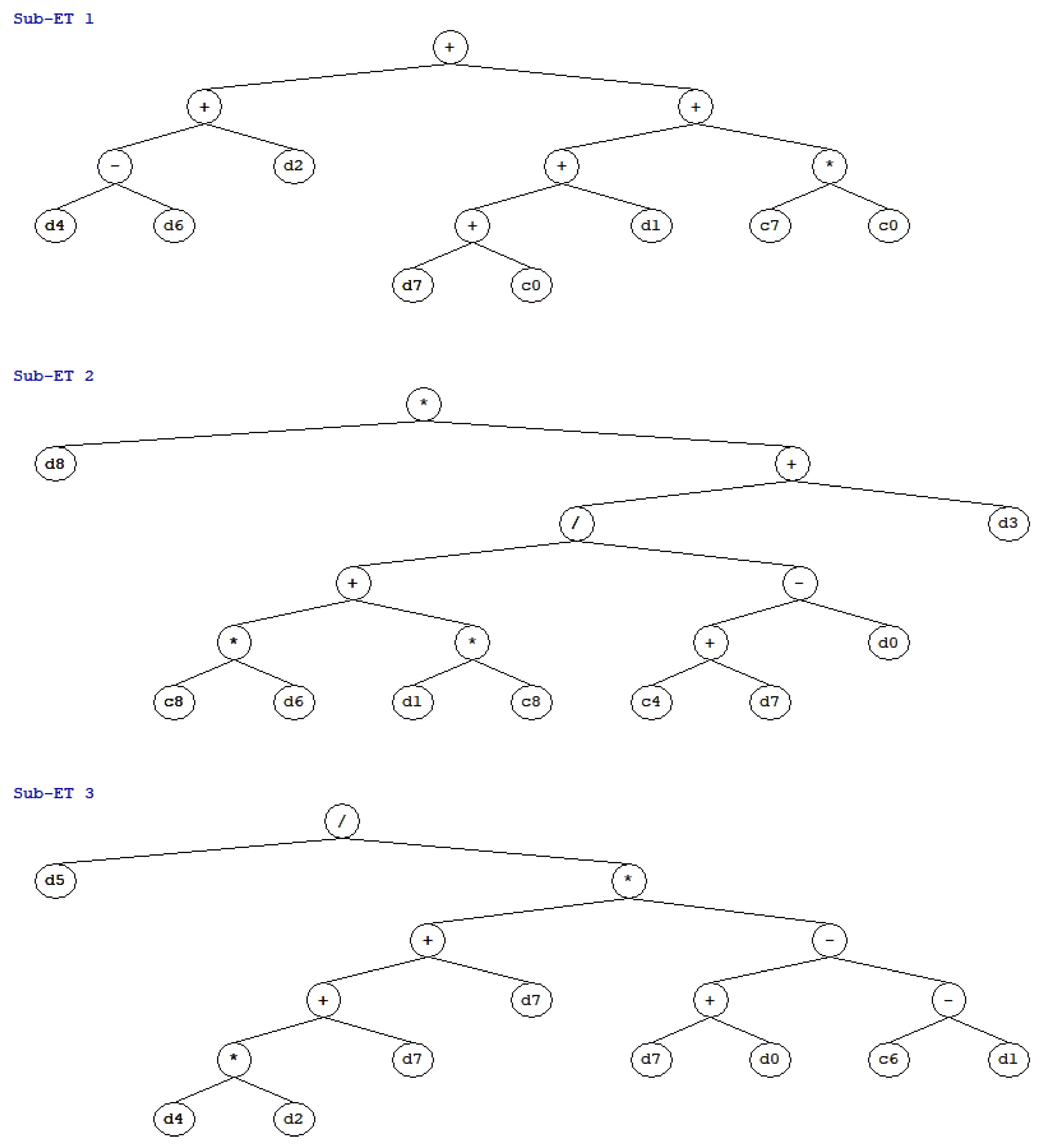
4.2. Gene Expression Programming
- Choosing a fitness function allowing the GEP to achieve an optimum solution by itself. Here, a fitness function equals to 1000 was used [79].
- Choosing a set of terminals that involve the explanatory variables considered for the prediction of response. This study uses nine different explanatory variables for the prediction of wear depth of concrete (explained in Section 3).
- Choosing the set of functions. To get a simple GEP equation, this research uses four basic arithmetical functions, i.e., and /.
- Choosing the architecture of chromosomes, i.e., the genes, head size, and linking function. To avoid complexity, in this research three genes with head size equal to ten and addition as a linking function were utilized.
- Choosing the set of genetic operators. A mixture of crossover, mutation, and transposition was used as a genetic operator.
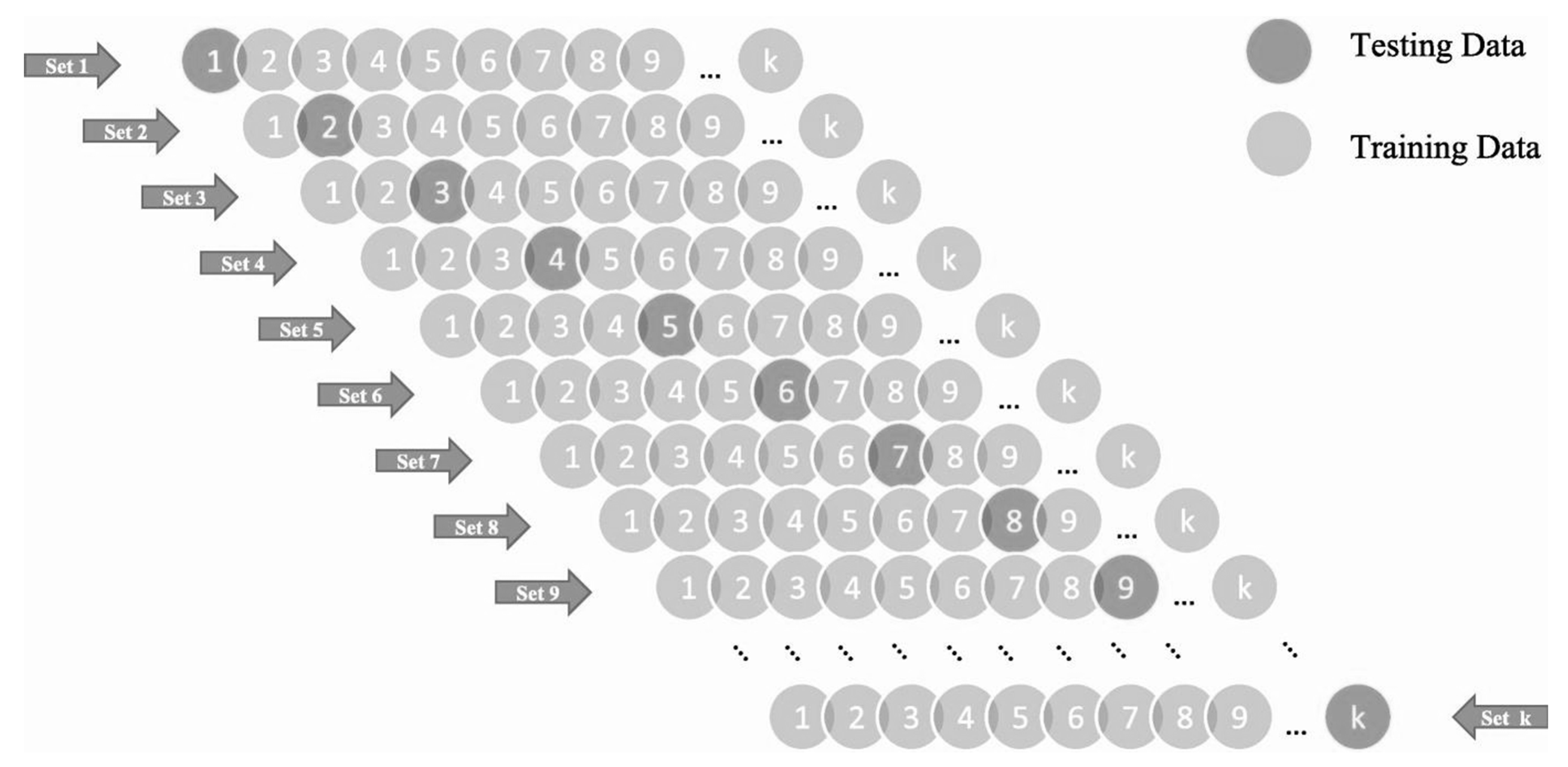
4.3. K-Fold Cross-Validation (KFCV) and Statistical Metrics
5. Result and Discusion
5.1. Random Forest Regression
5.2. Development of GEP Based Empirical Equation
5.3. Performance of GEP Model
5.4. K-Fold Cross Validation (KFCV)
6. Limitation and Recommendation for Future Study
7. Conclusions
- The results disclose that the RFR and GEP model can precisely and accurately estimate the DW exclusive of any prior assumption. Moreover, the DW estimation from GEP model is better than RFR based model. GEP technique delivers a simplified formula of DW with considerably greater accuracy between experimental and predicted outcome. This shows the diverse nature of GEP technique as it has space for non-linear and linear data.
- The performance of both models was testified via statistical metrics like R2, MAE, RMSE, RSE, RRMSE and performance index (ρ). The analysis of all metrics reveals that both the models deliver an outburst performance. The R2 of RFR and GEP model comes out to be 0.9523 and 0.9667 respectively. Since the ρ of predicted DW by RFR and GEP are lesser than 0.2 that is 0.0679 and 0.0501, respectively; so, both models can be categorized as good models. The models also meet the external validation criterion suggested in the previous literature.
- The validation via KFCV reveals that the model’s variables are highly correlated and accurate having a minimal error statistic between predicted DW and experimental results.
- The sensitivity analysis via GEP based formulation shows that the considered explanatory variables have an immense impact on the estimation of wear depth of concrete following the order: T (34.16%) > A (14.22%) > C (12.13%) > AE (9.914%) > W (8.834%) > F (6.551%) > P (5.221%) > FA (4.985%) > CA (3.986%).
- The simplified mathematical expression delivered by GEP algorithm for predicting the DW of fly-ash based concrete are much simpler. The established GEP equation is recommended to be utilized in the routine-based design practices rather than performing time-consuming and laborious experimental tests. It is noteworthy to mark that the projected equation is generally capable to predict the DW within the vast range of explanatory variables exercised during formulation. In addition, the results can be used to check the applicability of different mix design ratio of fly-ash concrete. The site engineer can design the required mix ratio keeping the cost of concrete as low as required with little or no help from the consultants.
Author Contributions
Funding
Institutional Review Board Statement
Informed Consent Statement
Data Availability Statement
Acknowledgments
Conflicts of Interest
Appendix A

| Sr.No. | Cement (kg/m3) | Fly Ash (kg/m3) | Water (kg/m3) | Fine Aggregate (kg/m3) | Coarse Aggregate (kg/m3) | Plasticizer (kg/m3) | Air Entraining (g/m3) | Age (Days) | Time of Testing (mins) | Depth of Wear (mm) |
|---|---|---|---|---|---|---|---|---|---|---|
| 1 | 398 | 0 | 123 | 715 | 1259 | 2.7 | 280 | 28 | 5 | 0.11 |
| 2 | 398 | 0 | 123 | 715 | 1259 | 2.7 | 280 | 28 | 10 | 0.26 |
| 3 | 398 | 0 | 123 | 715 | 1259 | 2.7 | 280 | 28 | 15 | 0.64 |
| 4 | 398 | 0 | 123 | 715 | 1259 | 2.7 | 280 | 28 | 20 | 1.04 |
| 5 | 398 | 0 | 123 | 715 | 1259 | 2.7 | 280 | 28 | 25 | 1.17 |
| 6 | 398 | 0 | 123 | 715 | 1259 | 2.7 | 280 | 28 | 30 | 1.45 |
| 7 | 398 | 0 | 123 | 715 | 1259 | 2.7 | 280 | 28 | 35 | 1.65 |
| 8 | 398 | 0 | 123 | 715 | 1259 | 2.7 | 280 | 28 | 40 | 1.88 |
| 9 | 398 | 0 | 123 | 715 | 1259 | 2.7 | 280 | 28 | 45 | 1.99 |
| 10 | 398 | 0 | 123 | 715 | 1259 | 2.7 | 280 | 28 | 50 | 2.17 |
| 11 | 398 | 0 | 123 | 715 | 1259 | 2.7 | 280 | 28 | 55 | 2.28 |
| 12 | 398 | 0 | 123 | 715 | 1259 | 2.7 | 280 | 28 | 60 | 2.42 |
| 13 | 397 | 0 | 125 | 712 | 1264 | 2.7 | 330 | 28 | 5 | 0.1 |
| 14 | 397 | 0 | 125 | 712 | 1264 | 2.7 | 330 | 28 | 10 | 0.26 |
| 15 | 397 | 0 | 125 | 712 | 1264 | 2.7 | 330 | 28 | 15 | 0.41 |
| 16 | 397 | 0 | 125 | 712 | 1264 | 2.7 | 330 | 28 | 20 | 0.63 |
| 17 | 397 | 0 | 125 | 712 | 1264 | 2.7 | 330 | 28 | 25 | 0.75 |
| 18 | 397 | 0 | 125 | 712 | 1264 | 2.7 | 330 | 28 | 30 | 0.88 |
| 19 | 397 | 0 | 125 | 712 | 1264 | 2.7 | 330 | 28 | 35 | 1.04 |
| 20 | 397 | 0 | 125 | 712 | 1264 | 2.7 | 330 | 28 | 40 | 1.21 |
| 21 | 397 | 0 | 125 | 712 | 1264 | 2.7 | 330 | 28 | 45 | 1.33 |
| 22 | 397 | 0 | 125 | 712 | 1264 | 2.7 | 330 | 28 | 50 | 1.5 |
| 23 | 397 | 0 | 125 | 712 | 1264 | 2.7 | 330 | 28 | 55 | 1.67 |
| 24 | 397 | 0 | 125 | 712 | 1264 | 2.7 | 330 | 28 | 60 | 1.85 |
| 25 | 375 | 0 | 135 | 682 | 1182 | 2.9 | 270 | 28 | 5 | 0.23 |
| 26 | 375 | 0 | 135 | 682 | 1182 | 2.9 | 270 | 28 | 10 | 0.46 |
| 27 | 375 | 0 | 135 | 682 | 1182 | 2.9 | 270 | 28 | 15 | 0.69 |
| 28 | 375 | 0 | 135 | 682 | 1182 | 2.9 | 270 | 28 | 20 | 0.82 |
| 29 | 375 | 0 | 135 | 682 | 1182 | 2.9 | 270 | 28 | 25 | 1.01 |
| 30 | 375 | 0 | 135 | 682 | 1182 | 2.9 | 270 | 28 | 30 | 1.11 |
| 31 | 375 | 0 | 135 | 682 | 1182 | 2.9 | 270 | 28 | 35 | 1.28 |
| 32 | 375 | 0 | 135 | 682 | 1182 | 2.9 | 270 | 28 | 40 | 1.39 |
| 33 | 375 | 0 | 135 | 682 | 1182 | 2.9 | 270 | 28 | 45 | 1.57 |
| 34 | 375 | 0 | 135 | 682 | 1182 | 2.9 | 270 | 28 | 50 | 1.75 |
| 35 | 375 | 0 | 135 | 682 | 1182 | 2.9 | 270 | 28 | 55 | 1.89 |
| 36 | 375 | 0 | 135 | 682 | 1182 | 2.9 | 270 | 28 | 60 | 2.06 |
| 37 | 328 | 72 | 139 | 695 | 1207 | 2.9 | 300 | 28 | 5 | 0.14 |
| 38 | 328 | 72 | 139 | 695 | 1207 | 2.9 | 300 | 28 | 10 | 0.36 |
| 39 | 328 | 72 | 139 | 695 | 1207 | 2.9 | 300 | 28 | 15 | 0.52 |
| 40 | 328 | 72 | 139 | 695 | 1207 | 2.9 | 300 | 28 | 20 | 0.7 |
| 41 | 328 | 72 | 139 | 695 | 1207 | 2.9 | 300 | 28 | 25 | 0.92 |
| 42 | 328 | 72 | 139 | 695 | 1207 | 2.9 | 300 | 28 | 30 | 1.08 |
| 43 | 328 | 72 | 139 | 695 | 1207 | 2.9 | 300 | 28 | 35 | 1.24 |
| 44 | 328 | 72 | 139 | 695 | 1207 | 2.9 | 300 | 28 | 40 | 1.39 |
| 45 | 328 | 72 | 139 | 695 | 1207 | 2.9 | 300 | 28 | 45 | 1.62 |
| 46 | 328 | 72 | 139 | 695 | 1207 | 2.9 | 300 | 28 | 50 | 1.78 |
| 47 | 328 | 72 | 139 | 695 | 1207 | 2.9 | 300 | 28 | 55 | 1.96 |
| 48 | 328 | 72 | 139 | 695 | 1207 | 2.9 | 300 | 28 | 60 | 2.16 |
| 49 | 259 | 139 | 133 | 677 | 1172 | 2.8 | 350 | 28 | 5 | 0.14 |
| 50 | 259 | 139 | 133 | 677 | 1172 | 2.8 | 350 | 28 | 10 | 0.34 |
| 51 | 259 | 139 | 133 | 677 | 1172 | 2.8 | 350 | 28 | 15 | 0.5 |
| 52 | 259 | 139 | 133 | 677 | 1172 | 2.8 | 350 | 28 | 20 | 0.66 |
| 53 | 259 | 139 | 133 | 677 | 1172 | 2.8 | 350 | 28 | 25 | 0.85 |
| 54 | 259 | 139 | 133 | 677 | 1172 | 2.8 | 350 | 28 | 30 | 1.02 |
| 55 | 259 | 139 | 133 | 677 | 1172 | 2.8 | 350 | 28 | 35 | 1.18 |
| 56 | 259 | 139 | 133 | 677 | 1172 | 2.8 | 350 | 28 | 40 | 1.33 |
| 57 | 259 | 139 | 133 | 677 | 1172 | 2.8 | 350 | 28 | 45 | 1.5 |
| 58 | 259 | 139 | 133 | 677 | 1172 | 2.8 | 350 | 28 | 50 | 1.74 |
| 59 | 259 | 139 | 133 | 677 | 1172 | 2.8 | 350 | 28 | 55 | 1.88 |
| 60 | 259 | 139 | 133 | 677 | 1172 | 2.8 | 350 | 28 | 60 | 2.05 |
| 61 | 320 | 71 | 129 | 693 | 1180 | 2.8 | 420 | 28 | 5 | 0.18 |
| 62 | 320 | 71 | 129 | 693 | 1180 | 2.8 | 420 | 28 | 10 | 0.32 |
| 63 | 320 | 71 | 129 | 693 | 1180 | 2.8 | 420 | 28 | 15 | 0.54 |
| 64 | 320 | 71 | 129 | 693 | 1180 | 2.8 | 420 | 28 | 20 | 0.64 |
| 65 | 320 | 71 | 129 | 693 | 1180 | 2.8 | 420 | 28 | 25 | 0.9 |
| 66 | 320 | 71 | 129 | 693 | 1180 | 2.8 | 420 | 28 | 30 | 1.03 |
| 67 | 320 | 71 | 129 | 693 | 1180 | 2.8 | 420 | 28 | 35 | 1.18 |
| 68 | 320 | 71 | 129 | 693 | 1180 | 2.8 | 420 | 28 | 40 | 1.33 |
| 69 | 320 | 71 | 129 | 693 | 1180 | 2.8 | 420 | 28 | 45 | 1.49 |
| 70 | 320 | 71 | 129 | 693 | 1180 | 2.8 | 420 | 28 | 50 | 1.65 |
| 71 | 320 | 71 | 129 | 693 | 1180 | 2.8 | 420 | 28 | 55 | 1.8 |
| 72 | 320 | 71 | 129 | 693 | 1180 | 2.8 | 420 | 28 | 60 | 1.95 |
| 73 | 398 | 0 | 123 | 715 | 1259 | 2.7 | 280 | 91 | 5 | 0.08 |
| 74 | 398 | 0 | 123 | 715 | 1259 | 2.7 | 280 | 91 | 10 | 0.23 |
| 75 | 398 | 0 | 123 | 715 | 1259 | 2.7 | 280 | 91 | 15 | 0.43 |
| 76 | 398 | 0 | 123 | 715 | 1259 | 2.7 | 280 | 91 | 20 | 0.55 |
| 77 | 398 | 0 | 123 | 715 | 1259 | 2.7 | 280 | 91 | 25 | 0.72 |
| 78 | 398 | 0 | 123 | 715 | 1259 | 2.7 | 280 | 91 | 30 | 0.94 |
| 79 | 398 | 0 | 123 | 715 | 1259 | 2.7 | 280 | 91 | 35 | 1.13 |
| 80 | 398 | 0 | 123 | 715 | 1259 | 2.7 | 280 | 91 | 40 | 1.27 |
| 81 | 398 | 0 | 123 | 715 | 1259 | 2.7 | 280 | 91 | 45 | 1.37 |
| 82 | 398 | 0 | 123 | 715 | 1259 | 2.7 | 280 | 91 | 50 | 1.5 |
| 83 | 398 | 0 | 123 | 715 | 1259 | 2.7 | 280 | 91 | 55 | 1.64 |
| 84 | 398 | 0 | 123 | 715 | 1259 | 2.7 | 280 | 91 | 60 | 1.8 |
| 85 | 397 | 0 | 125 | 712 | 1264 | 2.7 | 330 | 91 | 5 | 0.08 |
| 86 | 397 | 0 | 125 | 712 | 1264 | 2.7 | 330 | 91 | 10 | 0.23 |
| 87 | 397 | 0 | 125 | 712 | 1264 | 2.7 | 330 | 91 | 15 | 0.45 |
| 88 | 397 | 0 | 125 | 712 | 1264 | 2.7 | 330 | 91 | 20 | 0.62 |
| 89 | 397 | 0 | 125 | 712 | 1264 | 2.7 | 330 | 91 | 25 | 0.75 |
| 90 | 397 | 0 | 125 | 712 | 1264 | 2.7 | 330 | 91 | 30 | 0.9 |
| 91 | 397 | 0 | 125 | 712 | 1264 | 2.7 | 330 | 91 | 35 | 1.03 |
| 92 | 397 | 0 | 125 | 712 | 1264 | 2.7 | 330 | 91 | 40 | 1.12 |
| 93 | 397 | 0 | 125 | 712 | 1264 | 2.7 | 330 | 91 | 45 | 1.27 |
| 94 | 397 | 0 | 125 | 712 | 1264 | 2.7 | 330 | 91 | 50 | 1.41 |
| 95 | 397 | 0 | 125 | 712 | 1264 | 2.7 | 330 | 91 | 55 | 1.5 |
| 96 | 397 | 0 | 125 | 712 | 1264 | 2.7 | 330 | 91 | 60 | 1.63 |
| 97 | 375 | 0 | 135 | 682 | 1182 | 2.9 | 270 | 91 | 5 | 0.14 |
| 98 | 375 | 0 | 135 | 682 | 1182 | 2.9 | 270 | 91 | 10 | 0.29 |
| 99 | 375 | 0 | 135 | 682 | 1182 | 2.9 | 270 | 91 | 15 | 0.49 |
| 100 | 375 | 0 | 135 | 682 | 1182 | 2.9 | 270 | 91 | 20 | 0.75 |
| 101 | 375 | 0 | 135 | 682 | 1182 | 2.9 | 270 | 91 | 25 | 0.96 |
| 102 | 375 | 0 | 135 | 682 | 1182 | 2.9 | 270 | 91 | 30 | 1.1 |
| 103 | 375 | 0 | 135 | 682 | 1182 | 2.9 | 270 | 91 | 35 | 1.24 |
| 104 | 375 | 0 | 135 | 682 | 1182 | 2.9 | 270 | 91 | 40 | 1.39 |
| 105 | 375 | 0 | 135 | 682 | 1182 | 2.9 | 270 | 91 | 45 | 1.46 |
| 106 | 375 | 0 | 135 | 682 | 1182 | 2.9 | 270 | 91 | 50 | 1.58 |
| 107 | 375 | 0 | 135 | 682 | 1182 | 2.9 | 270 | 91 | 55 | 1.68 |
| 108 | 375 | 0 | 135 | 682 | 1182 | 2.9 | 270 | 91 | 60 | 1.77 |
| 109 | 328 | 72 | 139 | 695 | 1207 | 2.9 | 300 | 91 | 5 | 0.06 |
| 110 | 328 | 72 | 139 | 695 | 1207 | 2.9 | 300 | 91 | 10 | 0.26 |
| 111 | 328 | 72 | 139 | 695 | 1207 | 2.9 | 300 | 91 | 15 | 0.41 |
| 112 | 328 | 72 | 139 | 695 | 1207 | 2.9 | 300 | 91 | 20 | 0.62 |
| 113 | 328 | 72 | 139 | 695 | 1207 | 2.9 | 300 | 91 | 25 | 0.79 |
| 114 | 328 | 72 | 139 | 695 | 1207 | 2.9 | 300 | 91 | 30 | 0.94 |
| 115 | 328 | 72 | 139 | 695 | 1207 | 2.9 | 300 | 91 | 35 | 1.11 |
| 116 | 328 | 72 | 139 | 695 | 1207 | 2.9 | 300 | 91 | 40 | 1.27 |
| 117 | 328 | 72 | 139 | 695 | 1207 | 2.9 | 300 | 91 | 45 | 1.44 |
| 118 | 328 | 72 | 139 | 695 | 1207 | 2.9 | 300 | 91 | 50 | 1.53 |
| 119 | 328 | 72 | 139 | 695 | 1207 | 2.9 | 300 | 91 | 55 | 1.65 |
| 120 | 328 | 72 | 139 | 695 | 1207 | 2.9 | 300 | 91 | 60 | 1.75 |
| 121 | 259 | 139 | 133 | 677 | 1172 | 2.8 | 350 | 91 | 5 | 0.05 |
| 122 | 259 | 139 | 133 | 677 | 1172 | 2.8 | 350 | 91 | 10 | 0.17 |
| 123 | 259 | 139 | 133 | 677 | 1172 | 2.8 | 350 | 91 | 15 | 0.35 |
| 124 | 259 | 139 | 133 | 677 | 1172 | 2.8 | 350 | 91 | 20 | 0.53 |
| 125 | 259 | 139 | 133 | 677 | 1172 | 2.8 | 350 | 91 | 25 | 0.76 |
| 126 | 259 | 139 | 133 | 677 | 1172 | 2.8 | 350 | 91 | 30 | 0.9 |
| 127 | 259 | 139 | 133 | 677 | 1172 | 2.8 | 350 | 91 | 35 | 1.04 |
| 128 | 259 | 139 | 133 | 677 | 1172 | 2.8 | 350 | 91 | 40 | 1.18 |
| 129 | 259 | 139 | 133 | 677 | 1172 | 2.8 | 350 | 91 | 45 | 1.31 |
| 130 | 259 | 139 | 133 | 677 | 1172 | 2.8 | 350 | 91 | 50 | 1.48 |
| 131 | 259 | 139 | 133 | 677 | 1172 | 2.8 | 350 | 91 | 55 | 1.64 |
| 132 | 259 | 139 | 133 | 677 | 1172 | 2.8 | 350 | 91 | 60 | 1.7 |
| 133 | 320 | 71 | 129 | 693 | 1180 | 2.8 | 420 | 91 | 5 | 0.1 |
| 134 | 320 | 71 | 129 | 693 | 1180 | 2.8 | 420 | 91 | 10 | 0.27 |
| 135 | 320 | 71 | 129 | 693 | 1180 | 2.8 | 420 | 91 | 15 | 0.53 |
| 136 | 320 | 71 | 129 | 693 | 1180 | 2.8 | 420 | 91 | 20 | 0.64 |
| 137 | 320 | 71 | 129 | 693 | 1180 | 2.8 | 420 | 91 | 25 | 0.82 |
| 138 | 320 | 71 | 129 | 693 | 1180 | 2.8 | 420 | 91 | 30 | 0.99 |
| 139 | 320 | 71 | 129 | 693 | 1180 | 2.8 | 420 | 91 | 35 | 1.1 |
| 140 | 320 | 71 | 129 | 693 | 1180 | 2.8 | 420 | 91 | 40 | 1.26 |
| 141 | 320 | 71 | 129 | 693 | 1180 | 2.8 | 420 | 91 | 45 | 1.39 |
| 142 | 320 | 71 | 129 | 693 | 1180 | 2.8 | 420 | 91 | 50 | 1.5 |
| 143 | 320 | 71 | 129 | 693 | 1180 | 2.8 | 420 | 91 | 55 | 1.59 |
| 144 | 320 | 71 | 129 | 693 | 1180 | 2.8 | 420 | 91 | 60 | 1.71 |
| 145 | 398 | 0 | 123 | 715 | 1259 | 2.7 | 280 | 365 | 5 | 0.07 |
| 146 | 398 | 0 | 123 | 715 | 1259 | 2.7 | 280 | 365 | 10 | 0.19 |
| 147 | 398 | 0 | 123 | 715 | 1259 | 2.7 | 280 | 365 | 15 | 0.28 |
| 148 | 398 | 0 | 123 | 715 | 1259 | 2.7 | 280 | 365 | 20 | 0.37 |
| 149 | 398 | 0 | 123 | 715 | 1259 | 2.7 | 280 | 365 | 25 | 0.42 |
| 150 | 398 | 0 | 123 | 715 | 1259 | 2.7 | 280 | 365 | 30 | 0.56 |
| 151 | 398 | 0 | 123 | 715 | 1259 | 2.7 | 280 | 365 | 35 | 0.71 |
| 152 | 398 | 0 | 123 | 715 | 1259 | 2.7 | 280 | 365 | 40 | 0.84 |
| 153 | 398 | 0 | 123 | 715 | 1259 | 2.7 | 280 | 365 | 45 | 1.08 |
| 154 | 398 | 0 | 123 | 715 | 1259 | 2.7 | 280 | 365 | 50 | 1.19 |
| 155 | 398 | 0 | 123 | 715 | 1259 | 2.7 | 280 | 365 | 55 | 1.17 |
| 156 | 398 | 0 | 123 | 715 | 1259 | 2.7 | 280 | 365 | 60 | 1.44 |
| 157 | 397 | 0 | 125 | 712 | 1264 | 2.7 | 330 | 365 | 5 | 0.08 |
| 158 | 397 | 0 | 125 | 712 | 1264 | 2.7 | 330 | 365 | 10 | 0.24 |
| 159 | 397 | 0 | 125 | 712 | 1264 | 2.7 | 330 | 365 | 15 | 0.35 |
| 160 | 397 | 0 | 125 | 712 | 1264 | 2.7 | 330 | 365 | 20 | 0.49 |
| 161 | 397 | 0 | 125 | 712 | 1264 | 2.7 | 330 | 365 | 25 | 0.63 |
| 162 | 397 | 0 | 125 | 712 | 1264 | 2.7 | 330 | 365 | 30 | 0.76 |
| 163 | 397 | 0 | 125 | 712 | 1264 | 2.7 | 330 | 365 | 35 | 0.85 |
| 164 | 397 | 0 | 125 | 712 | 1264 | 2.7 | 330 | 365 | 40 | 0.96 |
| 165 | 397 | 0 | 125 | 712 | 1264 | 2.7 | 330 | 365 | 45 | 1.04 |
| 166 | 397 | 0 | 125 | 712 | 1264 | 2.7 | 330 | 365 | 50 | 1.17 |
| 167 | 397 | 0 | 125 | 712 | 1264 | 2.7 | 330 | 365 | 55 | 1.28 |
| 168 | 397 | 0 | 125 | 712 | 1264 | 2.7 | 330 | 365 | 60 | 1.36 |
| 169 | 375 | 0 | 135 | 682 | 1182 | 2.9 | 270 | 365 | 5 | 0.14 |
| 170 | 375 | 0 | 135 | 682 | 1182 | 2.9 | 270 | 365 | 10 | 0.22 |
| 171 | 375 | 0 | 135 | 682 | 1182 | 2.9 | 270 | 365 | 15 | 0.18 |
| 172 | 375 | 0 | 135 | 682 | 1182 | 2.9 | 270 | 365 | 20 | 0.4 |
| 173 | 375 | 0 | 135 | 682 | 1182 | 2.9 | 270 | 365 | 25 | 0.57 |
| 174 | 375 | 0 | 135 | 682 | 1182 | 2.9 | 270 | 365 | 30 | 0.64 |
| 175 | 375 | 0 | 135 | 682 | 1182 | 2.9 | 270 | 365 | 35 | 0.73 |
| 176 | 375 | 0 | 135 | 682 | 1182 | 2.9 | 270 | 365 | 40 | 0.78 |
| 177 | 375 | 0 | 135 | 682 | 1182 | 2.9 | 270 | 365 | 45 | 1.04 |
| 178 | 375 | 0 | 135 | 682 | 1182 | 2.9 | 270 | 365 | 50 | 1.11 |
| 179 | 375 | 0 | 135 | 682 | 1182 | 2.9 | 270 | 365 | 55 | 1.26 |
| 180 | 375 | 0 | 135 | 682 | 1182 | 2.9 | 270 | 365 | 60 | 1.43 |
| 181 | 328 | 72 | 139 | 695 | 1207 | 2.9 | 300 | 365 | 5 | 0.11 |
| 182 | 328 | 72 | 139 | 695 | 1207 | 2.9 | 300 | 365 | 10 | 0.35 |
| 183 | 328 | 72 | 139 | 695 | 1207 | 2.9 | 300 | 365 | 15 | 0.48 |
| 184 | 328 | 72 | 139 | 695 | 1207 | 2.9 | 300 | 365 | 20 | 0.6 |
| 185 | 328 | 72 | 139 | 695 | 1207 | 2.9 | 300 | 365 | 25 | 0.81 |
| 186 | 328 | 72 | 139 | 695 | 1207 | 2.9 | 300 | 365 | 30 | 0.93 |
| 187 | 328 | 72 | 139 | 695 | 1207 | 2.9 | 300 | 365 | 35 | 1.11 |
| 188 | 328 | 72 | 139 | 695 | 1207 | 2.9 | 300 | 365 | 40 | 1.3 |
| 189 | 328 | 72 | 139 | 695 | 1207 | 2.9 | 300 | 365 | 45 | 1.57 |
| 190 | 328 | 72 | 139 | 695 | 1207 | 2.9 | 300 | 365 | 50 | 1.71 |
| 191 | 328 | 72 | 139 | 695 | 1207 | 2.9 | 300 | 365 | 55 | 1.84 |
| 192 | 328 | 72 | 139 | 695 | 1207 | 2.9 | 300 | 365 | 60 | 1.94 |
| 193 | 259 | 139 | 133 | 677 | 1172 | 2.8 | 350 | 365 | 5 | 0.18 |
| 194 | 259 | 139 | 133 | 677 | 1172 | 2.8 | 350 | 365 | 10 | 0.47 |
| 195 | 259 | 139 | 133 | 677 | 1172 | 2.8 | 350 | 365 | 15 | 0.46 |
| 196 | 259 | 139 | 133 | 677 | 1172 | 2.8 | 350 | 365 | 20 | 0.62 |
| 197 | 259 | 139 | 133 | 677 | 1172 | 2.8 | 350 | 365 | 25 | 0.73 |
| 198 | 259 | 139 | 133 | 677 | 1172 | 2.8 | 350 | 365 | 30 | 0.9 |
| 199 | 259 | 139 | 133 | 677 | 1172 | 2.8 | 350 | 365 | 35 | 1.03 |
| 200 | 259 | 139 | 133 | 677 | 1172 | 2.8 | 350 | 365 | 40 | 1.19 |
| 201 | 259 | 139 | 133 | 677 | 1172 | 2.8 | 350 | 365 | 45 | 1.22 |
| 202 | 259 | 139 | 133 | 677 | 1172 | 2.8 | 350 | 365 | 50 | 1.37 |
| 203 | 259 | 139 | 133 | 677 | 1172 | 2.8 | 350 | 365 | 55 | 1.49 |
| 204 | 259 | 139 | 133 | 677 | 1172 | 2.8 | 350 | 365 | 60 | 1.5 |
| 205 | 320 | 71 | 129 | 693 | 1180 | 2.8 | 420 | 365 | 5 | 0.11 |
| 206 | 320 | 71 | 129 | 693 | 1180 | 2.8 | 420 | 365 | 10 | 0.28 |
| 207 | 320 | 71 | 129 | 693 | 1180 | 2.8 | 420 | 365 | 15 | 0.41 |
| 208 | 320 | 71 | 129 | 693 | 1180 | 2.8 | 420 | 365 | 20 | 0.65 |
| 209 | 320 | 71 | 129 | 693 | 1180 | 2.8 | 420 | 365 | 25 | 0.85 |
| 210 | 320 | 71 | 129 | 693 | 1180 | 2.8 | 420 | 365 | 30 | 1.02 |
| 211 | 320 | 71 | 129 | 693 | 1180 | 2.8 | 420 | 365 | 35 | 1.18 |
| 212 | 320 | 71 | 129 | 693 | 1180 | 2.8 | 420 | 365 | 40 | 1.24 |
| 213 | 320 | 71 | 129 | 693 | 1180 | 2.8 | 420 | 365 | 45 | 1.35 |
| 214 | 320 | 71 | 129 | 693 | 1180 | 2.8 | 420 | 365 | 50 | 1.49 |
| 215 | 320 | 71 | 129 | 693 | 1180 | 2.8 | 420 | 365 | 55 | 1.67 |
| 216 | 320 | 71 | 129 | 693 | 1180 | 2.8 | 420 | 365 | 60 | 1.81 |
References
- Adesina, A.; Awoyera, P.O.; Sivakrishna, A.; Kumar, K.R.; Gobinath, R. Phase change materials in concrete: An overview of properties. Mater. Today Proc. 2020, 27, 391–395. [Google Scholar] [CrossRef]
- Miller, D.; Doh, J.H.; Mulvey, M. Concrete slab comparison and embodied energy optimisation for alternate design and construction techniques. Constr. Build. Mater. 2015, 80, 329–338. [Google Scholar] [CrossRef] [Green Version]
- Shahmansouri, A.A.; Akbarzadeh Bengar, H.; AzariJafari, H. Life cycle assessment of eco-friendly concrete mixtures incorporating natural zeolite in sulfate-aggressive environment. Constr. Build. Mater. 2021, 268, 121136. [Google Scholar] [CrossRef]
- Raza, F.; Alshameri, B.; Jamil, S.M. Assessment of triple bottom line of sustainability for geotechnical projects. Environ. Dev. Sustain. 2021, 23, 4521–4558. [Google Scholar] [CrossRef]
- Palankar, N.; Ravi Shankar, A.U.; Mithun, B.M. Studies on eco-friendly concrete incorporating industrial waste as aggregates. Int. J. Sustain. Built Environ. 2015, 4, 378–390. [Google Scholar] [CrossRef] [Green Version]
- Akbar, A.; Farooq, F.; Shafique, M.; Aslam, F.; Alyousef, R.; Alabduljabbar, H. Sugarcane bagasse ash-based engineered geopolymer mortar incorporating propylene fibers. J. Build. Eng. 2021, 33, 101492. [Google Scholar] [CrossRef]
- Guo, M.; Hu, B.; Xing, F.; Zhou, X.; Sun, M.; Sui, L.; Zhou, Y. Characterization of the mechanical properties of eco-friendly concrete made with untreated sea sand and seawater based on statistical analysis. Constr. Build. Mater. 2020, 234, 117339. [Google Scholar] [CrossRef]
- Aslam, F.; Elkotb, M.A.; Iqtidar, A.; Khan, M.A.; Javed, M.F.; Usanova, K.I.; Khan, M.I.; Alamri, S.; Musarat, M.A. Compressive strength prediction of rice husk ash using multiphysics genetic expression programming. Ain Shams Eng. J. 2021, in press. [Google Scholar] [CrossRef]
- Jahanzaib Khalil, M.; Aslam, M.; Ahmad, S. Utilization of sugarcane bagasse ash as cement replacement for the production of sustainable concrete–A review. Constr. Build. Mater. 2020, 270, 121371. [Google Scholar] [CrossRef]
- Hemalatha, T.; Ramaswamy, A. A review on fly ash characteristics–Towards promoting high volume utilization in developing sustainable concrete. J. Clean. Prod. 2017, 147, 546–559. [Google Scholar] [CrossRef]
- Xu, G.; Shi, X. Characteristics and applications of fly ash as a sustainable construction material: A state-of-the-art review. Resour. Conserv. Recycl. 2018, 136, 95–109. [Google Scholar] [CrossRef]
- Bhatt, A.; Priyadarshini, S.; Acharath Mohanakrishnan, A.; Abri, A.; Sattler, M.; Techapaphawit, S. Physical, chemical, and geotechnical properties of coal fly ash: A global review. Case Stud. Constr. Mater. 2019, 11, e00263. [Google Scholar] [CrossRef]
- Li, B.; Hou, S.; Duan, Z.; Li, L.; Guo, W. Rheological behavior and compressive strength of concrete made with recycled fine aggregate of different size range. Constr. Build. Mater. 2021, 268, 121172. [Google Scholar] [CrossRef]
- Yi, Y.; Zhu, D.; Guo, S.; Zhang, Z.; Shi, C. A review on the deterioration and approaches to enhance the durability of concrete in the marine environment. Cem. Concr. Compos. 2020, 113, 103695. [Google Scholar] [CrossRef]
- Omoding, N.; Cunningham, L.S.; Lane-Serff, G.F. Effect of using recycled waste glass coarse aggregates on the hydrodynamic abrasion resistance of concrete. Constr. Build. Mater. 2021, 268, 121177. [Google Scholar] [CrossRef]
- Alaskar, A.; Alabduljabbar, H.; Mustafa Mohamed, A.; Alrshoudi, F.; Alyousef, R. Abrasion and skid resistance of concrete containing waste polypropylene fibers and palm oil fuel ash as pavement material. Constr. Build. Mater. 2021, 282, 122681. [Google Scholar] [CrossRef]
- Xu, O.; Han, S.; Liu, Y.; Li, C. Experimental investigation surface abrasion resistance and surface frost resistance of concrete pavement incorporating fly ash and slag. Int. J. Pavement Eng. 2020, 22, 1858–1866. [Google Scholar] [CrossRef]
- Tang, Y.; Feng, W.; Feng, W.; Chen, J.; Bao, D.; Li, L. Compressive properties of rubber-modified recycled aggregate concrete subjected to elevated temperatures. Constr. Build. Mater. 2021, 268, 121181. [Google Scholar] [CrossRef]
- Lau, C.K.; Lee, H.; Vimonsatit, V.; Huen, W.Y.; Chindaprasirt, P. Abrasion resistance behaviour of fly ash based geopolymer using nanoindentation and artificial neural network. Constr. Build. Mater. 2019, 212, 635–644. [Google Scholar] [CrossRef]
- Malazdrewicz, S.; Sadowski, Ł. An intelligent model for the prediction of the depth of the wear of cementitious composite modified with high-calcium fly ash. Compos. Struct. 2021, 259, 113234. [Google Scholar] [CrossRef]
- Sabarinathan, P.; Annamalai, V.E.; Sangeetha, P. Mechanical and Abrasion Resistance Properties of Concrete Containing Recycled Abrasive Waste as Partial Replacement of Fine Aggregate. Arab. J. Sci. Eng. 2021, 46, 10943–10952. [Google Scholar] [CrossRef]
- He, Z.; Chen, X.; Cai, X. Influence and mechanism of micro/nano-mineral admixtures on the abrasion resistance of concrete. Constr. Build. Mater. 2019, 197, 91–98. [Google Scholar] [CrossRef]
- Jain, A.; Siddique, S.; Gupta, T.; Sharma, R.K.; Chaudhary, S. Utilization of shredded waste plastic bags to improve impact and abrasion resistance of concrete. Environ. Dev. Sustain. 2020, 22, 337–362. [Google Scholar] [CrossRef]
- Adewuyi, A.P.; Sulaiman, I.A.; Akinyele, J.O. Compressive Strength and Abrasion Resistance of Concretes under Varying Exposure Conditions. Open J. Civ. Eng. 2017, 7, 82–99. [Google Scholar] [CrossRef] [Green Version]
- Wang, L.; Zhou, S.H.; Shi, Y.; Tang, S.W.; Chen, E. Effect of silica fume and PVA fiber on the abrasion resistance and volume stability of concrete. Compos. Part B Eng. 2017, 130, 28–37. [Google Scholar] [CrossRef]
- Jain, A.; Choudhary, R.; Gupta, R.; Chaudhary, S. Abrasion resistance and sorptivity characteristics of SCC containing granite waste. Mater. Today: Proc. 2020, 27, 524–528. [Google Scholar] [CrossRef]
- Yildizel, S.A.; Timur, O.; Ozturk, A.U. Abrasion Resistance and Mechanical Properties of Waste-Glass-Fiber-Reinforced Roller-compacted Concrete. Mech. Compos. Mater. 2018, 54, 251–256. [Google Scholar] [CrossRef]
- Nazari, A.; Riahi, S. Compressive strength and abrasion resistance of concrete containing SiO2 and Cr2O3 nanoparticles in different curing media. Mag. Concr. Res. 2012, 64, 177–188. [Google Scholar] [CrossRef]
- Li, H.; Zhang, M.H.; Ou, J.P. Abrasion resistance of concrete containing nano-particles for pavement. Wear 2006, 260, 1262–1266. [Google Scholar] [CrossRef]
- Chernysheva, N.; Lesovik, V.; Fediuk, R.; Vatin, N. Improvement of performances of the gypsum-cement fiber reinforced composite (GCFRC). Materials 2020, 13, 3847. [Google Scholar] [CrossRef]
- Tang, Y.; Feng, W.; Chen, Z.; Nong, Y.; Guan, S.; Sun, J. Fracture behavior of a sustainable material: Recycled concrete with waste crumb rubber subjected to elevated temperatures. J. Clean. Prod. 2021, 318, 128553. [Google Scholar] [CrossRef]
- Yunchao, T.; Zheng, C.; Wanhui, F.; Yumei, N.; Cong, L.; Jieming, C. Combined effects of nano-silica and silica fume on the mechanical behavior of recycled aggregate concrete. Nanotechnol. Rev. 2021, 10, 819–838. [Google Scholar] [CrossRef]
- Panda, S.; Sarkar, P.; Davis, R. Abrasion resistance and slake durability of copper slag aggregate concrete. J. Build. Eng. 2021, 35, 101987. [Google Scholar] [CrossRef]
- You, N.; Liu, Y.; Gu, D.; Ozbakkaloglu, T.; Pan, J.; Zhang, Y. Rheology, shrinkage and pore structure of alkali-activated slag-fly ash mortar incorporating copper slag as fine aggregate. Constr. Build. Mater. 2020, 242, 118029. [Google Scholar] [CrossRef]
- Farooq, F.; Akbar, A.; Khushnood, R.A.; Muhammad, W.L.B.; Rehman, S.K.U.; Javed, M.F. Experimental investigation of hybrid carbon nanotubes and graphite nanoplatelets on rheology, shrinkage, mechanical, and microstructure of SCCM. Materials 2020, 13, 230. [Google Scholar] [CrossRef] [Green Version]
- Babanajad, S.K.; Gandomi, A.H.; Mohammadzadeh, S.D.; Alavi, A.H. Numerical modeling of concrete strength under multiaxial confinement pressures using linear genetic programming. Autom. Constr. 2013, 36, 136–144. [Google Scholar] [CrossRef]
- Neira, P.; Bennun, L.; Pradena, M.; Gomez, J. Prediction of concrete compressive strength through artificial neural network. Gradjevinar 2020, 72, 585–592. [Google Scholar] [CrossRef]
- Han, Q.; Gui, C.; Xu, J.; Lacidogna, G. A generalized method to predict the compressive strength of high-performance concrete by improved random forest algorithm. Constr. Build. Mater. 2019, 226, 734–742. [Google Scholar] [CrossRef]
- Golafshani, E.M.; Behnood, A.; Arashpour, M. Predicting the compressive strength of normal and High-Performance Concretes using ANN and ANFIS hybridized with Grey Wolf Optimizer. Constr. Build. Mater. 2020, 232, 117266. [Google Scholar] [CrossRef]
- Bilim, C.; Atiş, C.D.; Tanyildizi, H.; Karahan, O. Predicting the compressive strength of ground granulated blast furnace slag concrete using artificial neural network. Adv. Eng. Softw. 2009, 40, 334–340. [Google Scholar] [CrossRef]
- Öztaş, A.; Pala, M.; Özbay, E.; Kanca, E.; Çaǧlar, N.; Bhatti, M.A. Predicting the compressive strength and slump of high strength concrete using neural network. Constr. Build. Mater. 2006, 20, 769–775. [Google Scholar] [CrossRef]
- Behnood, A.; Behnood, V.; Modiri Gharehveran, M.; Alyamac, K.E. Prediction of the compressive strength of normal and high-performance concretes using M5P model tree algorithm. Constr. Build. Mater. 2017, 142, 199–207. [Google Scholar] [CrossRef]
- Mousavi, S.M.; Aminian, P.; Gandomi, A.H.; Alavi, A.H.; Bolandi, H. A new predictive model for compressive strength of HPC using gene expression programming. Adv. Eng. Softw. 2012, 45, 105–114. [Google Scholar] [CrossRef]
- Behnood, A.; Golafshani, E.M. Predicting the compressive strength of silica fume concrete using hybrid artificial neural network with multi-objective grey wolves. J. Clean. Prod. 2018, 202, 54–64. [Google Scholar] [CrossRef]
- Golafshani, E.M.; Behnood, A. Estimating the optimal mix design of silica fume concrete using biogeography-based programming. Cem. Concr. Compos. 2019, 96, 95–105. [Google Scholar] [CrossRef]
- Özcan, F.; Atiş, C.D.; Karahan, O.; Uncuoǧlu, E.; Tanyildizi, H. Comparison of artificial neural network and fuzzy logic models for prediction of long-term compressive strength of silica fume concrete. Adv. Eng. Softw. 2009, 40, 856–863. [Google Scholar] [CrossRef]
- Golafshani, E.M.; Ashour, A. Prediction of self-compacting concrete elastic modulus using two symbolic regression techniques. Autom. Constr. 2016, 64, 7–19. [Google Scholar] [CrossRef] [Green Version]
- Farooq, F.; Czarnecki, S.; Niewiadomski, P.; Aslam, F.; Alabduljabbar, H.; Ostrowski, K.A.; Śliwa-Wieczorek, K.; Nowobilski, T.; Malazdrewicz, S. A comparative study for the prediction of the compressive strength of self-compacting concrete modified with fly ash. Materials 2021, 14, 4934. [Google Scholar] [CrossRef] [PubMed]
- Behnood, A.; Olek, J.; Glinicki, M.A. Predicting modulus elasticity of recycled aggregate concrete using M5′ model tree algorithm. Constr. Build. Mater. 2015, 94, 137–147. [Google Scholar] [CrossRef]
- Javed, M.F.; Farooq, F.; Memon, S.A.; Akbar, A.; Khan, M.A.; Aslam, F.; Alyousef, R.; Alabduljabbar, H.; Rehman, S.K.U.; Ur Rehman, S.K.; et al. New prediction model for the ultimate axial capacity of concrete-filled steel tubes: An evolutionary approach. Crystals 2020, 10, 741. [Google Scholar] [CrossRef]
- Erdal, H.I.; Karakurt, O.; Namli, E. High performance concrete compressive strength forecasting using ensemble models based on discrete wavelet transform. Eng. Appl. Artif. Intell. 2013, 26, 1246–1254. [Google Scholar] [CrossRef]
- Feng, D.C.; Liu, Z.T.; Wang, X.D.; Chen, Y.; Chang, J.Q.; Wei, D.F.; Jiang, Z.M. Machine learning-based compressive strength prediction for concrete: An adaptive boosting approach. Constr. Build. Mater. 2020, 230, 117000. [Google Scholar] [CrossRef]
- Kaloop, M.R.; Kumar, D.; Samui, P.; Hu, J.W.; Kim, D. Compressive strength prediction of high-performance concrete using gradient tree boosting machine. Constr. Build. Mater. 2020, 264, 120198. [Google Scholar] [CrossRef]
- Han, T.; Siddique, A.; Khayat, K.; Huang, J.; Kumar, A. An ensemble machine learning approach for prediction and optimization of modulus of elasticity of recycled aggregate concrete. Constr. Build. Mater. 2020, 244, 118271. [Google Scholar] [CrossRef]
- Zounemat-Kermani, M.; Stephan, D.; Barjenbruch, M.; Hinkelmann, R. Ensemble data mining modeling in corrosion of concrete sewer: A comparative study of network-based (MLPNN & RBFNN) and tree-based (RF, CHAID, & CART) models. Adv. Eng. Inform. 2020, 43, 101030. [Google Scholar] [CrossRef]
- Thai, D.-K.; Tu, M.; Bui, Q.; Bui, T.-T. Gradient tree boosting machine learning on predicting the failure modes of the RC panels under impact loads. Eng. Comput. 2019, 1, 3. [Google Scholar] [CrossRef]
- Zhang, J.; Ma, G.; Huang, Y.; Sun, J.; Aslani, F.; Nener, B. Modelling uniaxial compressive strength of lightweight self-compacting concrete using random forest regression. Constr. Build. Mater. 2019, 210, 713–719. [Google Scholar] [CrossRef]
- Sarir, P.; Chen, J.; Asteris, P.G.; Armaghani, D.J.; Tahir, M.M. Developing GEP tree-based, neuro-swarm, and whale optimization models for evaluation of bearing capacity of concrete-filled steel tube columns. Eng. Comput. 2021, 37, 1–19. [Google Scholar] [CrossRef]
- Ahmad, A.; Farooq, F.; Ostrowski, K.A.; Śliwa-Wieczorek, K.; Czarnecki, S. Application of novel machine learning techniques for predicting the surface chloride concentration in concrete containing waste material. Materials 2021, 14, 2297. [Google Scholar] [CrossRef]
- Gencel, O.; Kocabas, F.; Gok, M.S.; Koksal, F. Comparison of artificial neural networks and general linear model approaches for the analysis of abrasive wear of concrete. Constr. Build. Mater. 2011, 25, 3486–3494. [Google Scholar] [CrossRef]
- Murad, Y.; Tarawneh, A.; Arar, F.; Al-Zu’bi, A.; Al-Ghwairi, A.; Al-Jaafreh, A.; Tarawneh, M. Flexural strength prediction for concrete beams reinforced with FRP bars using gene expression programming. Structures 2021, 33, 3163–3172. [Google Scholar] [CrossRef]
- Yaseen, Z.M.; Tran, M.T.; Kim, S.; Bakhshpoori, T.; Deo, R.C. Shear strength prediction of steel fiber reinforced concrete beam using hybrid intelligence models: A new approach. Eng. Struct. 2018, 177, 244–255. [Google Scholar] [CrossRef]
- Nguyen, T.D.; Tran, T.H.; Hoang, N.D. Prediction of interface yield stress and plastic viscosity of fresh concrete using a hybrid machine learning approach. Adv. Eng. Inform. 2020, 44, 101057. [Google Scholar] [CrossRef]
- Murali, G.; Fediuk, R. A Taguchi approach for study on impact response of ultra-high-performance polypropylene fibrous cementitious composite. J. Build. Eng. 2020, 30, 101301. [Google Scholar] [CrossRef]
- Corotis, R.B. Probability and statistics in Civil Engineering. Struct. Saf. 1988, 5, 321. [Google Scholar] [CrossRef]
- Ahmad, A.; Farooq, F.; Niewiadomski, P.; Ostrowski, K.; Akbar, A.; Aslam, F.; Alyousef, R. Prediction of compressive strength of fly ash based concrete using individual and ensemble algorithm. Materials 2021, 14, 794. [Google Scholar] [CrossRef] [PubMed]
- Javed, M.F.; Amin, M.N.; Shah, M.I.; Khan, K.; Iftikhar, B.; Farooq, F.; Aslam, F.; Alyousef, R.; Alabduljabbar, H. Applications of gene expression programming and regression techniques for estimating compressive strength of bagasse ash based concrete. Crystals 2020, 10, 737. [Google Scholar] [CrossRef]
- Farooq, F.; Ahmed, W.; Akbar, A.; Aslam, F.; Alyousef, R. Predictive modeling for sustainable high-performance concrete from industrial wastes: A comparison and optimization of models using ensemble learners. J. Clean. Prod. 2021, 292, 126032. [Google Scholar] [CrossRef]
- Anjum, S. Impact of internship programs on professional and personal development of business students: A case study from Pakistan. Future Bus. J. 2020, 6, 2. [Google Scholar] [CrossRef] [Green Version]
- Kline, R.B. Principles and Practice of Structural Equation Modelling, 4th ed; Guilford Publication: New York, NY, USA, 2015. [Google Scholar]
- Schapire, R.E.; Freund, Y.; Bartlett, P.; Lee, W.S. Boosting the margin: A new explanation for the effectiveness of voting methods. Ann. Stat. 1998, 26, 1651–1686. [Google Scholar] [CrossRef]
- Breiman, L. Bagging predictors. Mach. Learn. 1996, 24, 123–140. [Google Scholar] [CrossRef] [Green Version]
- Breiman, L. Random forests. Mach. Learn. 2001, 45, 5–32. [Google Scholar] [CrossRef] [Green Version]
- Khan, M.A.; Memon, S.A.; Farooq, F.; Javed, M.F.; Aslam, F.; Alyousef, R. Compressive Strength of Fly-Ash-Based Geopolymer Concrete by Gene Expression Programming and Random Forest. Adv. Civ. Eng. 2021, 2021, 6618407. [Google Scholar] [CrossRef]
- Aslam, F.; Farooq, F.; Amin, M.N.; Khan, K.; Waheed, A.; Akbar, A.; Javed, M.F.; Alyousef, R.; Alabdulijabbar, H. Applications of Gene Expression Programming for Estimating Compressive Strength of High-Strength Concrete. Adv. Civ. Eng. 2020, 2020, 8850535. [Google Scholar] [CrossRef]
- Azim, I.; Yang, J.; Javed, M.F.; Iqbal, M.F.; Mahmood, Z.; Wang, F.; Liu, Q. feng Prediction model for compressive arch action capacity of RC frame structures under column removal scenario using gene expression programming. Structures 2020, 25, 212–228. [Google Scholar] [CrossRef]
- Iqbal, M.F.; Liu, Q.-F.; Azim, I.; Zhu, X.; Yang, J.; Javed, M.F.; Rauf, M. Prediction of mechanical properties of green concrete incorporating waste foundry sand based on gene expression programming. J. Hazard. Mater. 2020, 384, 121322. [Google Scholar] [CrossRef]
- Shahmansouri, A.A.; Akbarzadeh Bengar, H.; Ghanbari, S. Compressive strength prediction of eco-efficient GGBS-based geopolymer concrete using GEP method. J. Build. Eng. 2020, 31, 101326. [Google Scholar] [CrossRef]
- Saud, S.; Jamil, B.; Upadhyay, Y.; Irshad, K. Performance improvement of empirical models for estimation of global solar radiation in India: A k-fold cross-validation approach. Sustain. Energy Technol. Assess. 2020, 40, 100768. [Google Scholar] [CrossRef]
- Kohavi, R. A Study of Cross-Validation and Bootstrap for Accuracy Estimation and Model Selection. Int. Jt. Conf. Artif. Intell. 1995, 14, 1137–1145. [Google Scholar]
- Nguyen, T.; Kashani, A.; Ngo, T.; Bordas, S. Deep neural network with high-order neuron for the prediction of foamed concrete strength. Comput. Civ. Infrastruct. Eng. 2019, 34, 316–332. [Google Scholar] [CrossRef]
- Gandomi, A.H.; Alavi, A.H.; Mirzahosseini, M.R.; Nejad, F.M. Nonlinear Genetic-Based Models for Prediction of Flow Number of Asphalt Mixtures. J. Mater. Civ. Eng. 2011, 23, 248–263. [Google Scholar] [CrossRef]
- Jalal, F.E.; Xu, Y.; Iqbal, M.; Javed, M.F.; Jamhiri, B. Predictive modeling of swell-strength of expansive soils using artificial intelligence approaches: ANN, ANFIS and GEP. J. Environ. Manag. 2021, 289, 112420. [Google Scholar] [CrossRef] [PubMed]
- Despotovic, M.; Nedic, V.; Despotovic, D.; Cvetanovic, S. Evaluation of empirical models for predicting monthly mean horizontal diffuse solar radiation. Renew. Sustain. Energy Rev. 2016, 56, 246–260. [Google Scholar] [CrossRef]
- Gandomi, A.H.; Faramarzifar, A.; Rezaee, P.G.; Asghari, A.; Talatahari, S. New design equations for elastic modulus of concrete using multi expression programming. J. Civ. Eng. Manag. 2015, 21, 761–774. [Google Scholar] [CrossRef] [Green Version]
- Golbraikh, A.; Tropsha, A. Beware of q2! J. Mol. Graph. Model. 2002, 20, 269–276. [Google Scholar] [CrossRef]
- Roy, P.P.; Roy, K. On some aspects of variable selection for partial least squares regression models. QSAR Comb. Sci. 2008, 27, 302–313. [Google Scholar] [CrossRef]
- Khan, M.A.; Zafar, A.; Akbar, A.; Javed, M.F.; Mosavi, A. Application of gene expression programming (GEP) for the prediction of compressive strength of geopolymer concrete. Materials 2021, 14, 1106. [Google Scholar] [CrossRef]
- Rius, F.X. The Data Analysis Handbook. Chemom. Intell. Lab. Syst. 1995, 29, 327. [Google Scholar] [CrossRef]


| S.No | Waste Material | Property Studied | Conclusive Remarks | Reference |
|---|---|---|---|---|
| 1 | Super fine slag (SFS), nano-SiO2 (NS), fly ash (FA) | Abrasion resistance and microstructure of concrete. | Maximum enhancement in strength with 82%, 73% and 68% for surface mortar layer and 20%, 16% and 13% for concrete. | [22] |
| 2 | Shredded plastic waste bags | Density, abrasion resistance, compressive strength, workability and flexural strength. | Abrasion resistance, impact resistance and energy absorption increase. However compressive, flexural strength decreases. | [23] |
| 3 | Crushed granite coarse aggregate | Compressive strength and abrasion resistance | Coarse aggregate with 45% by mass content of cement show better performance as compared to fine aggregate with 28.7%. | [24] |
| 4 | Silica fume and PVA fiber | Tensile and compressive strength, abrasion resistance, volume stability and drying shrinkage | Addition of silica fume and PVA fiber shows enhancement in compressive strength and abrasion resistance. | [25] |
| 5 | Granite waste (GW) | Compressive strength and abrasion resistance | Significant enhancement is observed in compressive and abrasion resistance of self-compacting concrete. | [26] |
| 6 | Waste glass fiber (WGF) | Mechanical and abrasion resistance | Addition of 2% WFG yield maximum strength mechanism of rolled compacted concrete. | [27] |
| 7 | Nano size particles (silicon dioxide and Chromium oxide) | Abrasion resistance and compressive strength | Improvement in abrasion resistance is observed in both cured saturated lime water and in water. However, sample containing SiO2 show much more abrasion resistance as compared to other specimens. | [28] |
| 8 | Polypropylene fibers (PP), nano-silica (SiO2), and nano titanium oxide (TiO2) | Abrasion resistance of pavement concrete | Nanoparticles show maximum improvement. Furthermore, titanium oxide (TiO2) show an overall enhancement response in specimen of pavement concrete. | [29] |
| 9 | Waste polypropylene fibers (PP) and palm oil fuel ash (POFA) | Abrasion and skid resistance of pavement concrete | Intrusion of PP show decrease in compressive strength by 17% with enhancement in abrasion resistance by 25% is observed. | [16] |
| 10 | Copper slag as fine aggregate | Copper slag concrete | Improvement is observed by using cooper slag in concrete. | [33] |
| S.No | Concrete Type | Properties | Techniques | References |
|---|---|---|---|---|
| 1 | Normal concrete | Compressive strength | Genetic programming | [37] |
| ANN | [38] | |||
| 2 | High-performance concrete | Compressive strength | Random forest | [39] |
| ANN | [40,41,42] | |||
| M5P | [43] | |||
| Gene expression programming | [44] | |||
| 3 | Silica fume concrete | Compressive strength | Hybrid ANN | [45] |
| Biogeography-based programming (BBP) | [46] | |||
| ANN and ANFIS | [47] | |||
| 4 | Self-compacting concrete | Modulus of Elasticity | Biogeography-based programming (BBP) | [48] |
| Compressive strength | Artificial neuron network (ANN) and gene expression programming (GEP) | [49] | ||
| 5 | Recycled aggregate concrete | Modulus of Elasticity | M5P | [50] |
| 6 | Concrete filled steel tube | Compressive strength | GEP | [51] |
| 7 | High-performance concrete | Compressive strength | BANN | [52] |
| GBANN | ||||
| Adaptive boosting | [53] | |||
| RF | [39] | |||
| Gradient tree boosting | [54] | |||
| 8 | Recycled aggregate concrete | Modulus of Elasticity | RF+SVM | [55] |
| 9 | Corrosion of concrete sewer | Microbially induced concrete corrosion | Bagging/Boosting MLPNN/RBFNN/CHAID/CART | [56] |
| 10 | corrosion of concrete sewer | Microbially induced concrete corrosion | Ensemble RF | [56] |
| 11 | RC panels | Failure modes | GBML | [57] |
| 12 | Lightweight self-compacting concrete | Compressive strength | RF | [58] |
| 13 | Concrete filled steel tube | Bearing capacity | Gene expression programming | [59] |
| 14 | Concrete Containing Waste Material | Surface Chloride Concentration | Gene expression programming, Artificial neural network, Decision tree | [60] |
| 15 | Concrete with high calcium fly ash | Depth of wear of cement composite | Artificial neuron network | [20] |
| 16 | Concrete | Abrasive wear | Artificial neuron network and general linear model | [61] |
| 17 | Beam reinforced with FRP bars | Flexural strength | Gene expression programming | [62] |
| 18 | Fiber concrete beam | Shear strength | Particle Swarm Optimization | [63] |
| 19 | Fresh concrete | Yield stress and plastic viscosity | Particle swarm optimization and least squares support vector machine and | [64] |
| 20 | Ultra-high performance propylene-fiberious cementicious composites (UHPPFCC) | Compressive strength and impact energy | Taguchi approach | [65] |
| C | F | W | FA | CA | P | AE | A | T | DW | |
|---|---|---|---|---|---|---|---|---|---|---|
| C | 1 | |||||||||
| F | −0.787 | 1 | ||||||||
| W | −0.525 | 0.461 | 1 | |||||||
| FA | 0.754 | −0.645 | −0.732 | 1 | ||||||
| CA | 0.774 | −0.666 | −0.689 | 0.750 | 1 | |||||
| P | −0.379 | 0.282 | 0.750 | −0.727 | −0.729 | 1 | ||||
| AE | −0.524 | 0.532 | −0.136 | −0.174 | −0.362 | −0.161 | 1 | |||
| A | 0 | 0 | 0 | 0 | 0 | 0 | 0 | 1 | ||
| T | 0 | 0 | 0 | 0 | 0 | 0 | 0 | 0 | 1 | |
| DW | −0.032 | 0.032 | 0.046 | −0.022 | −0.039 | −0.052 | −0.005 | −0.191 | 0.737 | 1 |
| Parameters | Kurtosis | Skewness | Mean | Median | Mode | Minimum | Maximum | SD |
|---|---|---|---|---|---|---|---|---|
| Explanatory | ||||||||
| C (kg/m3) | −0.97 | −0.54 | 346.17 | 351.50 | 398.00 | 259.00 | 398.00 | 49.64 |
| F (kg/m3) | −1.03 | 0.59 | 47.00 | 35.50 | 0.00 | 0.00 | 139.00 | 52.23 |
| W (kg/m3) | −1.35 | 0.03 | 130.67 | 131.00 | 123.00 | 123.00 | 139.00 | 5.60 |
| FA (kg/m3) | −1.43 | 0.15 | 695.67 | 694.00 | 715.00 | 677.00 | 715.00 | 14.00 |
| CA (kg/m3) | −1.55 | 0.49 | 1210.67 | 1194.50 | 1259.00 | 1172.00 | 1264.00 | 37.62 |
| P (kg·L/m3) | −1.51 | 0.00 | 2.80 | 2.80 | 2.70 | 2.70 | 2.90 | 0.08 |
| AE (kg·mL/m3) | −0.55 | 0.78 | 325.00 | 315.00 | 280.00 | 270.00 | 420.00 | 50.70 |
| A (days) | −1.51 | 0.61 | 161.33 | 91.00 | 28.00 | 28.00 | 365.00 | 146.63 |
| T (min) | −1.22 | 0.00 | 32.50 | 32.50 | 5.00 | 5.00 | 60.00 | 17.30 |
| Response | ||||||||
| DW (mm) | −0.89 | 0.11 | 1.00 | 1.03 | 1.50 | 0.05 | 2.42 | 0.56 |
| Equations | Condition | Recommended by |
|---|---|---|
| 0.85 < k < 1.15 | [87] | |
| 0.85 < k′ < 1.15 | [87] | |
| Rm > 0.5 | [88] | |
| where | ||
| K-Fold | RFR Model | GEP Model | ||||||
|---|---|---|---|---|---|---|---|---|
| R2 | MAE (mm) | RMSE (mm) | MSE (mm) | R2 | MAE (mm) | RMSE (mm) | MSE (mm) | |
| 1 | 0.9186 | 0.13195 | 0.20130 | 0.00169 | 0.9354 | 0.05727 | 0.09130 | 0.00916 |
| 2 | 0.8693 | 0.15670 | 0.19173 | 0.07457 | 0.8592 | 0.12950 | 0.17166 | 0.02429 |
| 3 | 0.9393 | 0.12563 | 0.19590 | 0.03876 | 0.8436 | 0.13900 | 0.19770 | 0.03682 |
| 4 | 0.9764 | 0.10530 | 0.21984 | 0.05693 | 0.8656 | 0.14264 | 0.20269 | 0.04257 |
| 5 | 0.8654 | 0.18059 | 0.19959 | 0.00561 | 0.9198 | 0.13376 | 0.18250 | 0.03881 |
| 6 | 0.8892 | 0.01179 | 0.10130 | 0.01567 | 0.9953 | 0.03065 | 0.05653 | 0.00172 |
| 7 | 0.8544 | 0.13570 | 0.20250 | 0.01342 | 0.9174 | 0.11553 | 0.14255 | 0.01520 |
| 8 | 0.8446 | 0.19063 | 0.21056 | 0.06876 | 0.8762 | 0.15620 | 0.17543 | 0.03204 |
| 9 | 0.9065 | 0.04580 | 0.09640 | 0.05016 | 0.8575 | 0.10068 | 0.16461 | 0.02551 |
| 10 | 0.9085 | 0.06039 | 0.16246 | 0.00364 | 0.9509 | 0.12297 | 0.16246 | 0.03225 |
| Maximum | 0.9764 | 0.19063 | 0.21984 | 0.07457 | 0.9953 | 0.15620 | 0.20269 | 0.04257 |
| Minimum | 0.8446 | 0.01179 | 0.09640 | 0.00169 | 0.8436 | 0.03065 | 0.05653 | 0.00172 |
| Mean | 0.8972 | 0.11445 | 0.17816 | 0.03292 | 0.9021 | 0.11282 | 0.15474 | 0.02584 |
| Developed Models | R2 | MAE (mm) | RMSE (mm) | RRMSE | RSE (mm) | Sigma |
|---|---|---|---|---|---|---|
| GEP | 0.9667 | 0.07361 | 0.10631 | 0.09947 | 0.033263 | 0.050157 |
| RFR | 0.9523 | 0.08511 | 0.13420 | 0.13420 | 0.05062 | 0.067919 |
| Suggested Metric | RFR Model | GEP Model |
|---|---|---|
| 0.97635 | 0.99213 | |
| 1.0107 | 1.0000 | |
| 0.74995 | 0.791307 | |
| 0.9975 | 0.999715 | |
| 0.9491 | 0.96597 |
Publisher’s Note: MDPI stays neutral with regard to jurisdictional claims in published maps and institutional affiliations. |
© 2021 by the authors. Licensee MDPI, Basel, Switzerland. This article is an open access article distributed under the terms and conditions of the Creative Commons Attribution (CC BY) license (https://creativecommons.org/licenses/by/4.0/).
Share and Cite
Khan, M.A.; Farooq, F.; Javed, M.F.; Zafar, A.; Ostrowski, K.A.; Aslam, F.; Malazdrewicz, S.; Maślak, M. Simulation of Depth of Wear of Eco-Friendly Concrete Using Machine Learning Based Computational Approaches. Materials 2022, 15, 58. https://doi.org/10.3390/ma15010058
Khan MA, Farooq F, Javed MF, Zafar A, Ostrowski KA, Aslam F, Malazdrewicz S, Maślak M. Simulation of Depth of Wear of Eco-Friendly Concrete Using Machine Learning Based Computational Approaches. Materials. 2022; 15(1):58. https://doi.org/10.3390/ma15010058
Chicago/Turabian StyleKhan, Mohsin Ali, Furqan Farooq, Mohammad Faisal Javed, Adeel Zafar, Krzysztof Adam Ostrowski, Fahid Aslam, Seweryn Malazdrewicz, and Mariusz Maślak. 2022. "Simulation of Depth of Wear of Eco-Friendly Concrete Using Machine Learning Based Computational Approaches" Materials 15, no. 1: 58. https://doi.org/10.3390/ma15010058