
Development of VUMAT and VUHARD Subroutines for Simulating the Dynamic Mechanical Properties of Additively Manufactured Parts


Abstract
:1. Introduction
2. A Microstructure and Dislocation-Based Model for DMLS Ti6Al4V (ELI)
3. Materials and Methods
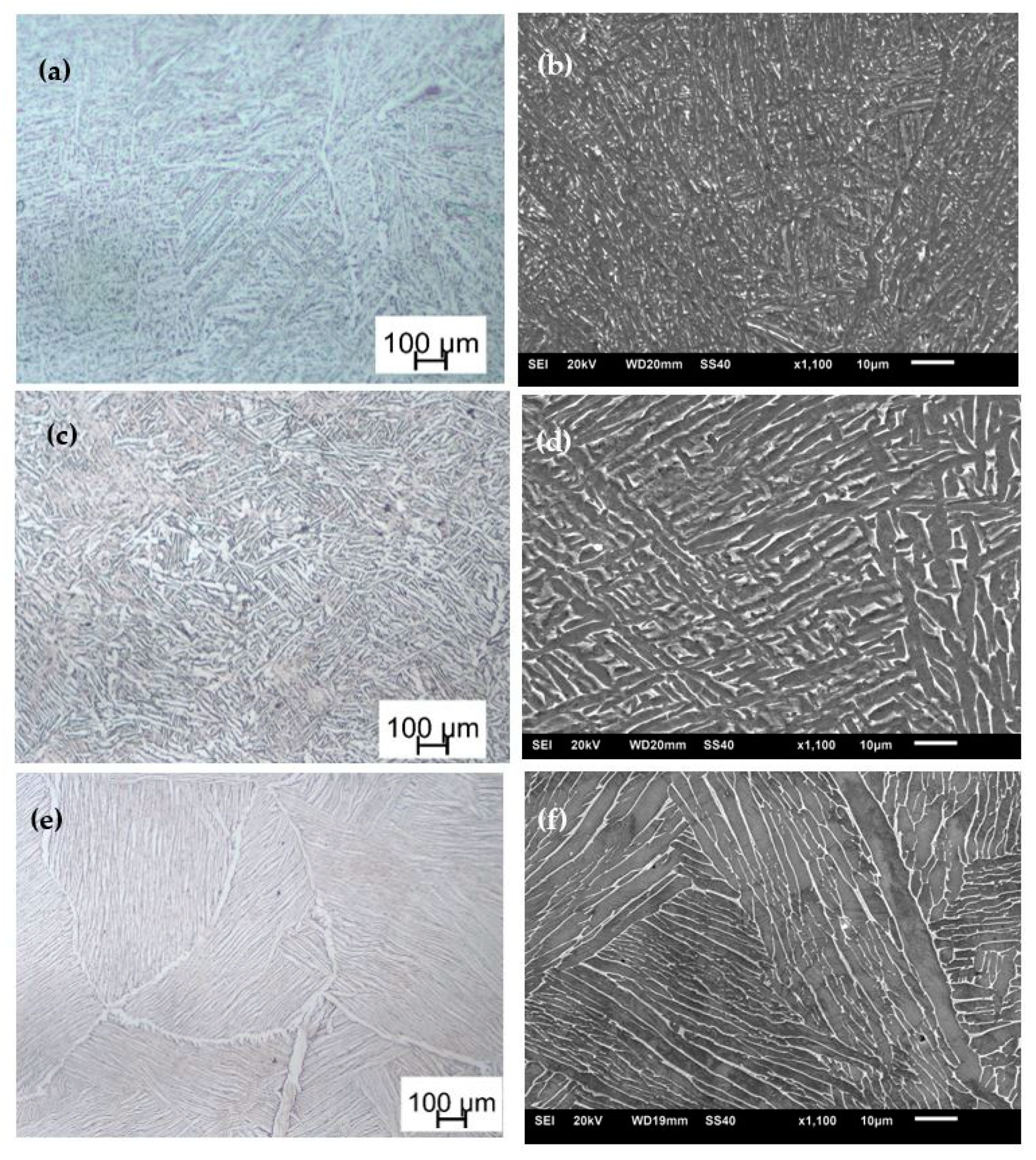
3.1. Materials
3.2. Experimental Tests
4. Implementation of Subroutines
4.1. Implementation of the Microstructure-Based Constitutive Flow Stress Model as a VUHARD Subroutine
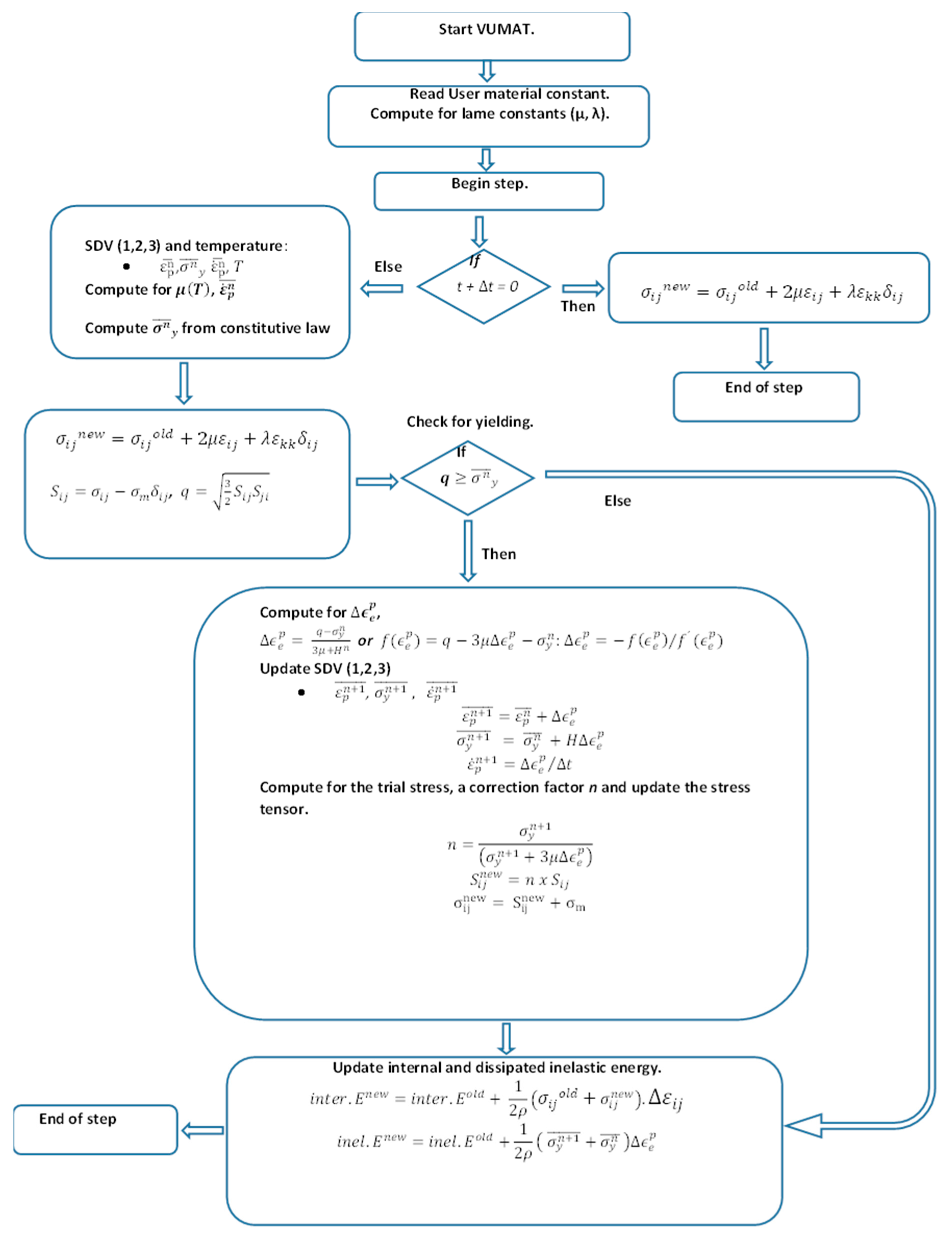
4.2. Implementation of the Microstructure-Based Constitutive Flow Stress Model as a VUMAT Subroutine
- ▪
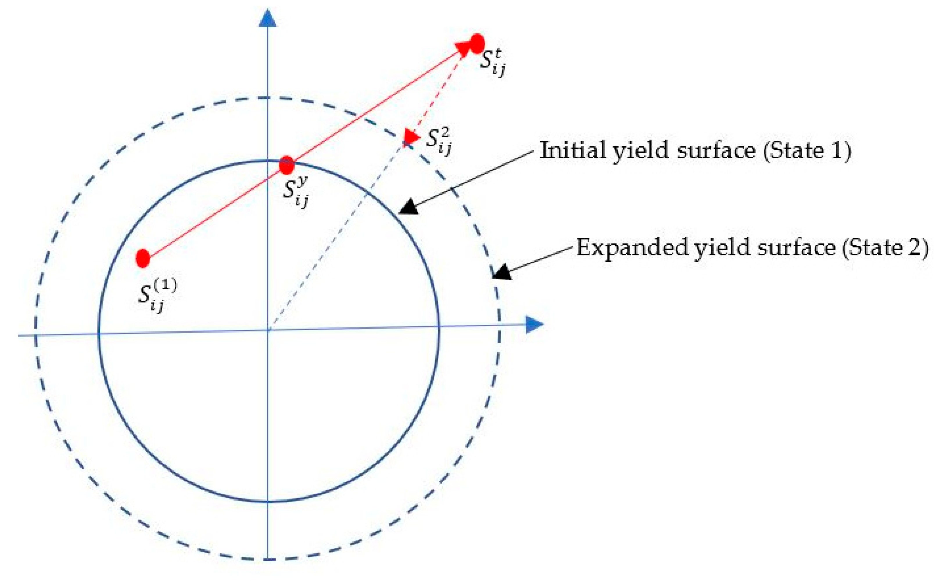
- If , then the state response was elastic, and the radial return algorithm that is inherent in the subroutine to correct the plastic response was skipped. The stress tensor and related deviatoric stress remain unchanged at any value of q. Therefore, the last step of the algorithm to compute internal energy and dissipation of inelastic energy was initiated. It is important to note that internal energy, abbreviated as ALLIE in ABAQUS, is the sum of the recoverable elastic strain energy and the energy dissipated through plastic deformation [27]. Since there was no plastic deformation, the inelastic energy remained zero, and the internal energy only included the elastic strain energy component.
- ▪
- If , then the stress state was outside the yield surface and was plastic. Thus, the radial return mapping previously described in Appendix A was initiated to compute the equivalent plastic strain and therefore return the predicted stress back to the expanded yield surface of the material. At this stage, strain hardening was expected since the loading was beyond the elastic limit.
5. Results and Discussions
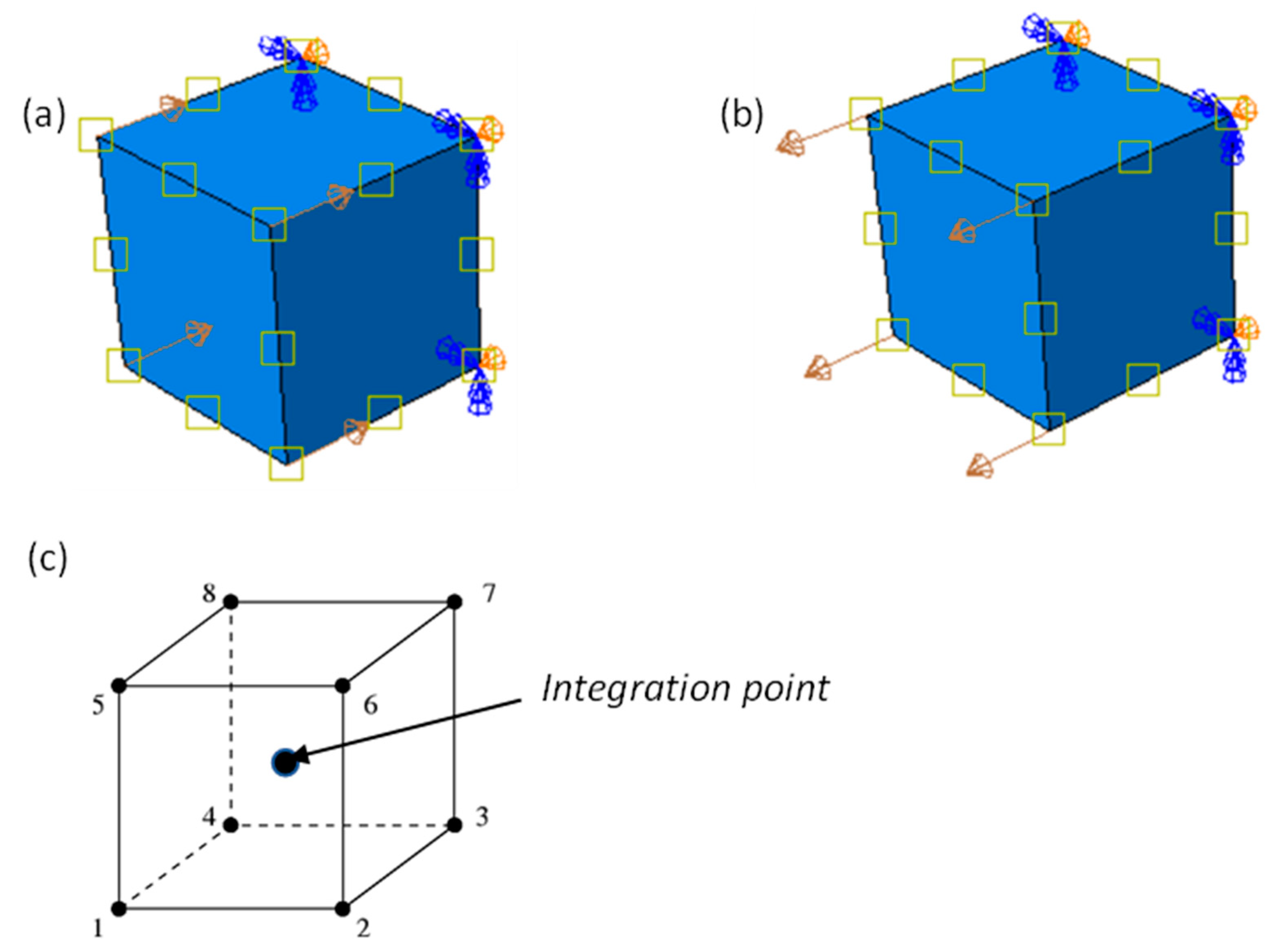
5.1. The Single Element Tests
5.2. Multiple Elements Tests
6. Conclusions
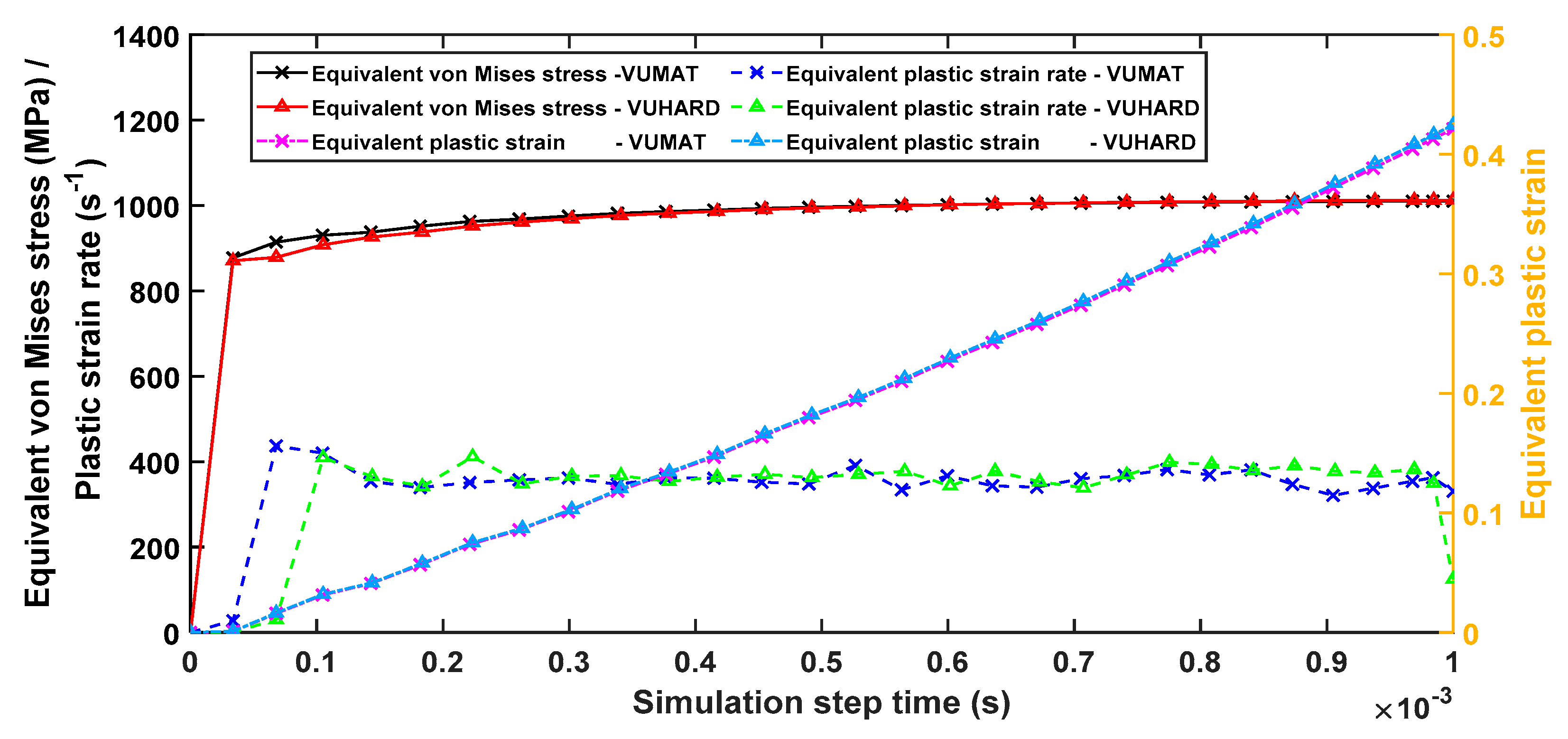
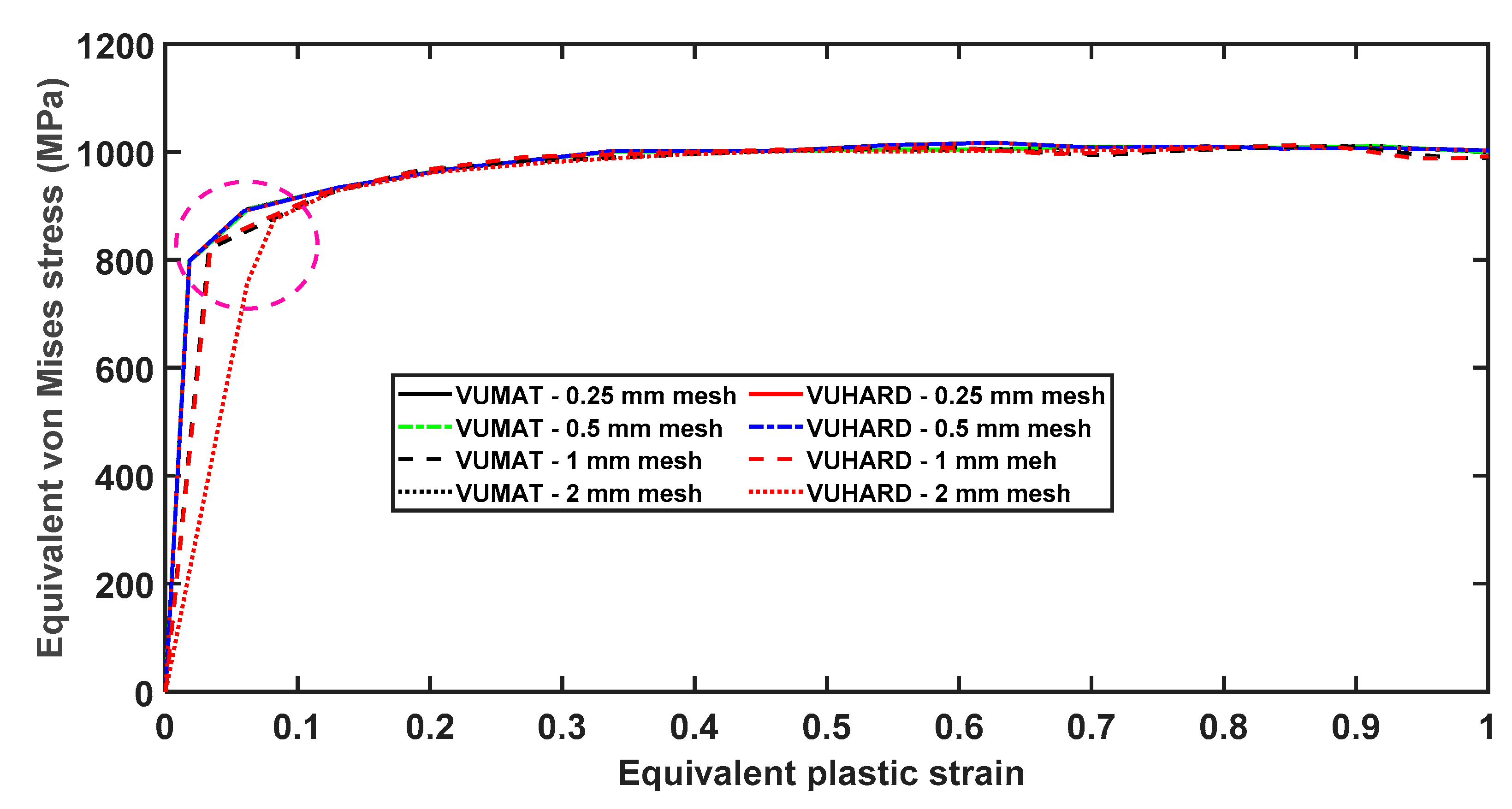
- Using single element numerical models and at a test velocity of 4 m/s, both VUMAT and VUHARD subroutines showed fairly similar values of average plastic strain rate of approximately 350 s−1.
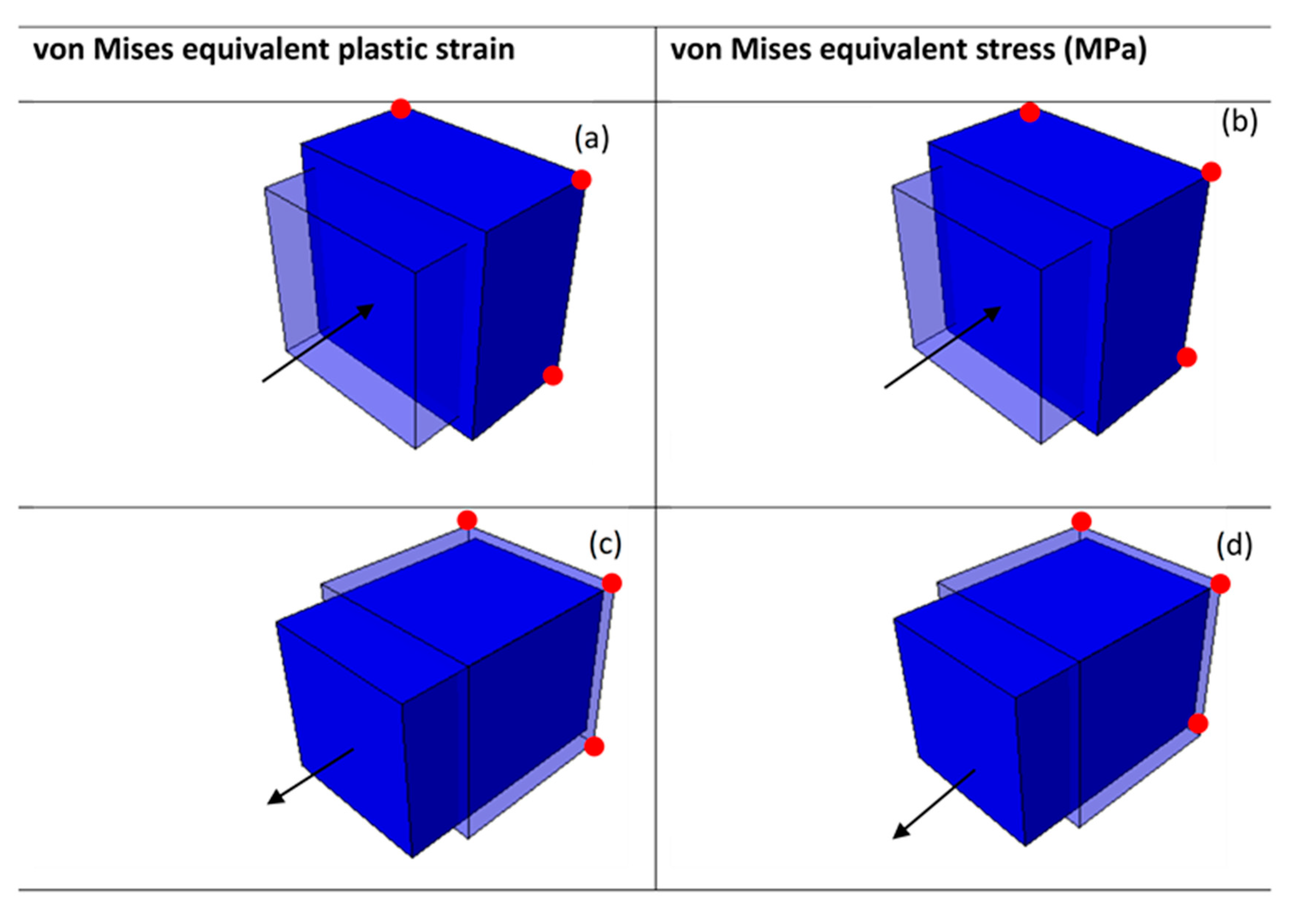
- The equivalent plastic strain and von Mises stress generated from the two subroutines for the single element numerical model also coincide for a large part of the simulation time.
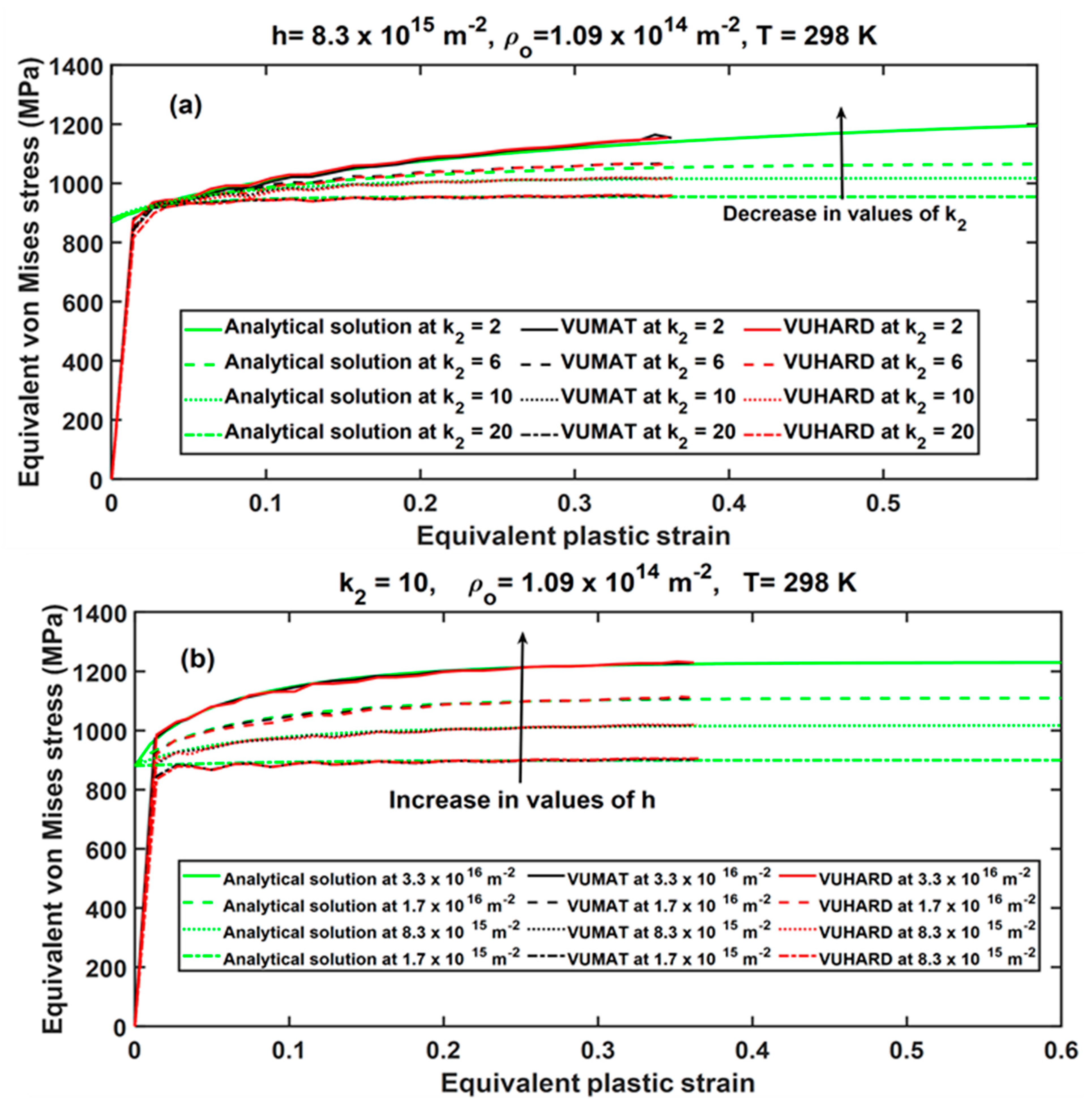
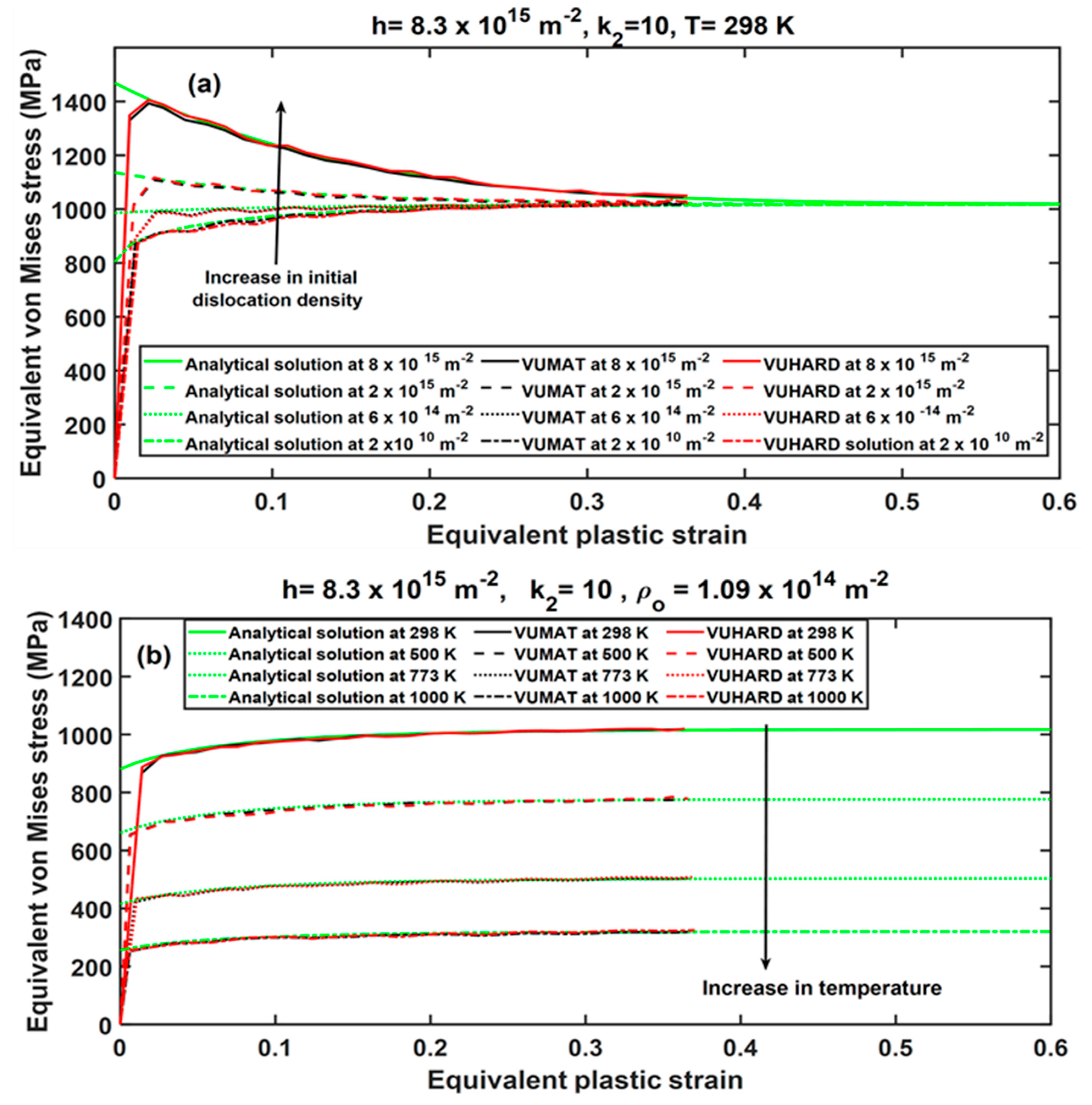
- The single element numerical models developed in this study and simulated using the developed VUMAT and VUHARD subroutines were shown to be sensitive to the critical model parameters of initial dislocation density (), test temperature (), and strain hardening and the dynamic recovery parameters and , respectively.
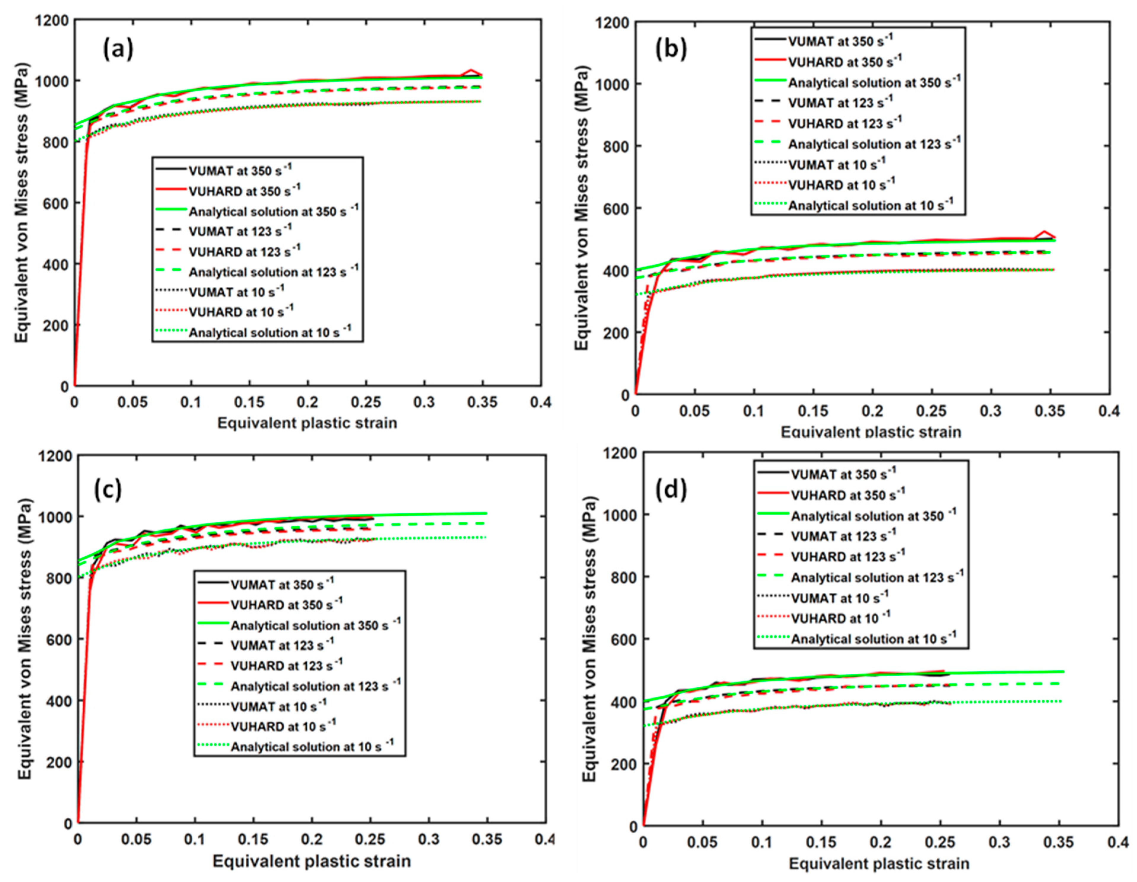
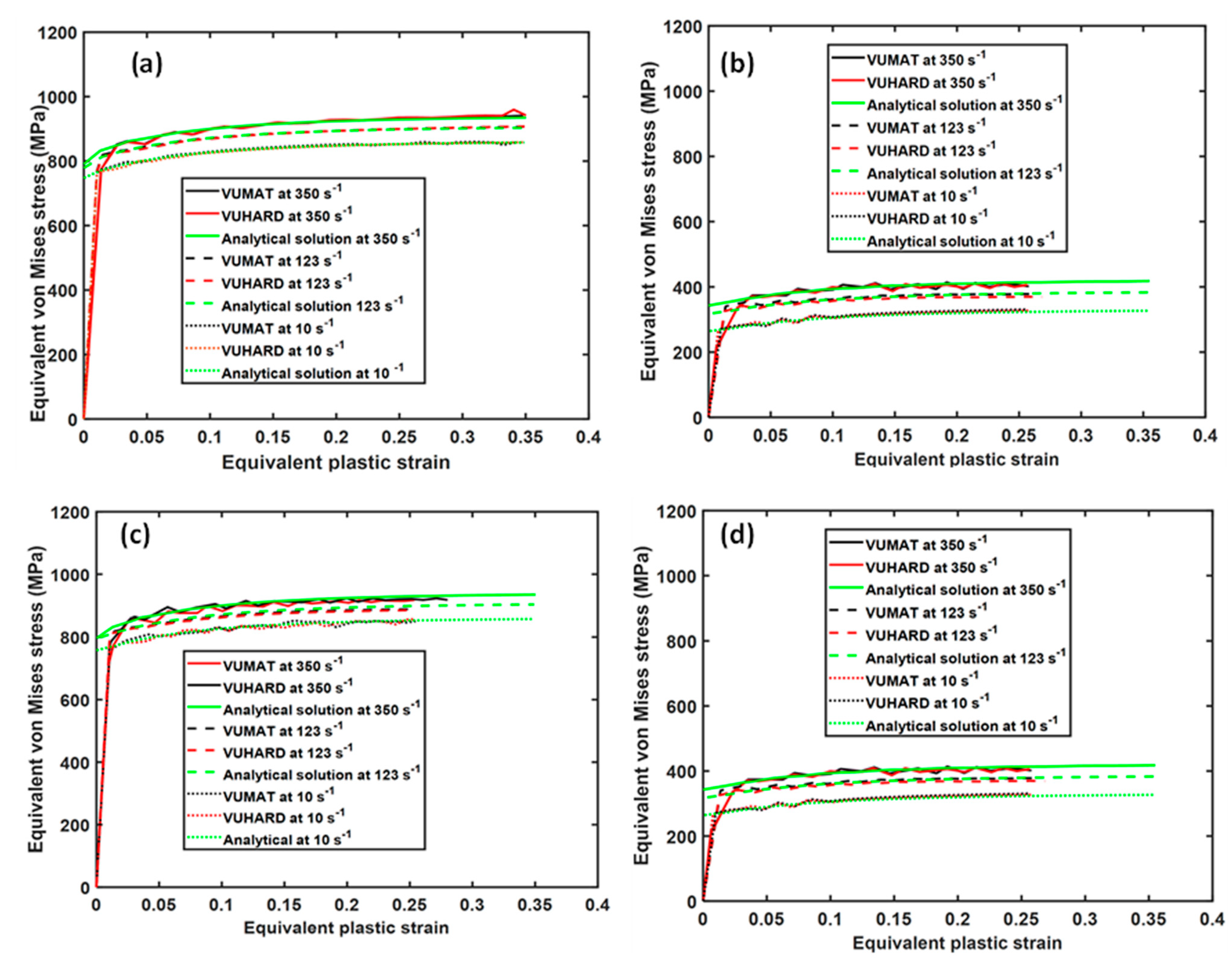
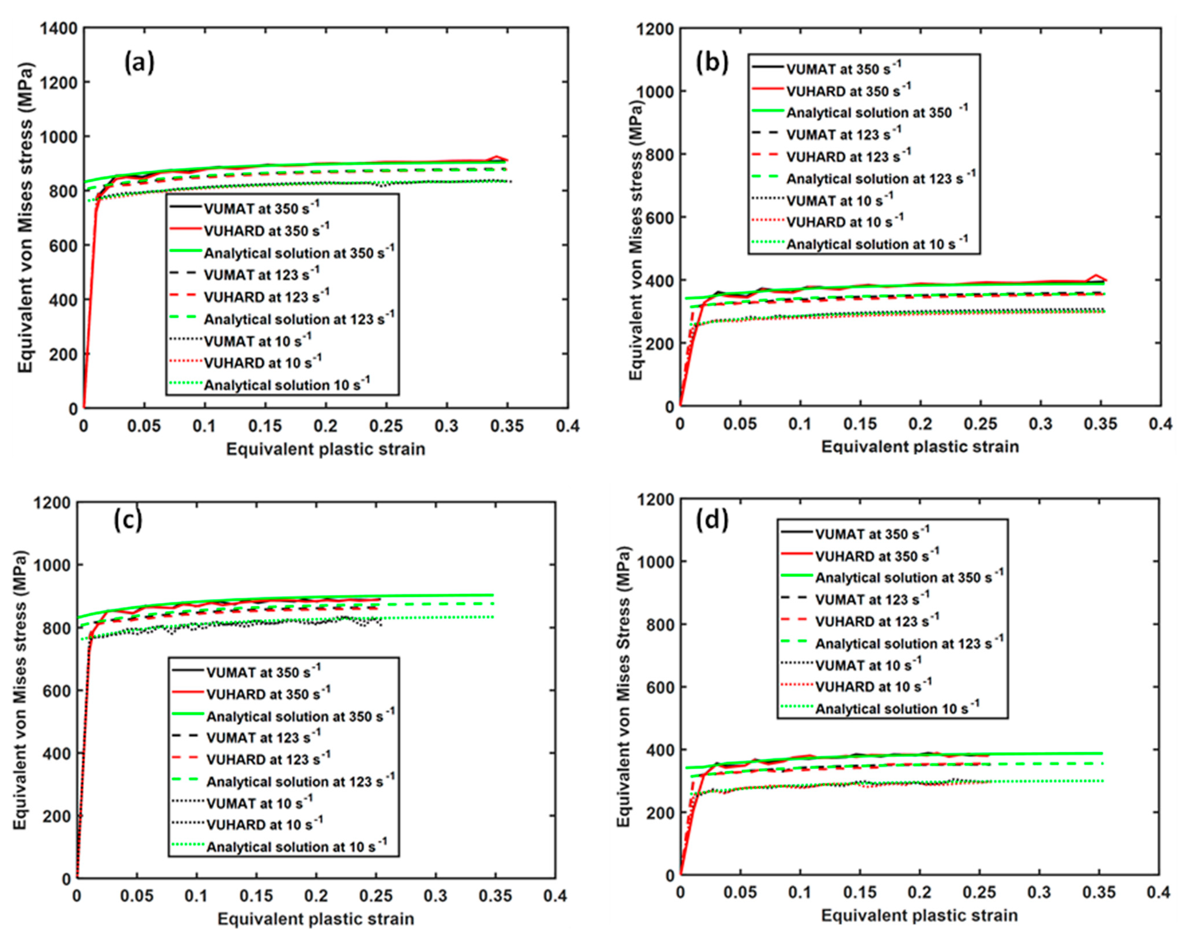
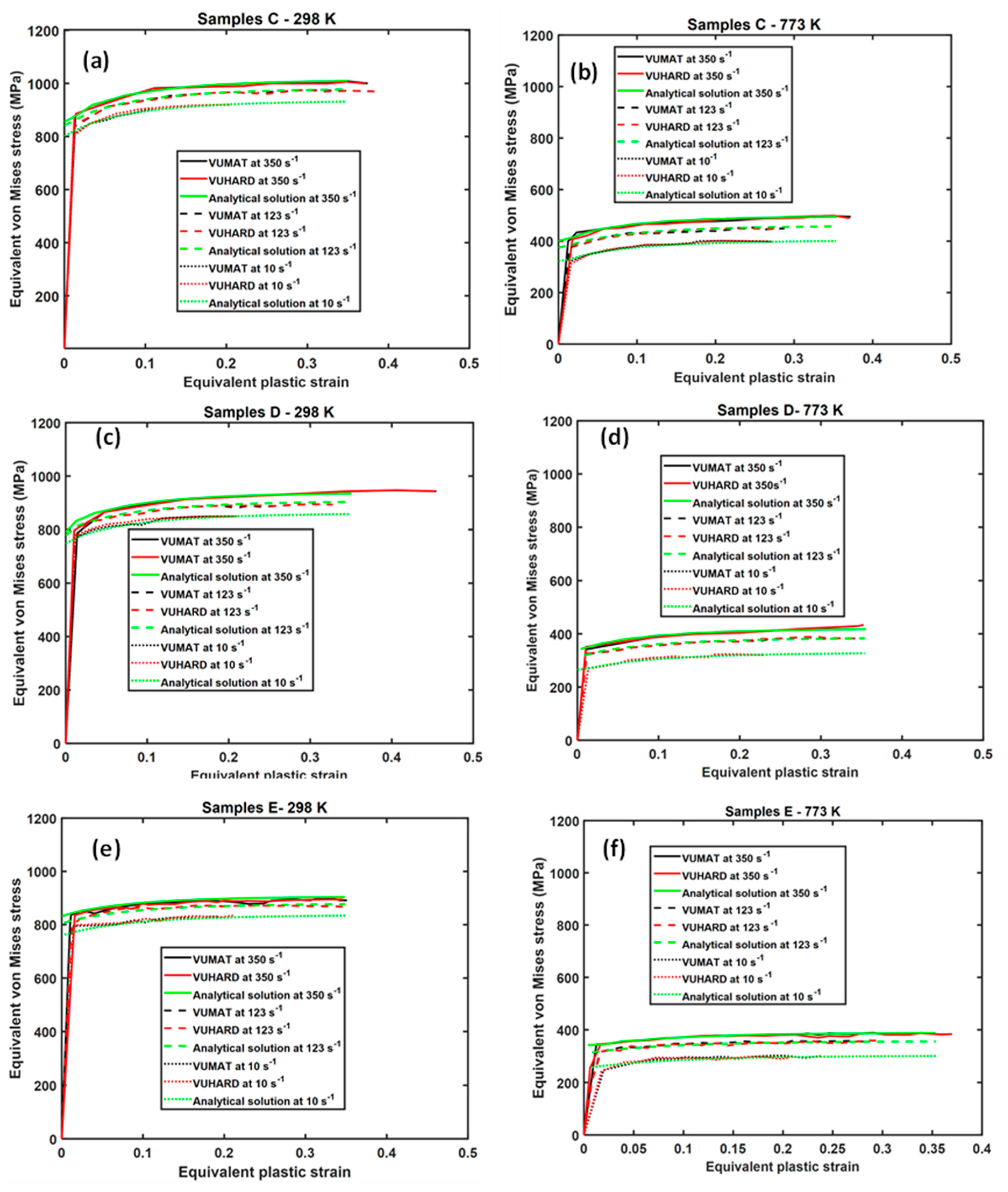
- The results of simulation of samples C, D, and E using single element numerical models based on the VUMAT and VUHARD subroutines and those derived from the analytical solutions at the same conditions of strain rate and temperature were nearly overlapping over most of plastic strain range.
- For the same simulation time, the single element numerical models showed a significant difference in the maximum equivalent plastic strain attained in the two load conditions of compression and tension, with values of about 0.35 in compression and about 0.25 in tension.
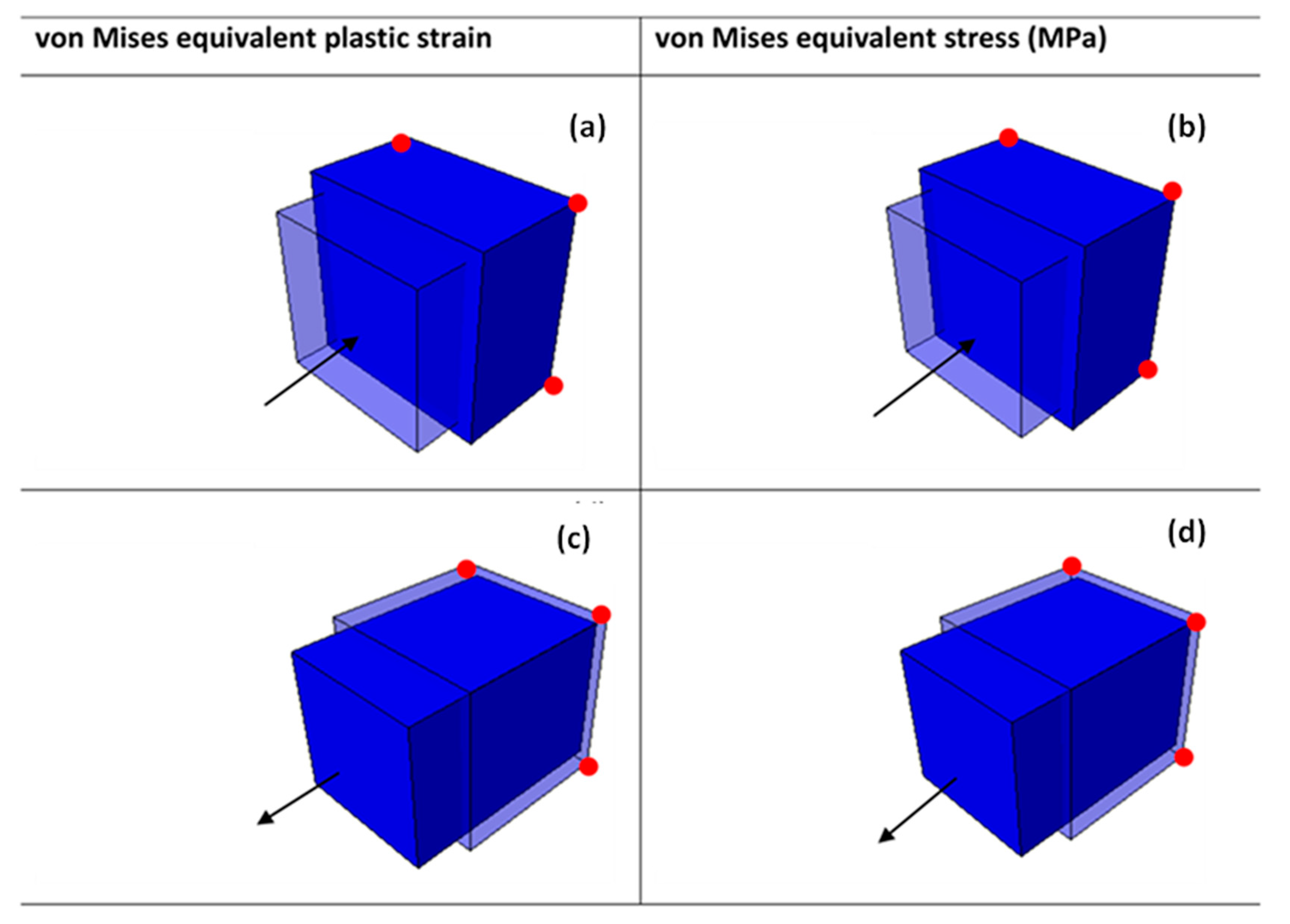
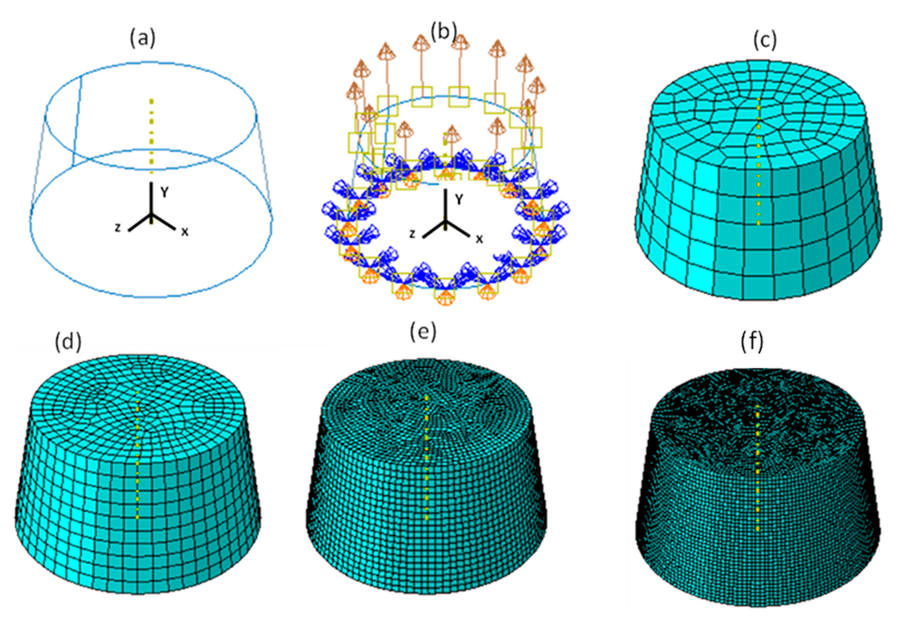
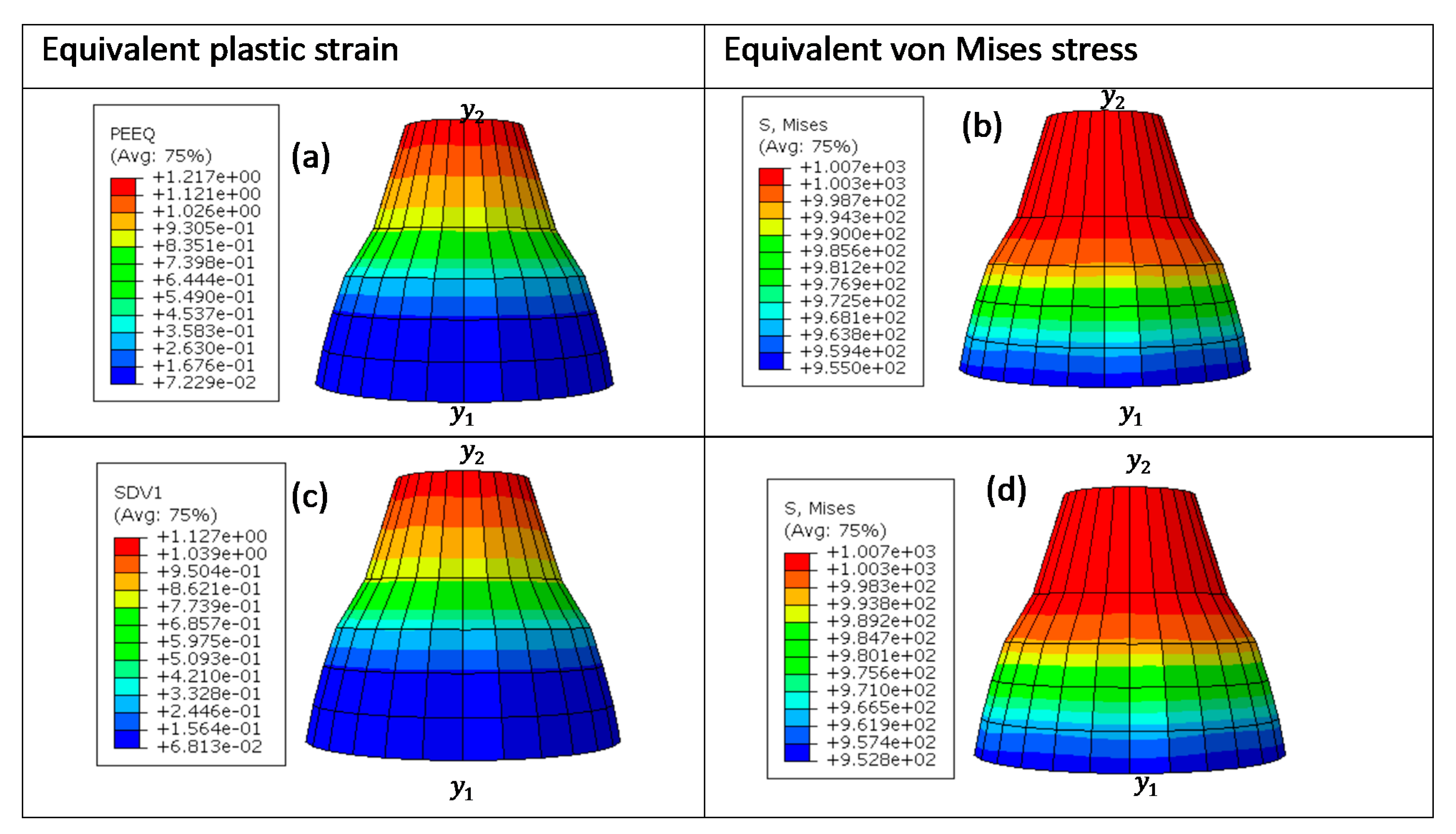
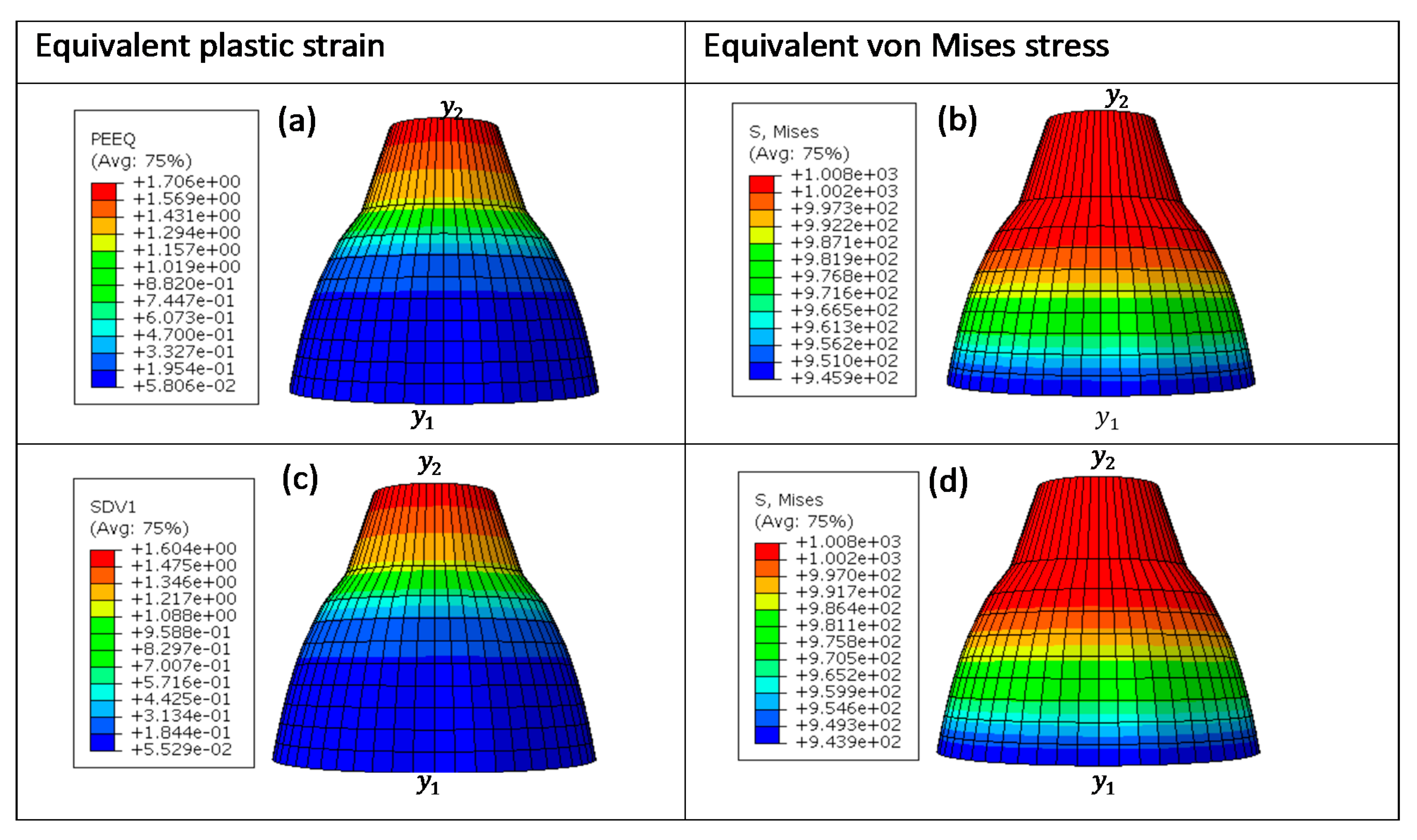
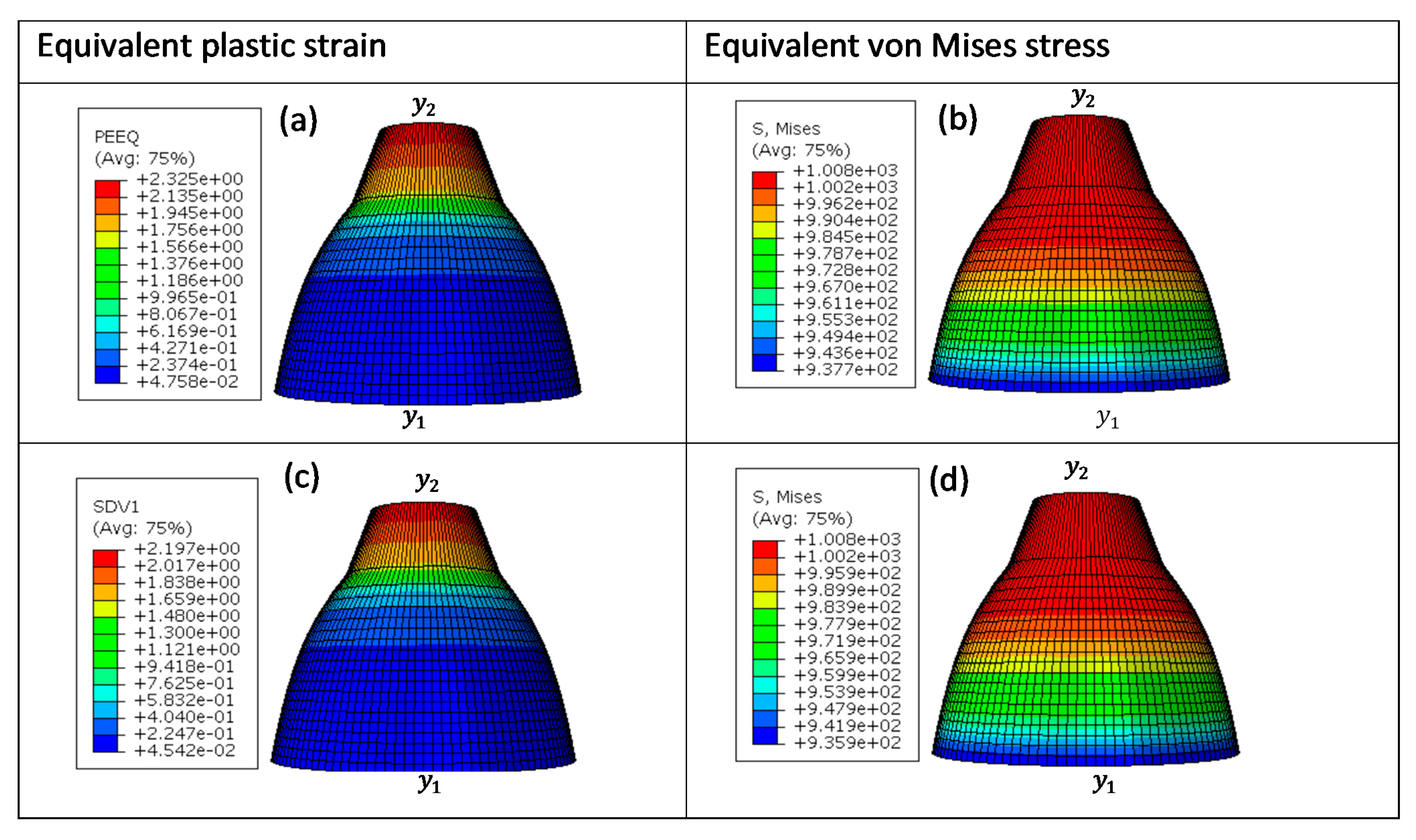
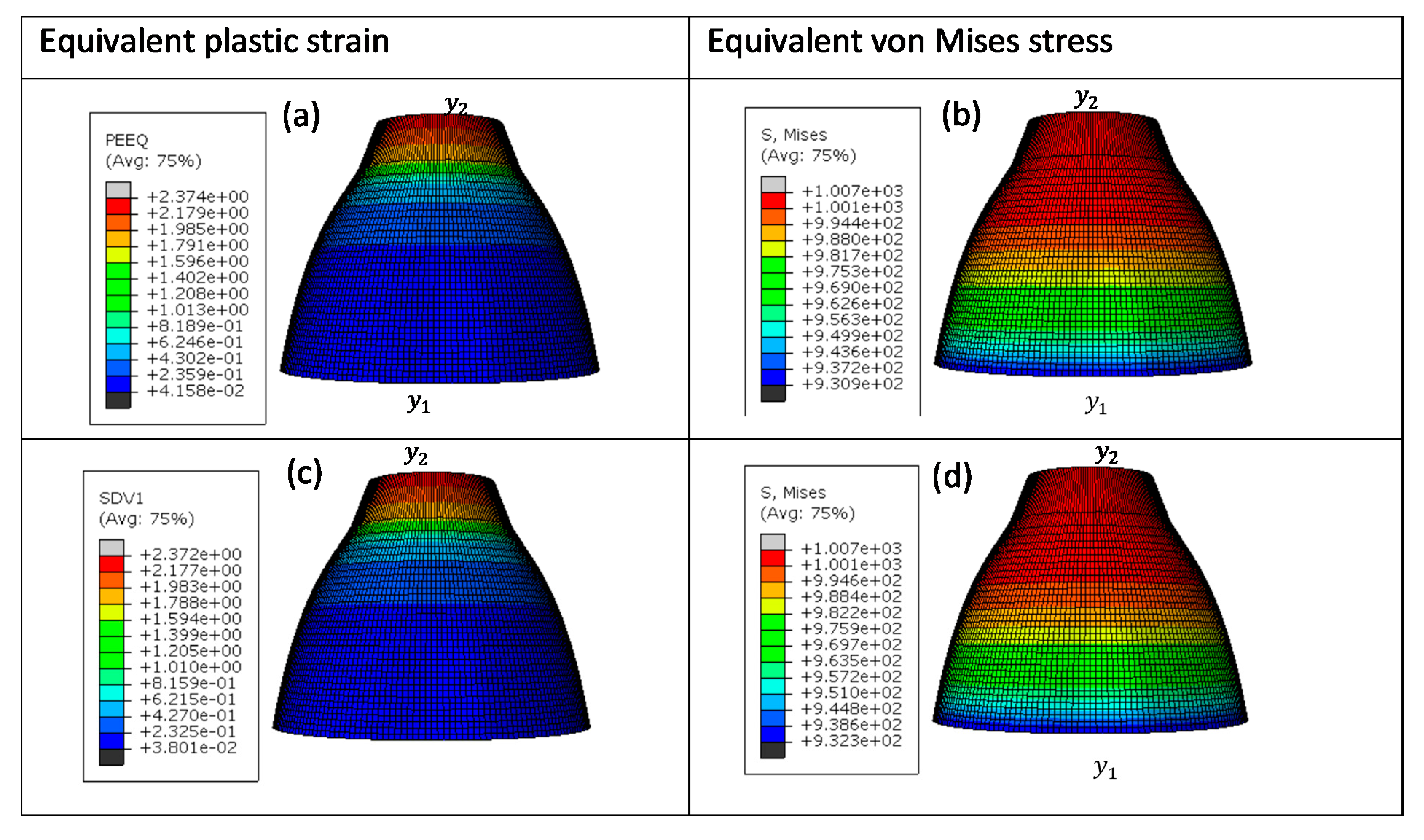
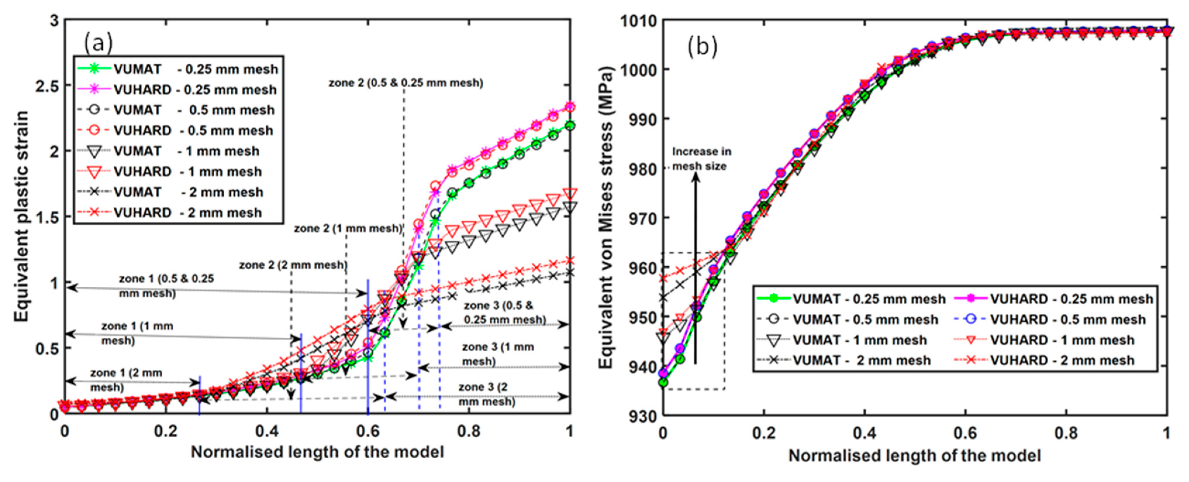
- For multiple element models with different mesh sizes, both the VUMAT and VUHARD subroutines displayed similar distributions of equivalent plastic strain and von Mises stress.
- The equivalent plastic strain and von Mises stress profiles for multiple element numerical models exhibited three typical zones which varied in range for different mesh sizes.
- The values of equivalent von Mises stress obtained in VUHARD and VUMAT subroutines varied in the first and second zones for different mesh sizes. The small variations seen in these results were attributed to the different integration schemes employed by these subroutines.
- The results obtained from both subroutines for the models with 0.25 mm and 0.5 mm mesh sizes were indistinguishable.
- Comparisons between the results obtained for the multiple element numerical modelling of samples C, D, and E and the curves obtained from analytical solutions at the same conditions of temperature and strain rate were nearly superimposed.
Supplementary Materials
Author Contributions
Funding
Institutional Review Board Statement
Informed Consent Statement
Acknowledgments
Conflicts of Interest
Appendix A. The von Mises Yield Criterion (J2) and Radial Return Algorithm
Appendix A.1. J2 Plasticity
Appendix A.2. The Radial Return Algorithms

Appendix B. The Implicit Integration Scheme to Compute for Equivalent Plastic Strain
References
- Gokuldoss, P.K.; Kolla, S.; Eckert, J. Additive manufacturing processes: Selective laser melting, electron beam melting and binder jetting—Selection guidelines. Materials 2017, 20, 672. [Google Scholar] [CrossRef] [Green Version]
- Liubov, M.; Vasilyev, B.; Kinzburskiy, V. Novel designs of turbine blades for additive manufacturing. In Proceedings of the ASME Turbo Expo: Turbine Technical Conference and Exposition, Seoul, Korea, 13–17 June 2016. [Google Scholar]
- Vignesh, M.; Ranjith, G.; Sathishkumar, M.; Manikandan, G.; Raiyalakshmi, G.; Ramanujam, R.; Arivazhagan, N. Development of biomedical implants through additive manufacturing: A review. J. Mater. Eng. Perform. 2021, 30, 4735–4744. [Google Scholar] [CrossRef]
- Zadi-Maad, A.; Rohib, R.; Irawan, A. Additive manufacturing for steels: A review. IOP Conf. Ser. Mater. Sci. Eng. 2017, 285, 012028. [Google Scholar] [CrossRef]
- Brine, C.; Shenoy, R.; Kral, M.; Buchannan, K. Precipitation behaviour of aluminum alloy 2139 fabricated using additive manufacturing. Mater.Sci. Eng. A. 2015, 648, 9–14. [Google Scholar]
- Herzog, D.; Seyda, V.; Wycisk, E.; Emmelmann, C. Additive manufacturing of metals. Acta Mater. 2016, 117, 371–392. [Google Scholar] [CrossRef]
- Aboulkhair, N.; Simonelli, M.; Parry, L.; Ashcroft, I.; Tuck, C.; Hague, R. 3D printing of aluminum alloys: Additive manufacturing of aluminum alloys using selective laser melting. Prog. Mater. Sci. 2019, 106, 100578. [Google Scholar] [CrossRef]
- Zhang, J.; Song, B.; Wei, Q.; Bourell, D.; Shi, Y. A review of selective laser melting of aluminum alloys: Processing, microstructure, property and developing trends. J. Mater. Sci. Technol. 2019, 35, 270–284. [Google Scholar] [CrossRef]
- Cotteleer, M.J. 3D Opportunity for Production. Additive Manufacturing Makes Its (Business) Case—Deloitte Review 15. 2014. Available online: https://www2.deloitte.com/us/en/insights/deloitte-review/issue-15/additive-manufacturing-business-case.html (accessed on 5 August 2021).
- Muiruri, A.; Maringa, M.; du Preez, W. Crystallographic texture analysis of as-built and heat-treated Ti6Al4V (ELI) produced by direct metal laser sintering. Crystals 2020, 10, 699. [Google Scholar] [CrossRef]
- Muiruri, A.; Maina, M.; du Preez, W.B.; Masu, L. Effects of stress relieving heat treatment on impact toughness of direct metal laser sintering (DMLS) produced Ti6Al4V (ELI) parts. JOM 2020, 72, 1175–1185. [Google Scholar] [CrossRef]
- Chae, H.; Huang, E.-W.; Woo, W.; Kang, S.; Jain, J.; An, K.; Lee, Y. Unravelling thermal history during additive manufacturing of martensitic stainless steel. J. Alloy. Compd. 2021, 857, 157555. [Google Scholar] [CrossRef] [PubMed]
- Eshawish, N.; Malinov, S.; Sha, W.; Walls, P. Microstructure, and mechanical properties of Ti6Al4V manufactured by selective laser melting after stress relieving, hot isostatic pressing treatment and post-heat treatment. J. Mater. Eng. Perform. 2021, 30, 5290–5296. [Google Scholar] [CrossRef]
- Omonyi, P.; Akinlabi, E.; Mahamood, M. Heat treatments of Ti6Al4V alloys for industrial applications: An overview. IOP Conf. Ser. Mater. Sci. Eng. 2021, 1107, 012094. [Google Scholar] [CrossRef]
- Vrancken, B.; Thijs, L.; Kruth, J.P.; Humbeeck, J.V. Heat treatment of Ti6Al4V produced by selective laser melting: Microstructure and mechanical properties. J. Alloy. Compd. 2012, 541, 177–185. [Google Scholar] [CrossRef] [Green Version]
- Dieter, E.G. Mechanical Metallurgy: Material Science and Engineering Series, 3rd ed.; McGraw-Hill: New York, NY, USA, 1986; pp. 103–184. [Google Scholar]
- Armendáriz, I.; Millán, J.; Encinas, J.; Olarrea, J. Strategies for dynamic failure analysis on aerospace structures. In Handbook of Materials Failure Analysis: With Case Studies from the Aerospace and Automotive Industries; Salam, A., Makhlouf, H., Mahmood, A., Eds.; Elsevier Ltd.: Amsterdam, The Netherlands, 2016; pp. 29–55. [Google Scholar]
- Sun, Y.; Weidong, Z.; Yuanfei, H.; Xiong, M.; Yongqing, Z.; Ping, G.; Wang, G.; Dargusch, S. Determination of the influence of processing parameters on the mechanical properties of the Ti6Al4V alloy using an artificial neural network. Comput. Mater. Sci. 2012, 60, 239–244. [Google Scholar] [CrossRef]
- Jaimie, S.; Tiley, M.S. Modelling of Microstructure Property Relationships in Ti6Al4V. Ph.D. Thesis, Graduate School of the Ohio State University, Columbus, OH, USA, 2002. [Google Scholar]
- Song, X.; Feih, S.; Zhai, W.; Sun, C.-N.; Feng, L.; Maiti, R.; Wei, J.; Yang, Y.; Oancea, V.; Brandt, R.; et al. Advances in additive manufacturing process simulation: Residual stresses and distortion predictions in complex metallic components. Mater. Des. 2020, 193, 108779. [Google Scholar] [CrossRef]
- Marques, B.; Andrade, C.; Neto, D.; Oliveira, M.; Alves, J.; Menezes, L. Numerical analysis of residual stresses in parts produced by selective laser melting process. Procedia Manuf. 2020, 47, 1170–1177. [Google Scholar] [CrossRef]
- Chen, Y.; Chen, H.; Chen, J.-Q.; Xiong, J.; Wu, Y.; Dong, S.-Y. Numerical and experimental investigation on thermal behaviour and microstructure during selective laser melting of high strength steel. J. Manuf. Process. 2020, 57, 533–542. [Google Scholar] [CrossRef]
- Zinoviev, A.; Zinovieva, O.; Ploshikhin, V.; Romanova, V.; Balokhonov, R. Evolution of grain structure during laser additive manufacturing. Simulation by a cellular automata method. Mater. Des. 2016, 106, 321–329. [Google Scholar] [CrossRef]
- Yang, J.; Hanchen, Y.; Yang, H.; Fanzhi, L.; Wang, Z.; Zeng, X. Prediction of microstructure in selective laser melted Ti6Al4V alloy by cellular automation. J. Alloy. Compd. 2018, 748, 281–290. [Google Scholar] [CrossRef]
- Nasiri, S.; Khosravani, R. Machine learning in predicting mechanical behaviour of additively manufactured parts. J. Mater. Res. Technol. 2021, 14, 1137–1153. [Google Scholar] [CrossRef]
- Wan, H.; Chen, G.; Li, C.; Qi, X.; Zhang, G. Data-driven evaluation of fatigue performance of additive manufactured parts using miniature specimens. J. Mater. Sci. Technol. 2019, 25, 1137–1146. [Google Scholar] [CrossRef]
- ABAQUS Documentation. 2020. Available online: https://help.3ds.com/2020/English/DSSIMULIA_Established/SIMULIA_Established_FrontmatterMap/HelpViewerDS.aspx?version=2020&prod=DSSIMULIA_Established&lang=English&path=SIMULIA_Established_FrontmatterMap%2fsim-r-DSDocAbaqus.htm&ContextScope=all (accessed on 12 November 2020).
- Muiruri, A.; Maringa, M.; du Preez, W. High strain rate properties of various forms of Ti6Al4V (ELI) produced by direct metal laser sintering. Appl. Sci. 2021, 11, 8005. [Google Scholar] [CrossRef]
- Muiruri, A.; Maringa, M.; du Preez, W. Validation of a microstructure-based model for predicting the high strain rate flow properties of various forms of additively manufactured Ti6Al4V (ELI) alloy. Metals 2021, 11, 1628. [Google Scholar] [CrossRef]
- Muiruri, A.; Maringa, M.; du Preez, W. Evaluation of dislocation densities in various microstructures of additively manufactured Ti6Al4V (ELI) by the method of x-ray diffraction. Materials 2020, 13, 5355. [Google Scholar] [CrossRef]
- Tvergaard, V.; Needleman, A. Analysis of the cup-cone fracture in a round tensile bar. Acta Metall. 1984, 32, 157–169. [Google Scholar] [CrossRef]
- Ming, L.; Pantalé, O. An efficient and robust VUMAT implementation of elastoplastic constitutive laws in ABAQUS/explicit finite element code. Mech. Ind. 2018, 19, 308. [Google Scholar] [CrossRef] [Green Version]
- Stouffer, D.C.; Dame, L.T. Inelastic Deformation of Metals: Models, Mechanical Properties and Metallurgy; John Wiley & Sons Inc.: Hoboken, NJ, USA, 1996; pp. 120–145. [Google Scholar]
- Fischer, C.; Antony, C. Introduction to Contact Mechanics, 2nd ed.; Springer Science Business Media: New York, NY, USA, 2007; p. 36. [Google Scholar]
- Feng, K.; Shi, Z.-C. Static elasticity. In Mathematical Theory of Elastic Structures; Springer: Berlin/Heidelberg, Germany, 1996; pp. 89–138. [Google Scholar]
- Lubliner, J. Plasticity Theory; Macmillan Publishing Company: New York, NY, USA, 1990; pp. 69–82. [Google Scholar]
- Wilkins, M.L. Calculations of elastic-plastic flow. In Methods in Computations Physics; Alder, B., Ed.; Academic Press: Millbrae, CA, USA, 1963; Volume 3, pp. 211–263. [Google Scholar]


| Sample Type | Average Grain Size | Average Initial Dislocation Density |
|---|---|---|
| C | 2.5 | 5.73 × 10¹⁴ |
| D | 6.0 | 5.09 × 10¹⁴ |
| E | 9.0 | 7.00 × 10¹⁴ |
| Prescribed Parameters | Value and Units | Fitted Parameters | Values and Units |
|---|---|---|---|
| Boltzmann constant ) | 1.38 × 10⁻²³ m2kgs−2 k−1 | 1063.2 MPa | |
| Shear modulus | 0.25 | ||
| Burgers vector (b) | 8.3 × 10¹⁵ m−2 | ||
| Reference strain rate | 107 s−1 | 10 | |
| Hall–Petch constant () | ζ | (MPa) | |
| P | 1 | Samples C | 207 |
| Q | 2 | Samples D | 210 |
| Taylor factor () | 3 | Samples E | 210 |
| 0.2 | |||
| Samples C | 0.00032 | ||
| Samples D | 0.00030 | ||
| Samples E | 0.00020 |
| Variables | VUHARD | ABAQUS | VUMAT | ABAQUS |
|---|---|---|---|---|
| Elastic modulus | - | - | Props (1) | |
| Poisson’s ratio | - | - | Props (2) | |
| K/b3 | Kb3 | Props (1) | Kb3 | Props (3) |
| goi | Goi | Props (2) | goi | Props (4) |
| ddeqps0 | Props (3) | ddeqps0 | Props (5) | |
| Theta | Props (4) | theta | Props (6) | |
| p | P | Props (5) | p | Props (7) |
| q | Q | Props (6) | q | Props (8) |
| e0 | Props (7) | e0 | Props (9) | |
| h | H | Props (8) | h | Props (10) |
| k2 | k2 | Props (9) | k2 | Props (11) |
| α × b × M | Abm | Props (10) | abm | Props (12) |
| Khp | Props (11) | Khp | Props (13) | |
| Alpha | Props (12) | alpha | Props (14) | |
| Ala | Props (13) | ala | Props (15) | |
| t | T | Props (14) | t | Props (16) |
| U0 | U0 | Props (15) | U0 | Props (17) |
| D | D | Props (16) | D | Props (18) |
| T0 | T0 | Props (17) | T0 | Props (19) |
| Subroutine | VUHARD | VUMAT | ||
|---|---|---|---|---|
| Mesh Size (mm) | Time (s) | Increments | Time (s) | Increments |
| 2 | 6.3 | 92 | 9.2 | 96 |
| 1 | 59.3 | 200 | 63.2 | 219 |
| 0.5 | 177.2 | 447 | 396.6 | 629 |
| 0.25 | 1676 | 900 | 1876 | 1037 |
Publisher’s Note: MDPI stays neutral with regard to jurisdictional claims in published maps and institutional affiliations. |
© 2022 by the authors. Licensee MDPI, Basel, Switzerland. This article is an open access article distributed under the terms and conditions of the Creative Commons Attribution (CC BY) license (https://creativecommons.org/licenses/by/4.0/).
Share and Cite
Muiruri, A.; Maringa, M.; du Preez, W. Development of VUMAT and VUHARD Subroutines for Simulating the Dynamic Mechanical Properties of Additively Manufactured Parts. Materials 2022, 15, 372. https://doi.org/10.3390/ma15010372
Muiruri A, Maringa M, du Preez W. Development of VUMAT and VUHARD Subroutines for Simulating the Dynamic Mechanical Properties of Additively Manufactured Parts. Materials. 2022; 15(1):372. https://doi.org/10.3390/ma15010372
Chicago/Turabian StyleMuiruri, Amos, Maina Maringa, and Willie du Preez. 2022. "Development of VUMAT and VUHARD Subroutines for Simulating the Dynamic Mechanical Properties of Additively Manufactured Parts" Materials 15, no. 1: 372. https://doi.org/10.3390/ma15010372