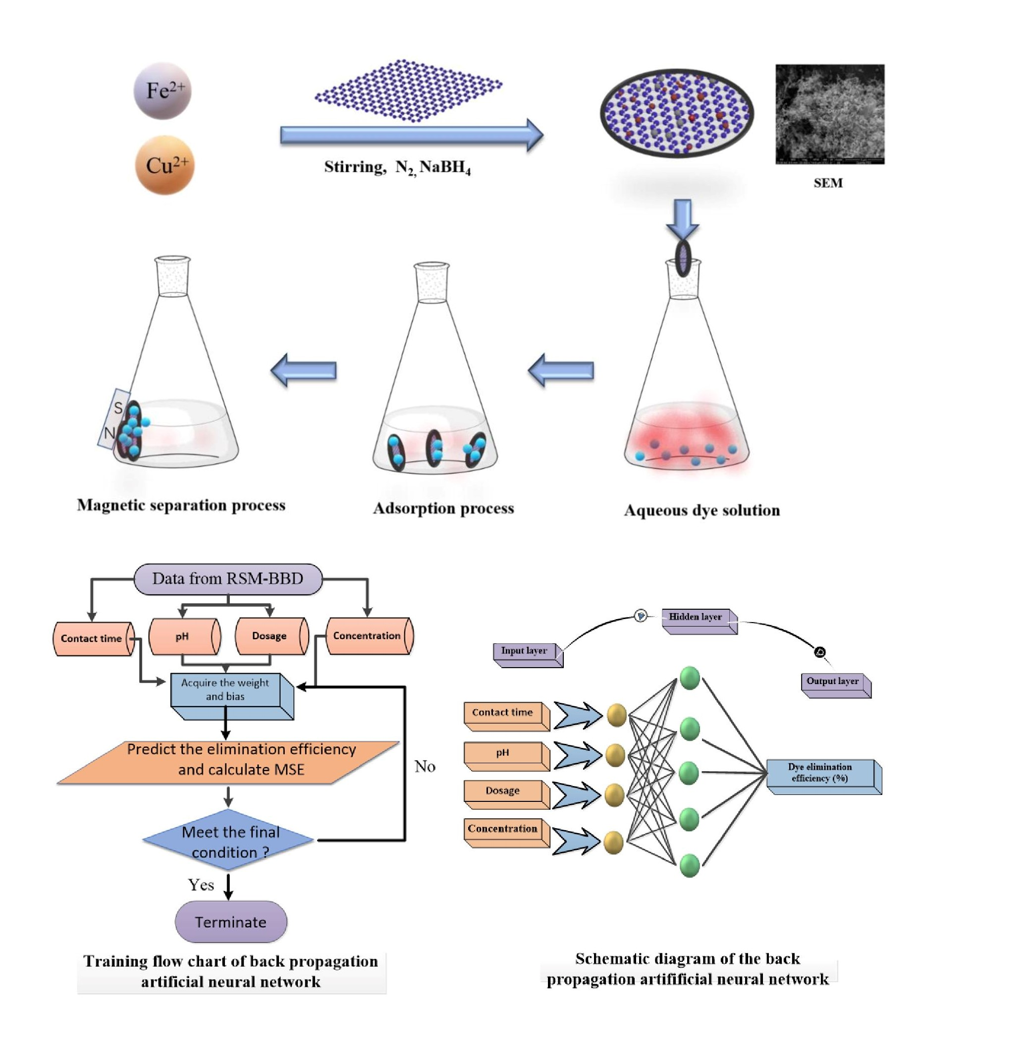
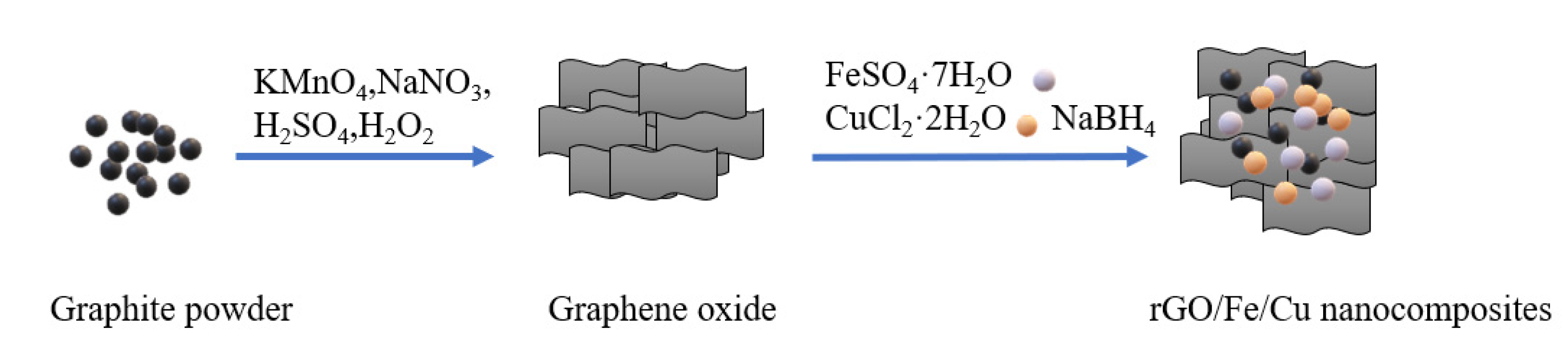
Figure 1.
Schematic of rGO/Fe/Cu nanocomposite synthesis.
Figure 1.
Schematic of rGO/Fe/Cu nanocomposite synthesis.
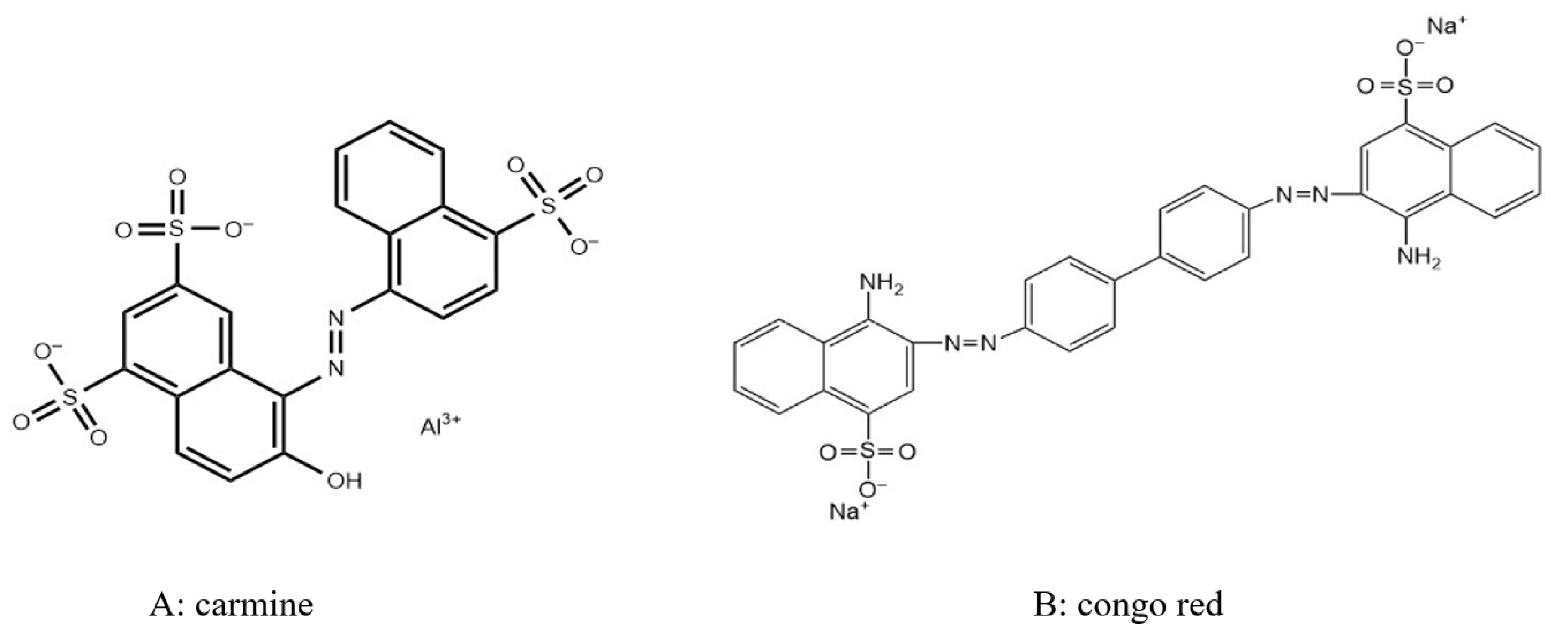
Figure 2.
Structure of carmine (A) and Congo red (B).
Figure 2.
Structure of carmine (A) and Congo red (B).
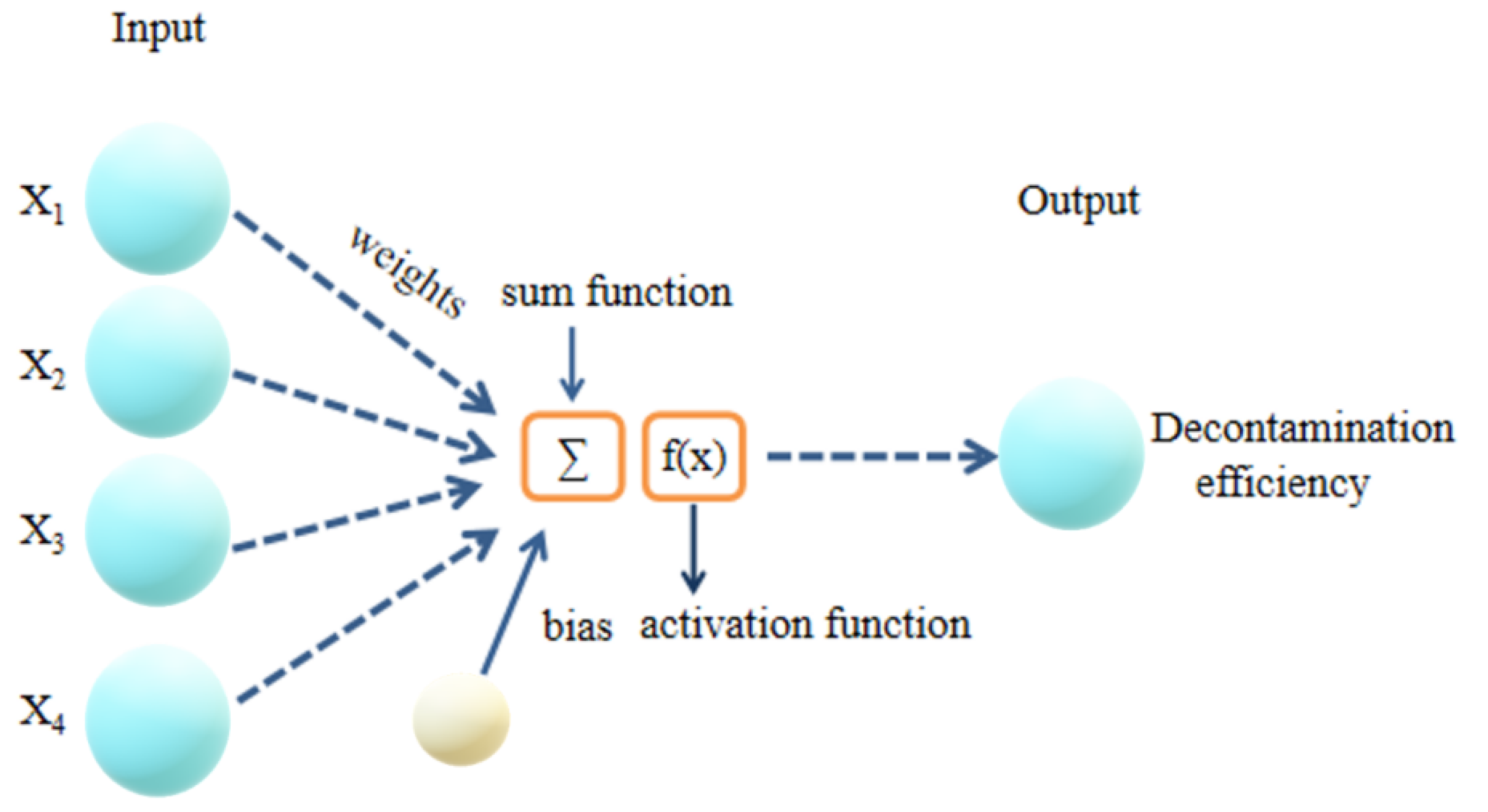
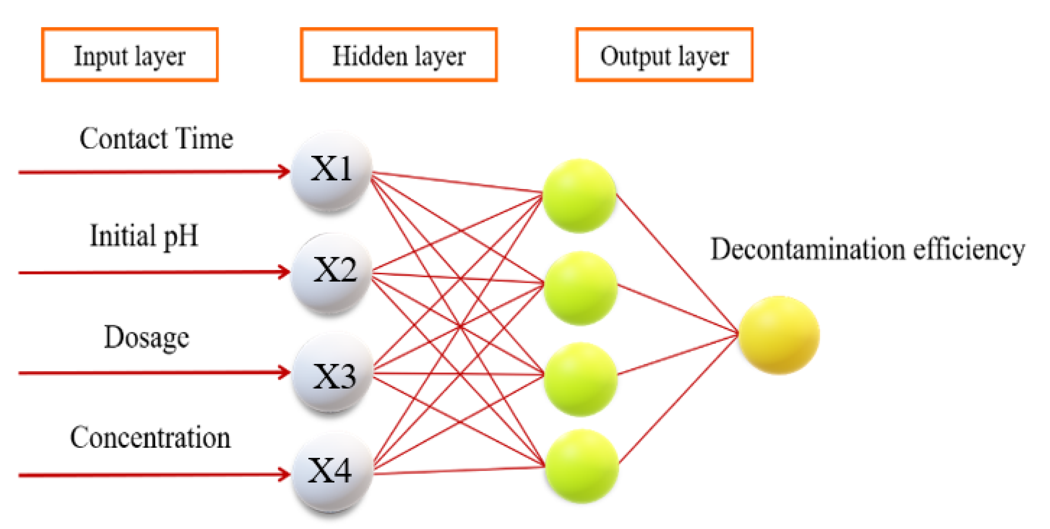
Figure 3.
The schematic diagram for the artificial neuron model.
Figure 3.
The schematic diagram for the artificial neuron model.
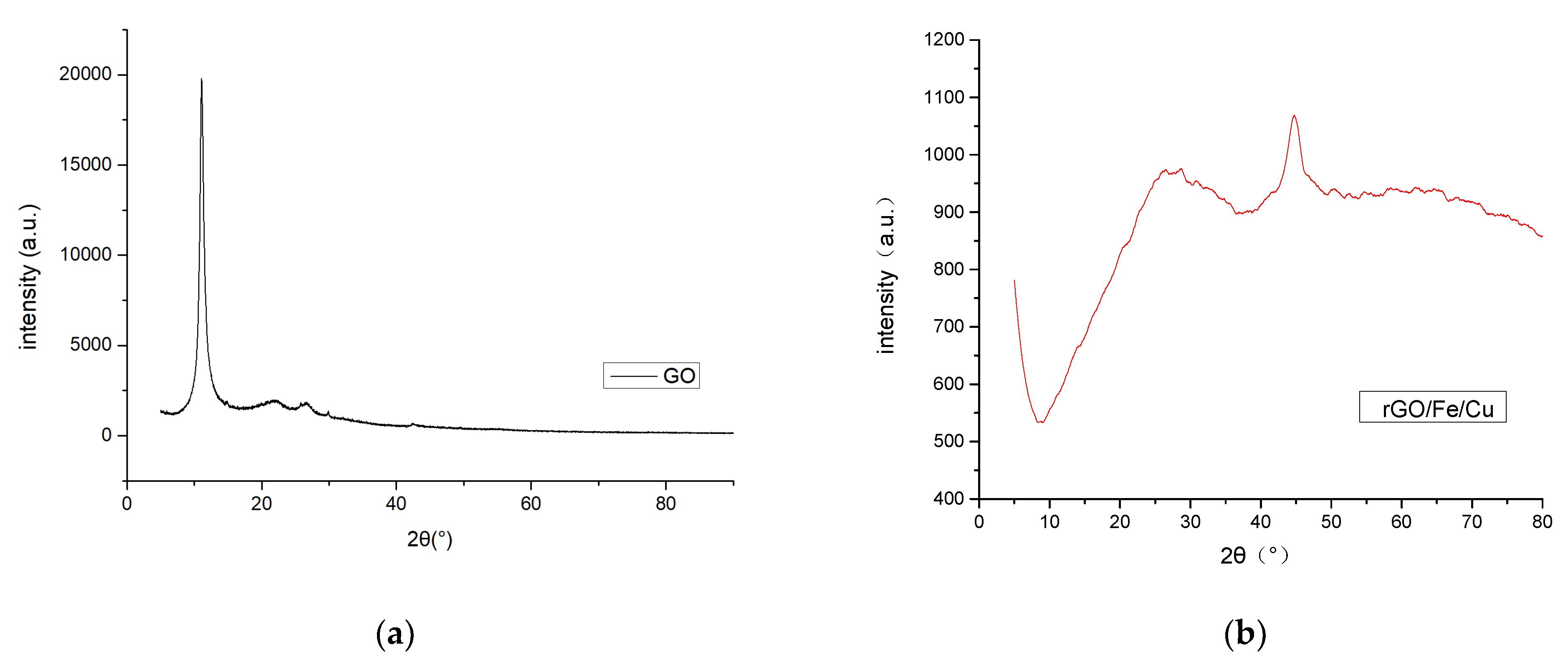
Figure 4.
X-ray diffraction (XRD) patterns of (a) GO and (b) rGO/Fe/Cu nanocompounds.
Figure 4.
X-ray diffraction (XRD) patterns of (a) GO and (b) rGO/Fe/Cu nanocompounds.
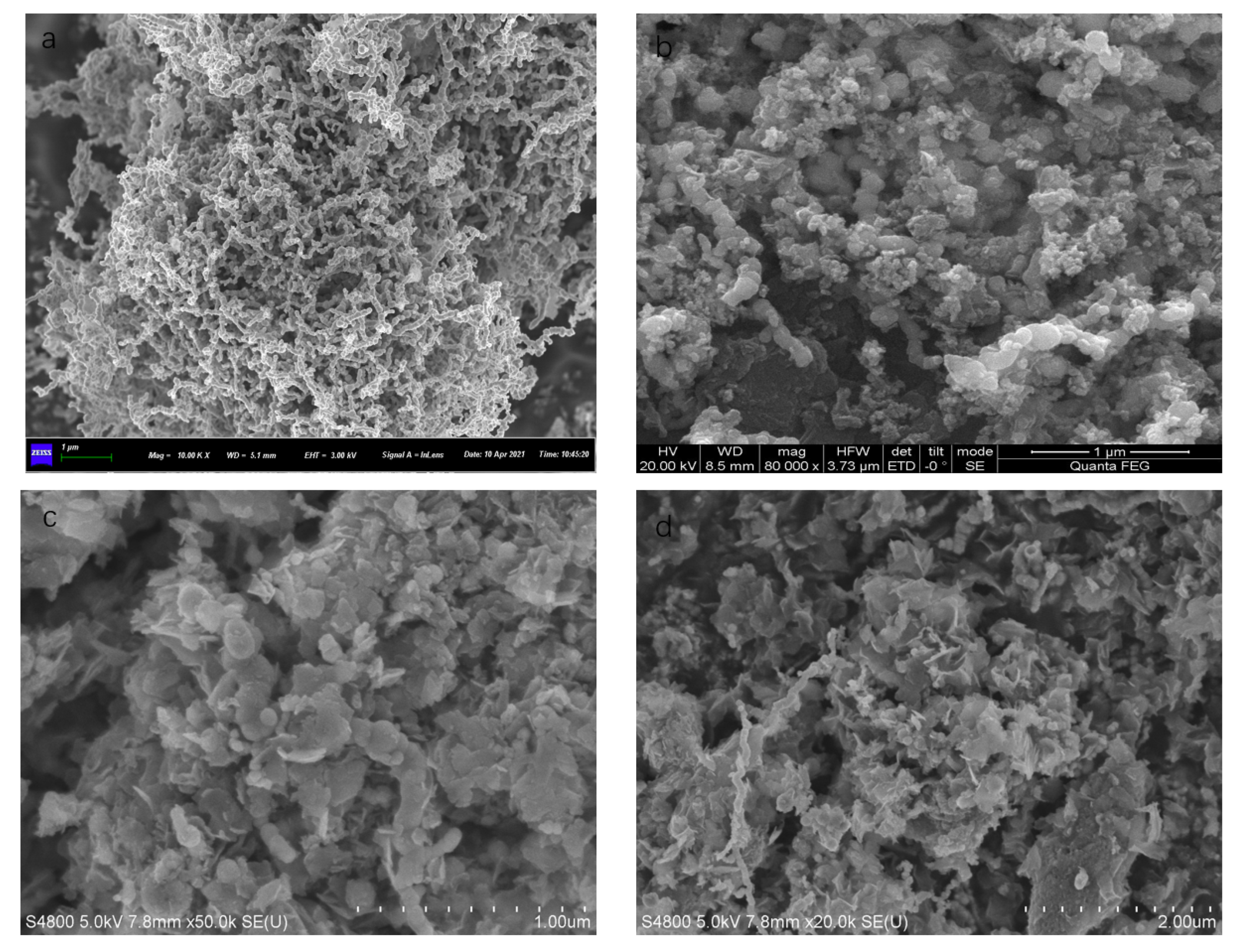
Figure 5.
SEM images of Fe/Cu (a) and rGO/Fe/Cu (b) and the rGO/Fe/Cu at 1 um (c) and 2 um (d) after the experiment.
Figure 5.
SEM images of Fe/Cu (a) and rGO/Fe/Cu (b) and the rGO/Fe/Cu at 1 um (c) and 2 um (d) after the experiment.
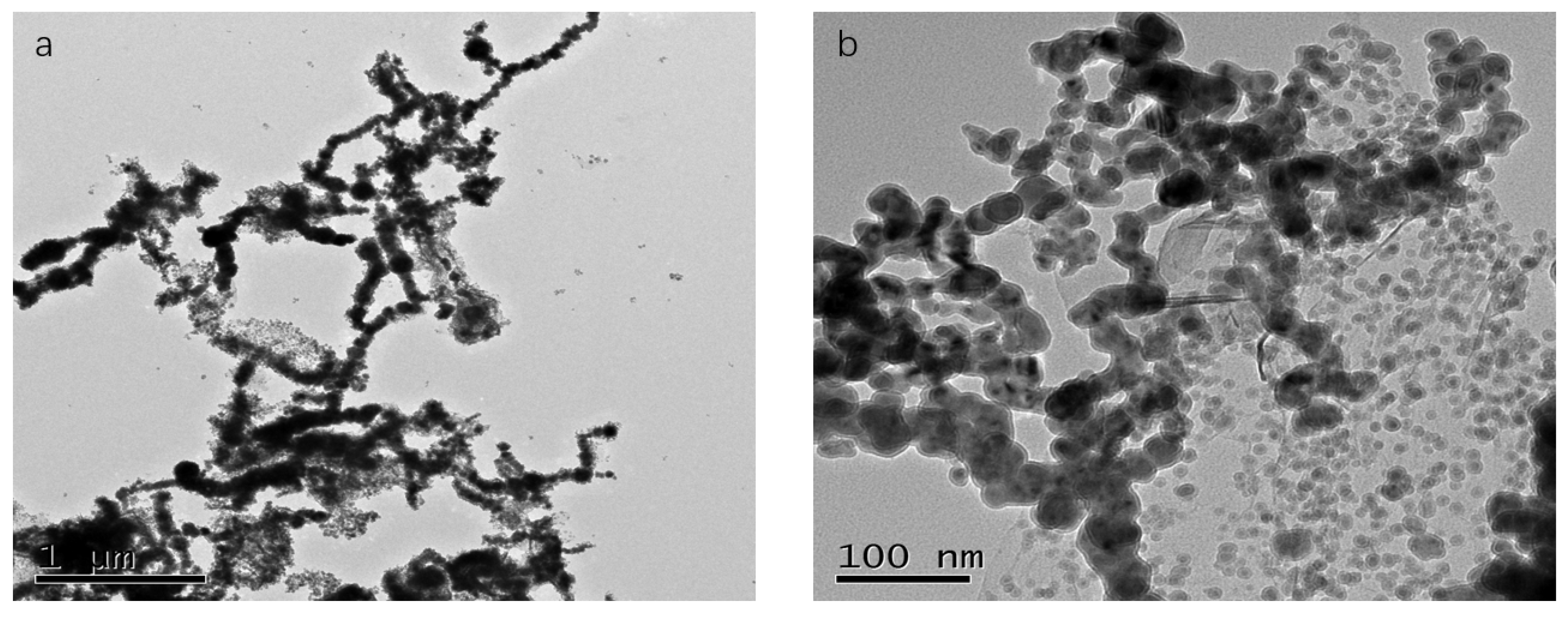
Figure 6.
TEM images of Fe/Cu (a) and rGO/Fe/Cu (b).
Figure 6.
TEM images of Fe/Cu (a) and rGO/Fe/Cu (b).
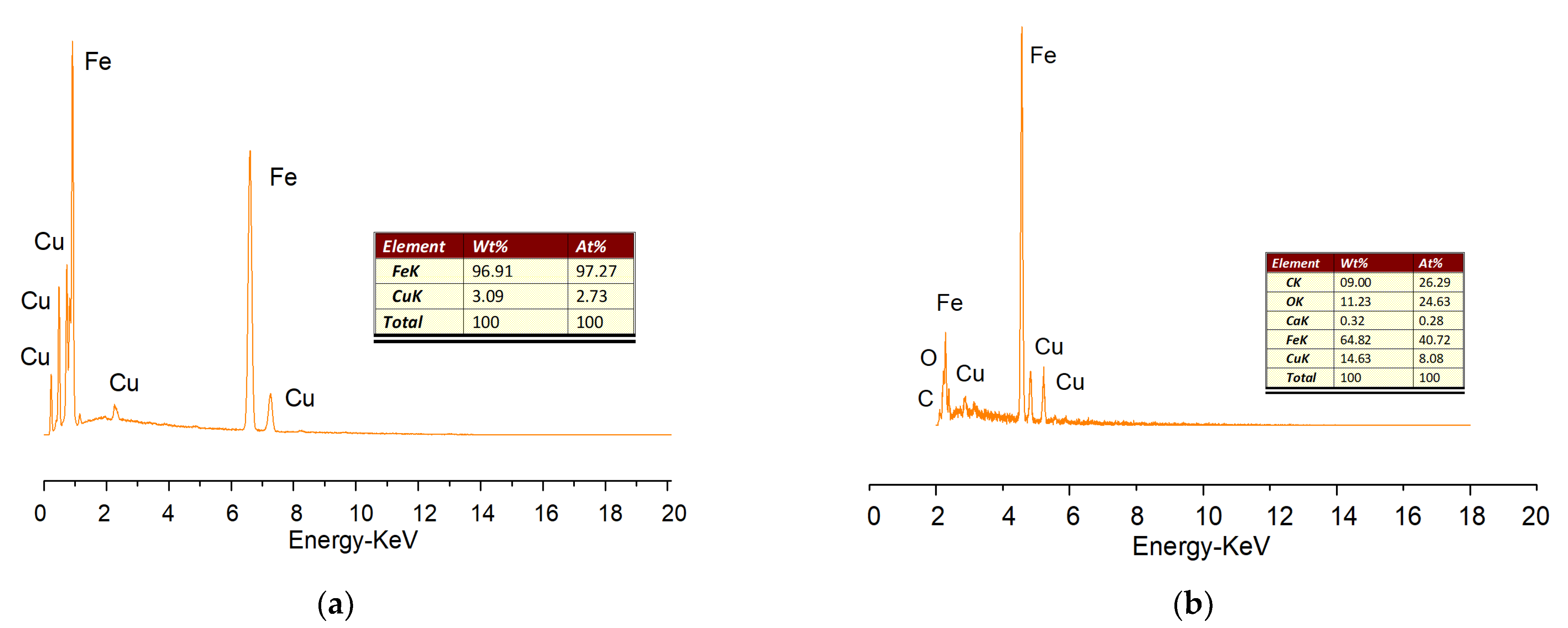
Figure 7.
EDS spectra of the (a) Fe/Cu nanoparticles and (b) rGO/Fe/Cu nanocompounds.
Figure 7.
EDS spectra of the (a) Fe/Cu nanoparticles and (b) rGO/Fe/Cu nanocompounds.
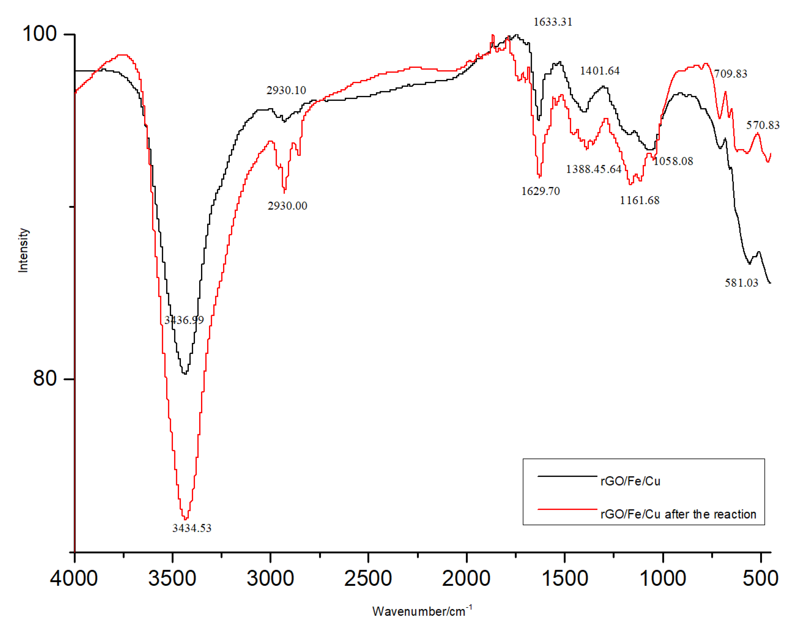
Figure 8.
FTIR spectra of rGO/Fe/Cu nanocompounds before and after the reaction.
Figure 8.
FTIR spectra of rGO/Fe/Cu nanocompounds before and after the reaction.
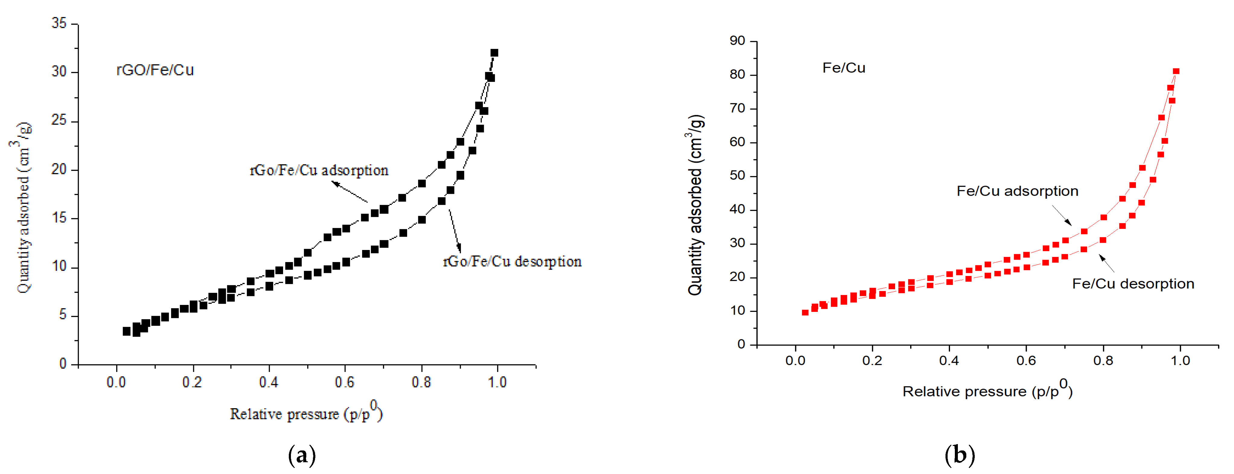
Figure 9.
The adsorption and desorption isotherms of the (a) Fe/Cu nanoparticles and (b) rGO/Fe/Cu nanocompounds.
Figure 9.
The adsorption and desorption isotherms of the (a) Fe/Cu nanoparticles and (b) rGO/Fe/Cu nanocompounds.
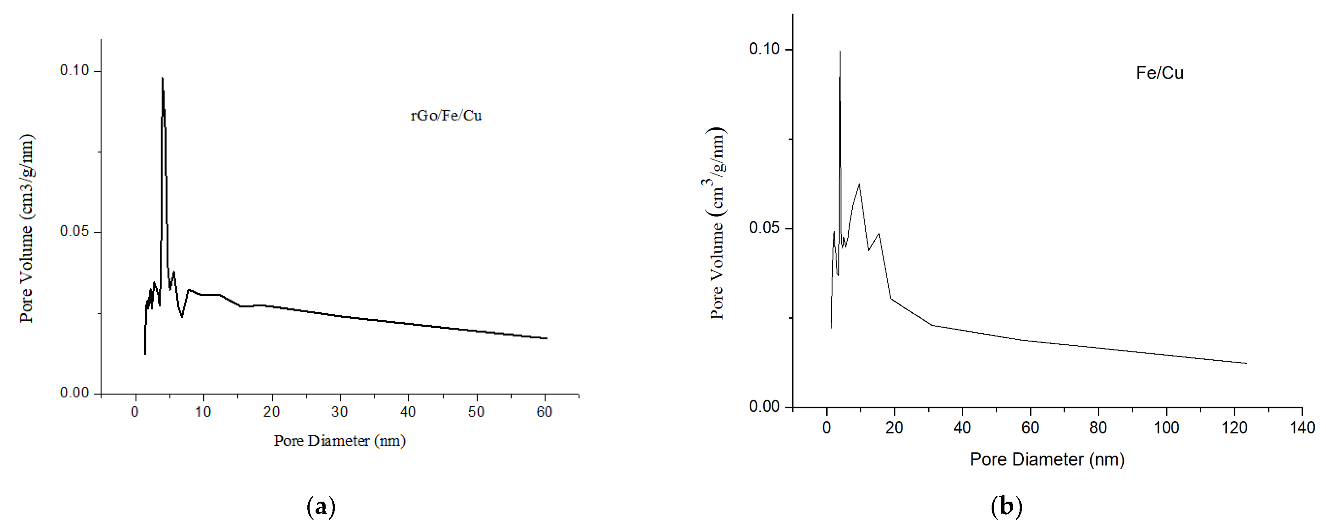
Figure 10.
BJH pore size distribution curves of the (a) Fe/Cu nanoparticles and (b) rGO/Fe/Cu nanocompounds.
Figure 10.
BJH pore size distribution curves of the (a) Fe/Cu nanoparticles and (b) rGO/Fe/Cu nanocompounds.
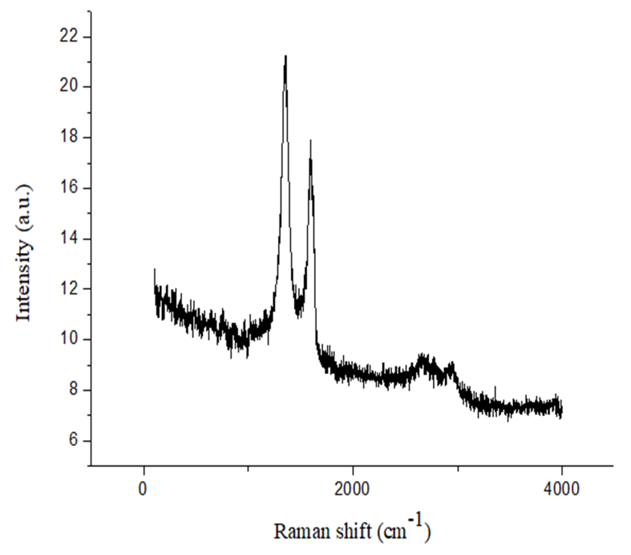
Figure 11.
Raman spectra of rGO/Fe/Cu nanocompounds.
Figure 11.
Raman spectra of rGO/Fe/Cu nanocompounds.
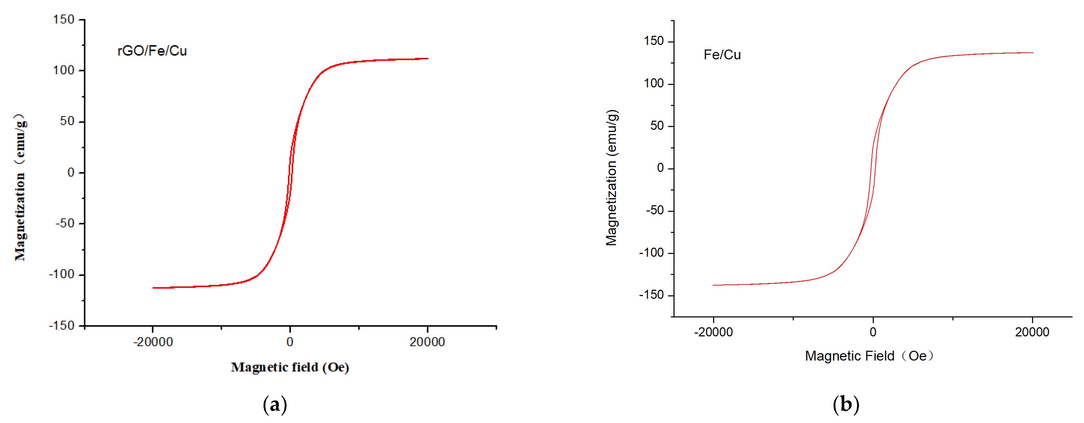
Figure 12.
Magnetization hysteresis loop of the (a) Fe/Cu nanoparticles and (b) rGO/Fe/Cu nanocompounds at room temperature.
Figure 12.
Magnetization hysteresis loop of the (a) Fe/Cu nanoparticles and (b) rGO/Fe/Cu nanocompounds at room temperature.
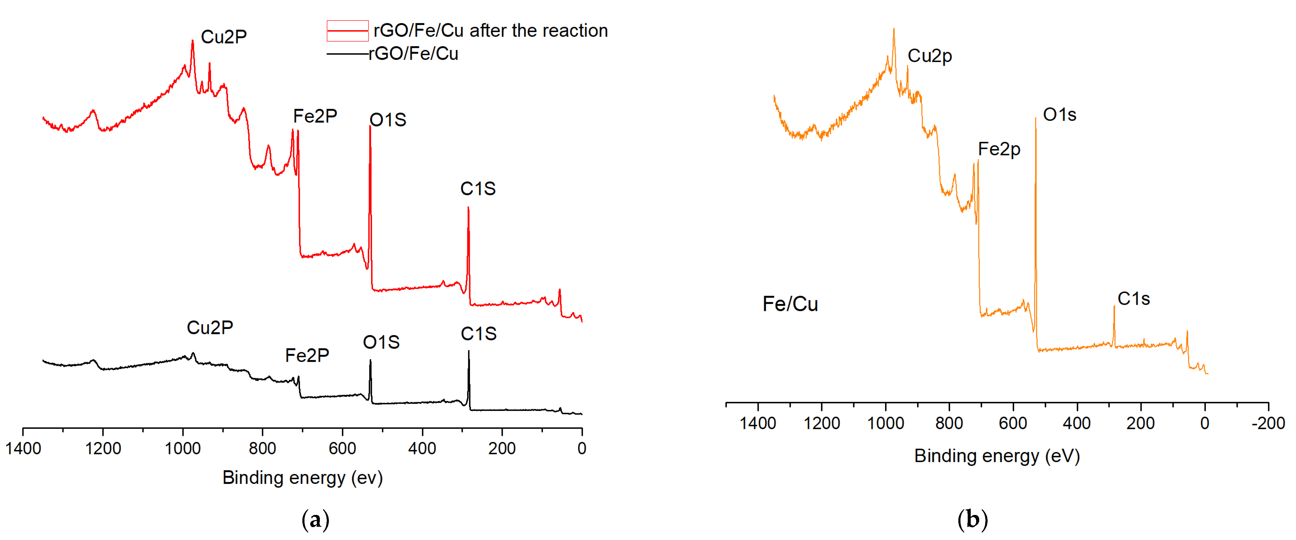
Figure 13.
Long-range XPS spectra of (a) Fe/Cu nanoparticles and (b) rGO/Fe/Cu nanocompounds.
Figure 13.
Long-range XPS spectra of (a) Fe/Cu nanoparticles and (b) rGO/Fe/Cu nanocompounds.
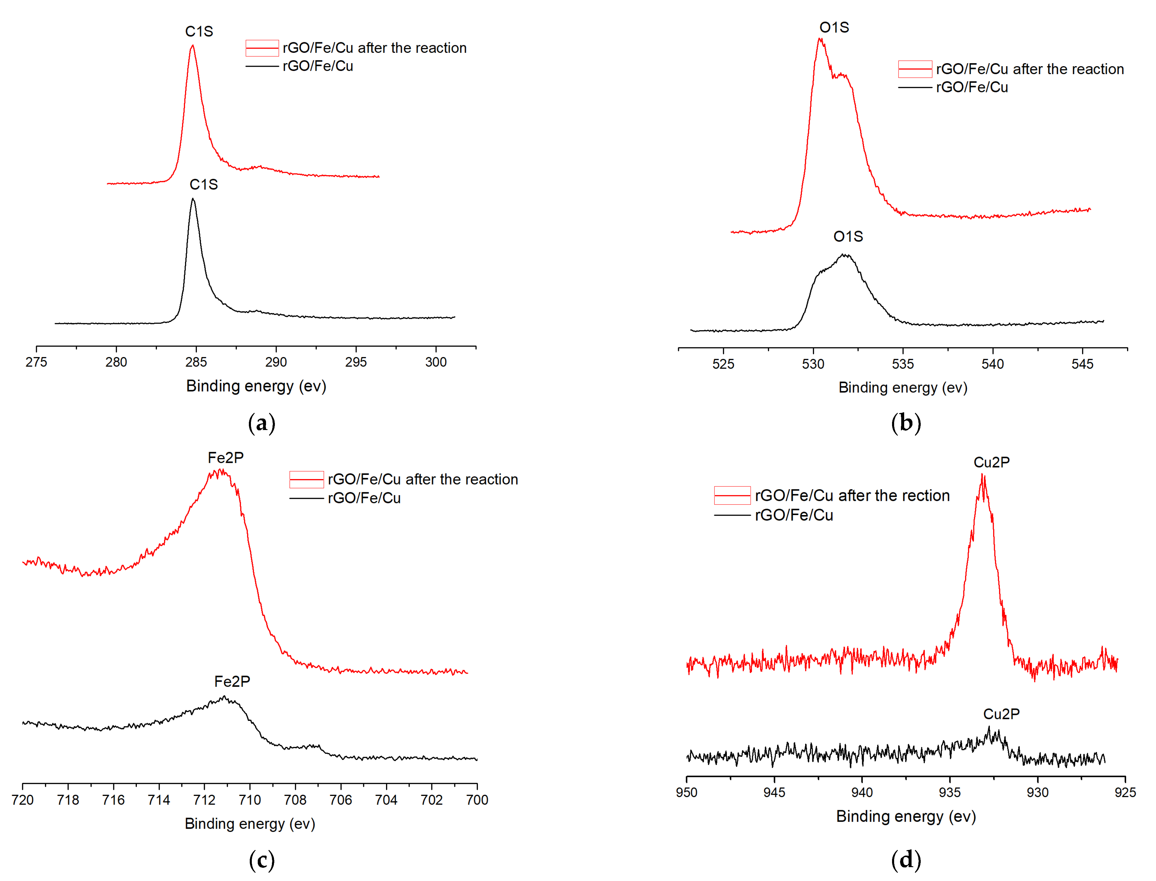
Figure 14.
Photoelectron spectra of (a) C(1S); (b) O(1S); (c) Fe(2P) and (d) Cu(2P) before and after removing carmine by rGO/Fe/Cu.
Figure 14.
Photoelectron spectra of (a) C(1S); (b) O(1S); (c) Fe(2P) and (d) Cu(2P) before and after removing carmine by rGO/Fe/Cu.
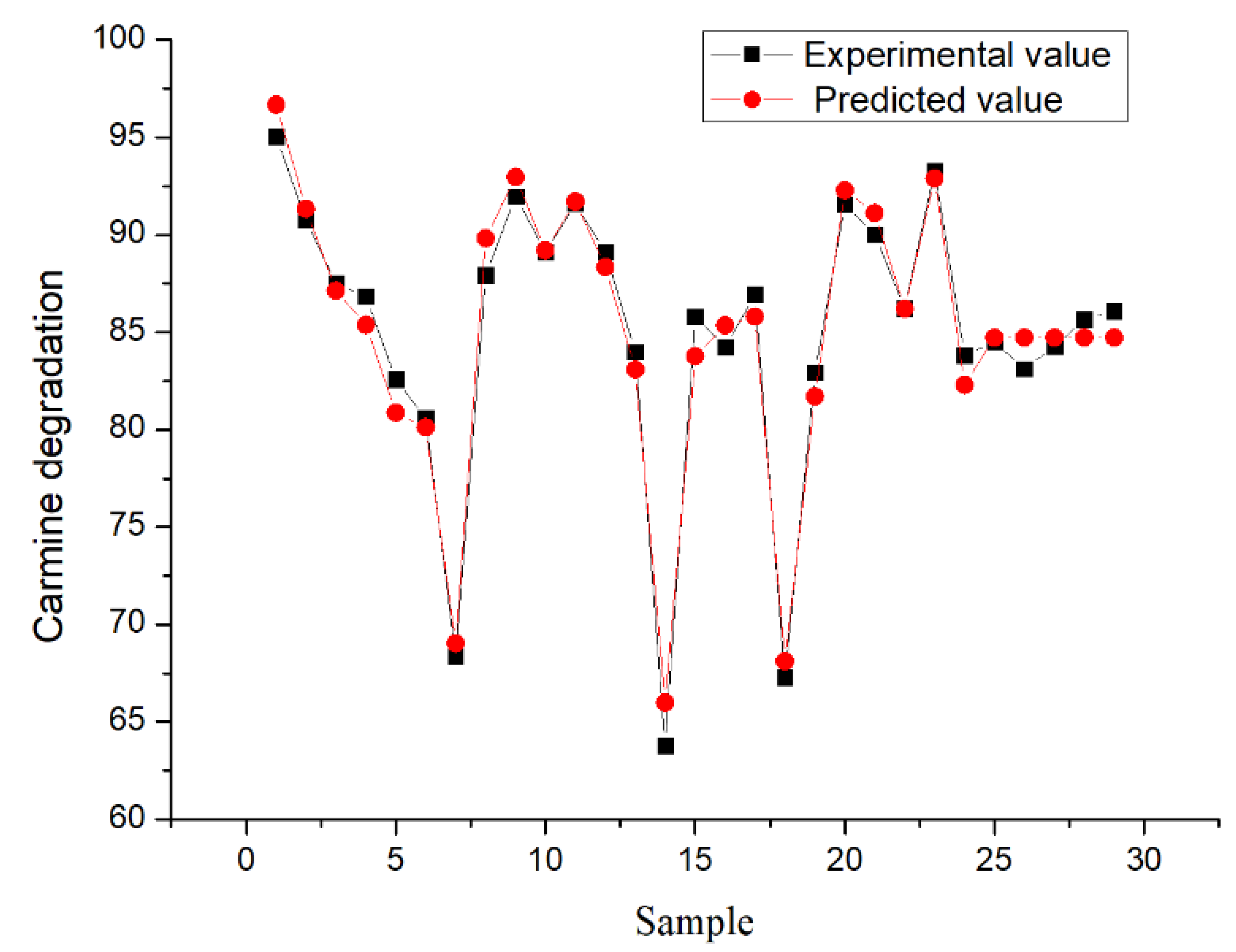
Figure 15.
Comparison of experimental and predicted values for RSM.
Figure 15.
Comparison of experimental and predicted values for RSM.
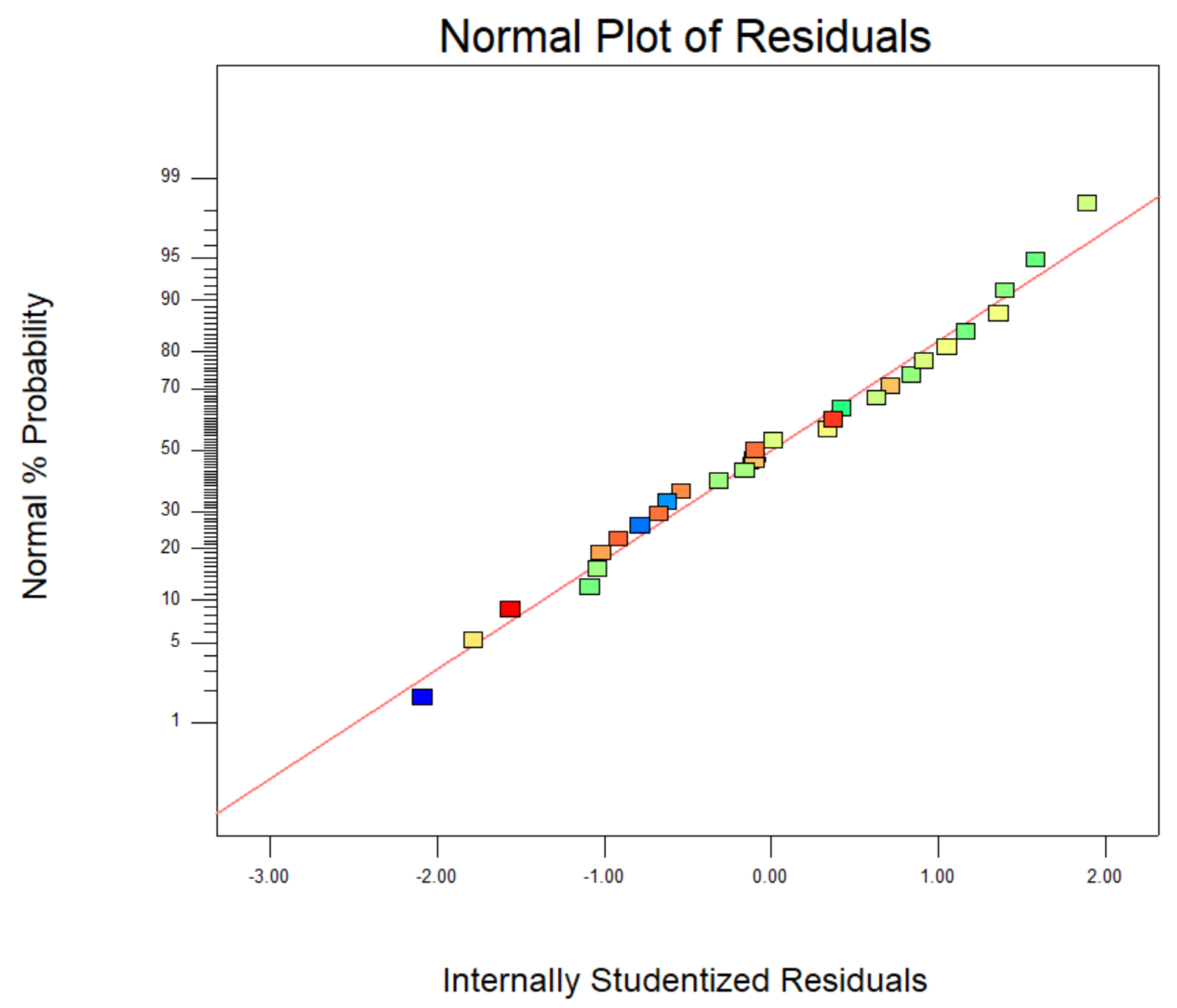
Figure 16.
Normal probabilities and internal learning residuals.
Figure 16.
Normal probabilities and internal learning residuals.
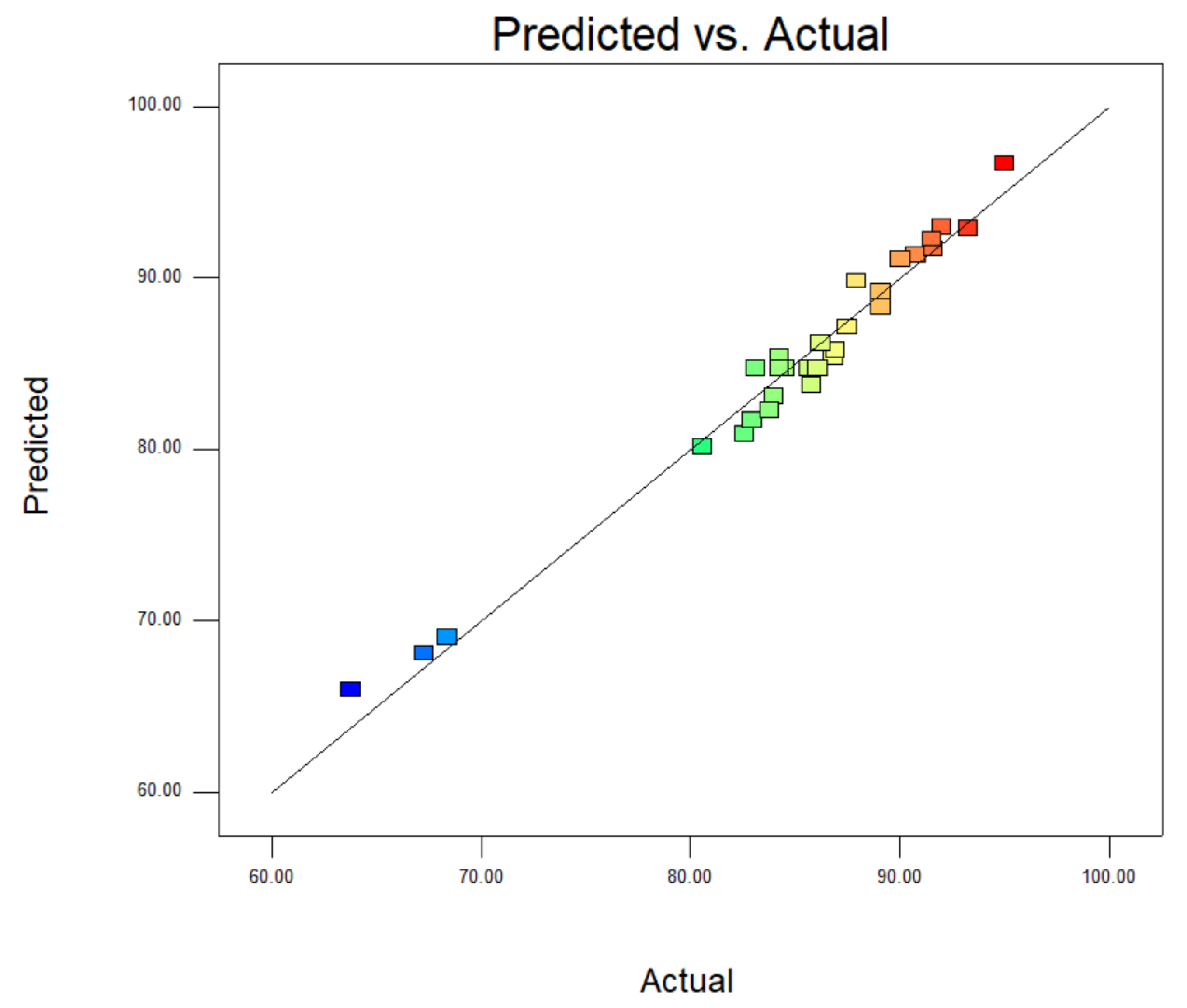
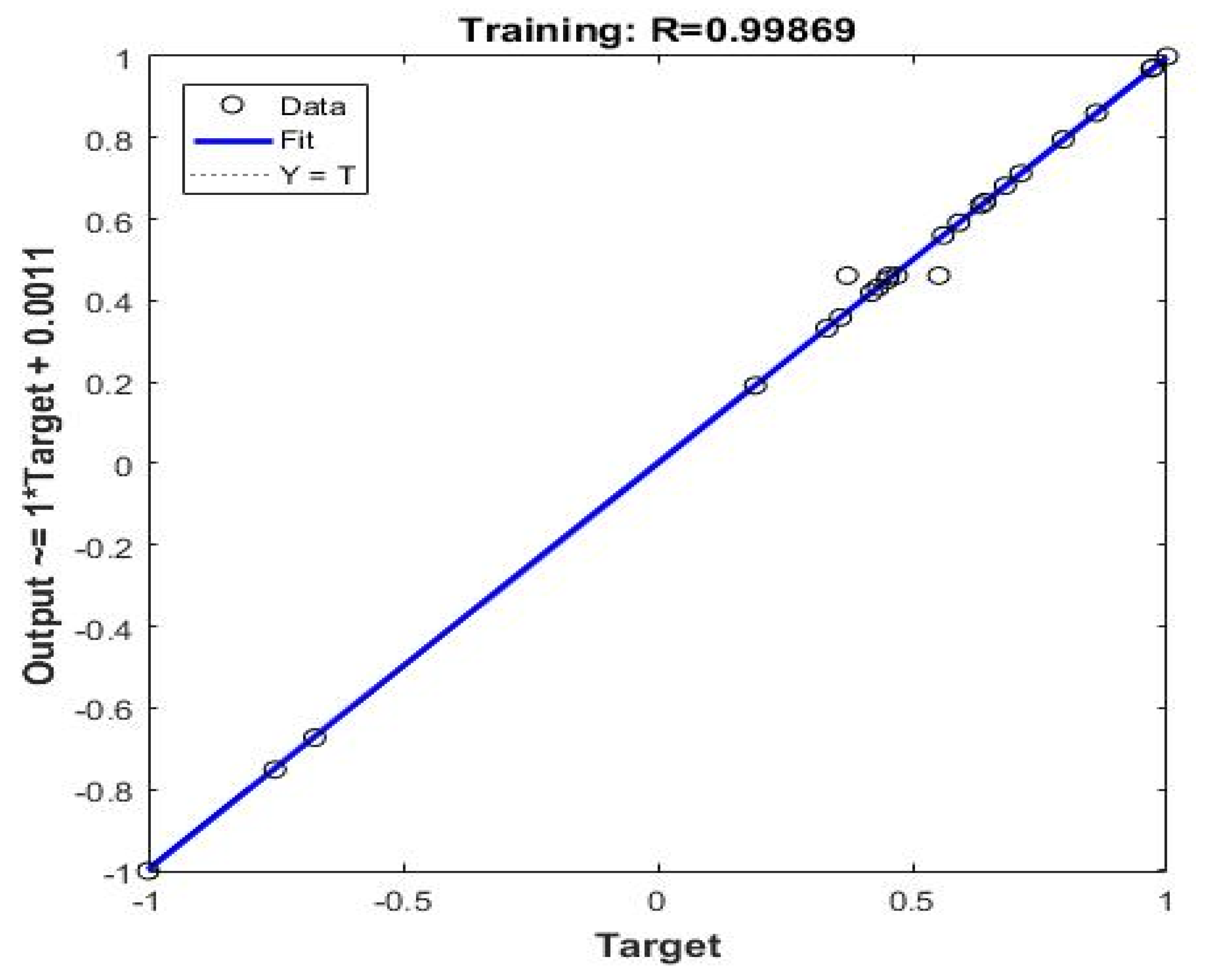
Figure 17.
Comparison of predicted and actual values.
Figure 17.
Comparison of predicted and actual values.
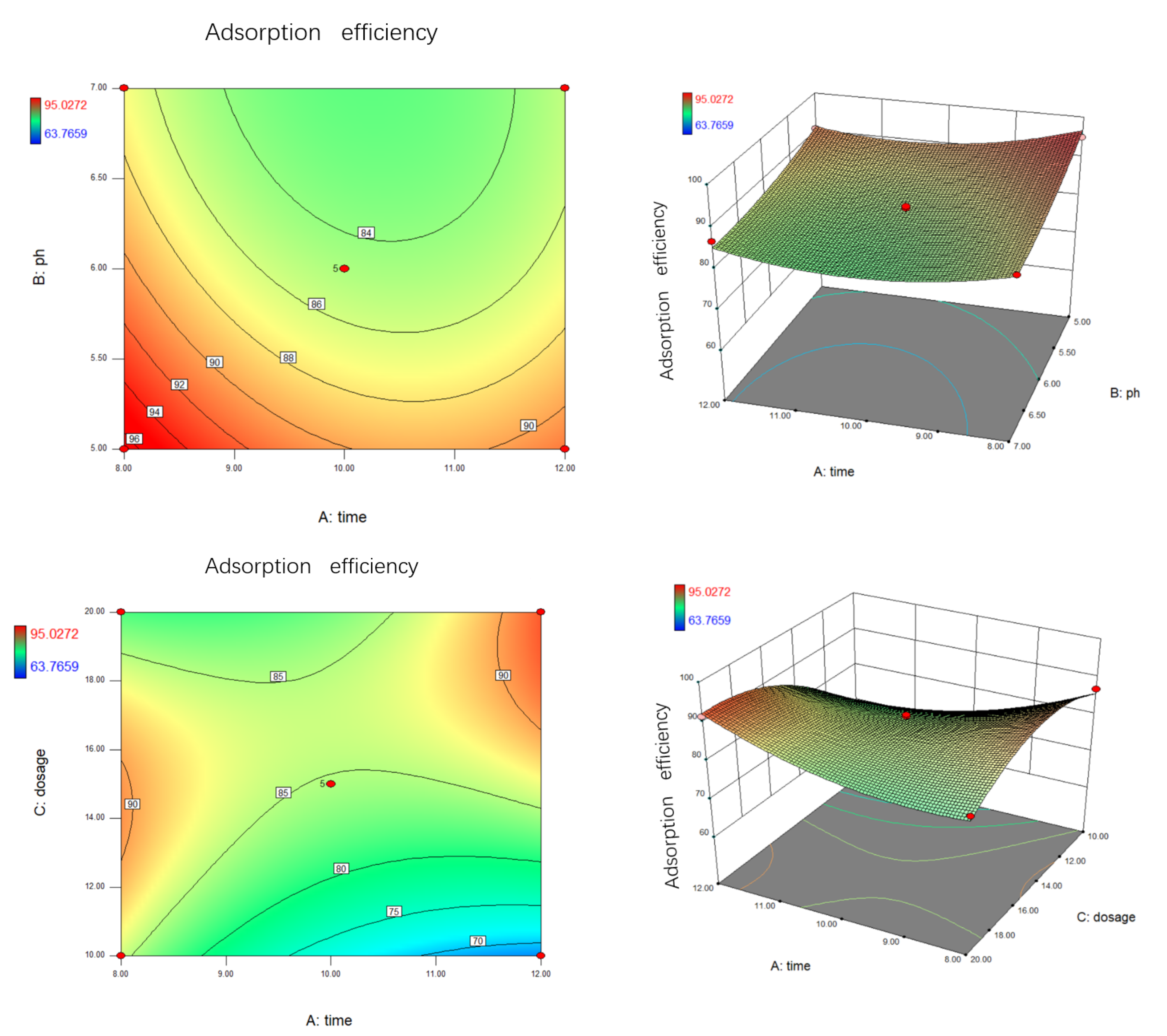
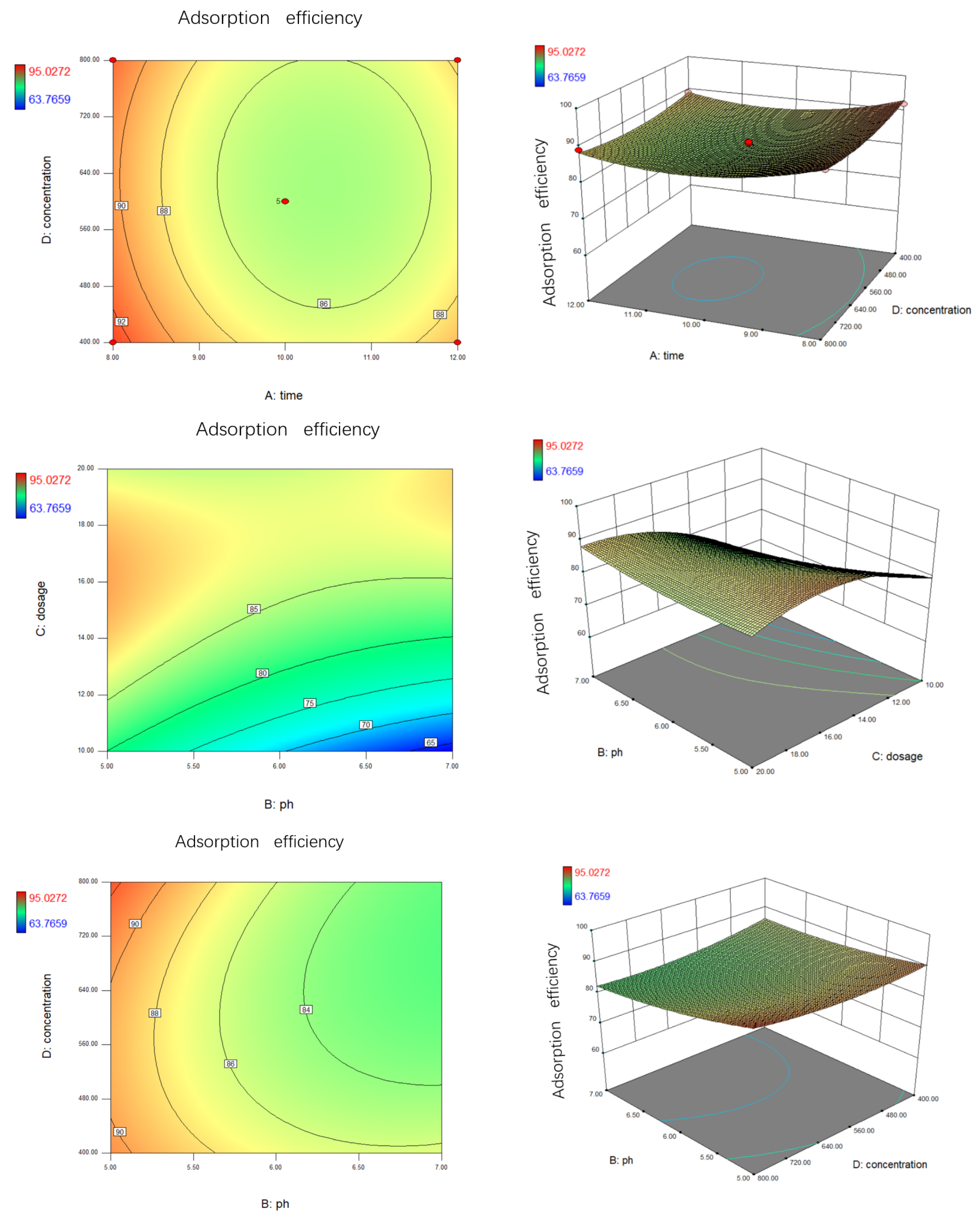
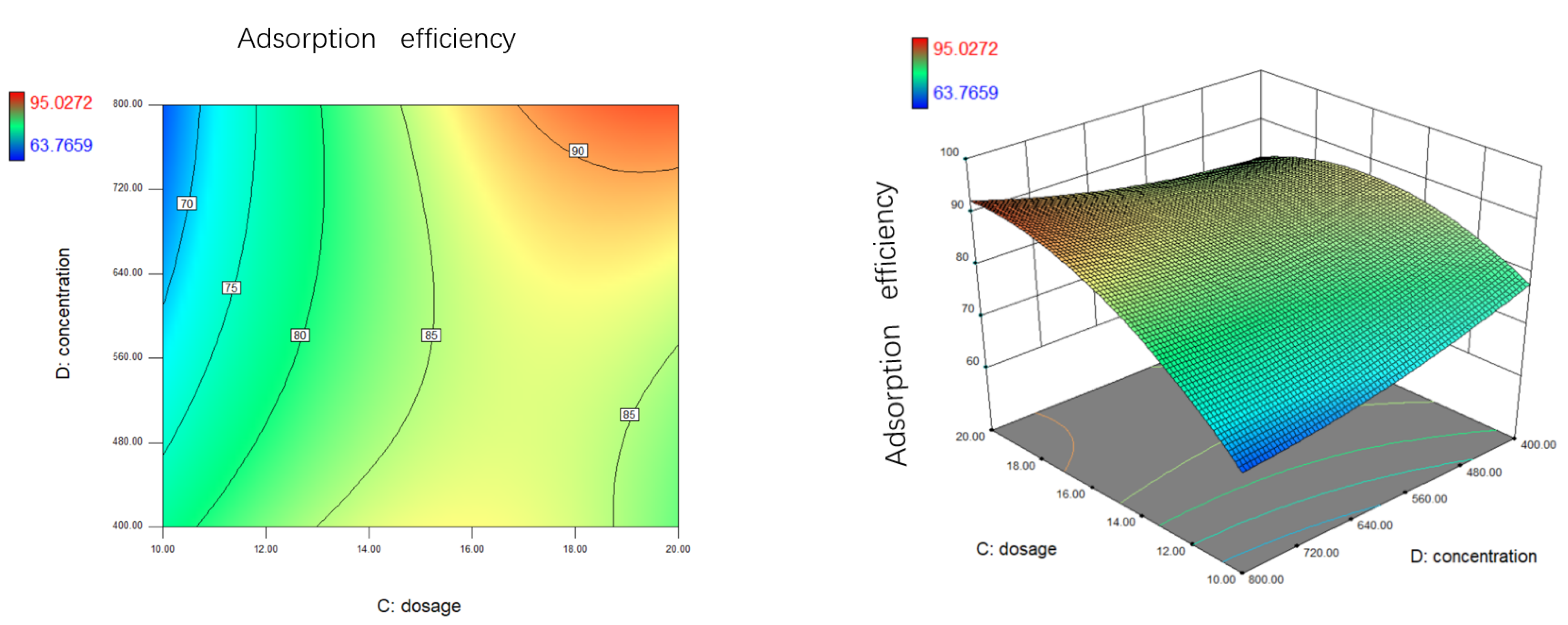
Figure 18.
The 3D response surface and 2D contour line map plots for carmine decontamination.
Figure 18.
The 3D response surface and 2D contour line map plots for carmine decontamination.
Figure 19.
The experimental and predicted data of normalized decontamination.
Figure 19.
The experimental and predicted data of normalized decontamination.
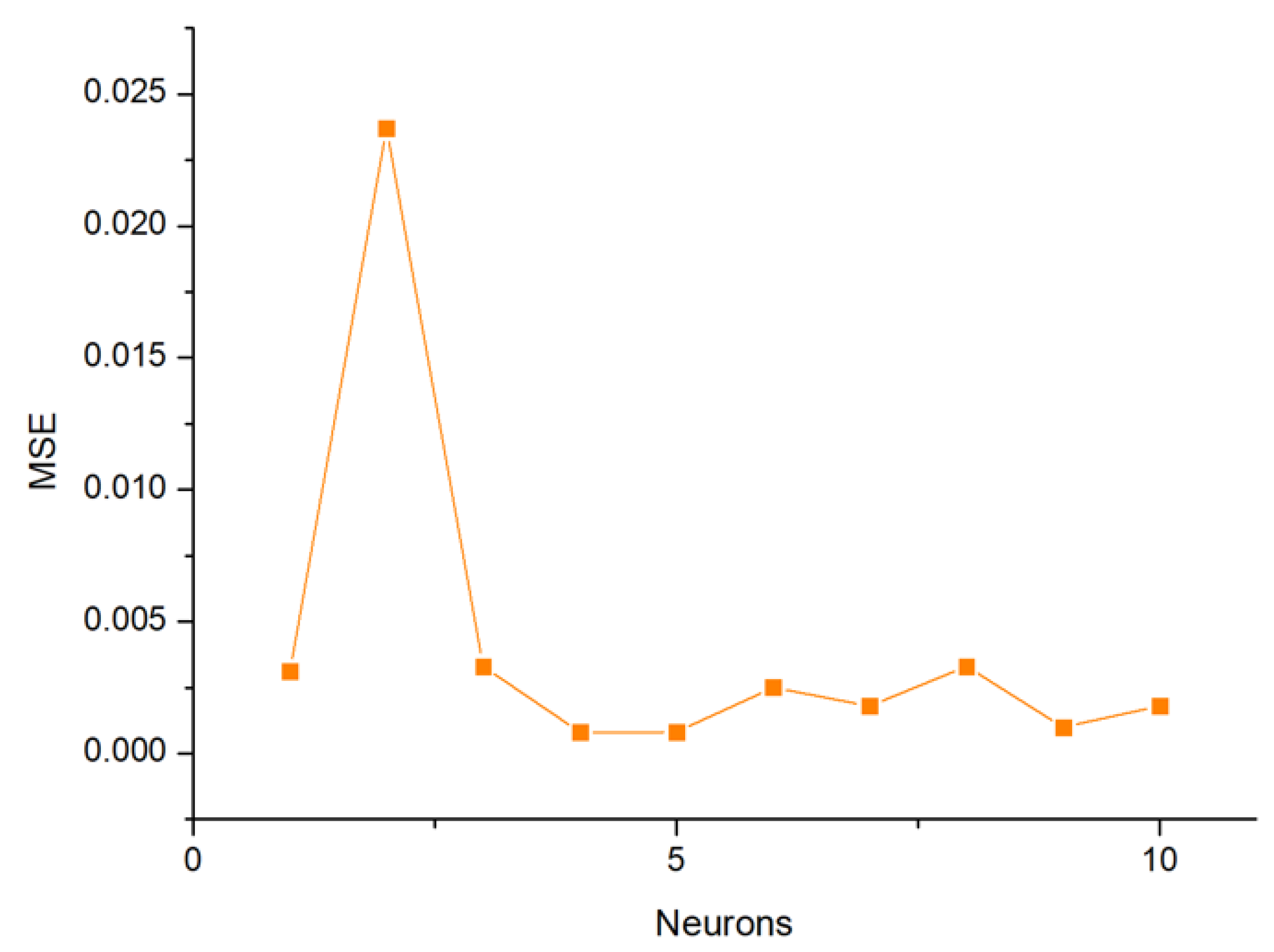
Figure 20.
Mean square error (MSE) of the neurons in the BP-ANN model.
Figure 20.
Mean square error (MSE) of the neurons in the BP-ANN model.
Figure 21.
A backpropagation artificial neural network schematic diagram.
Figure 21.
A backpropagation artificial neural network schematic diagram.
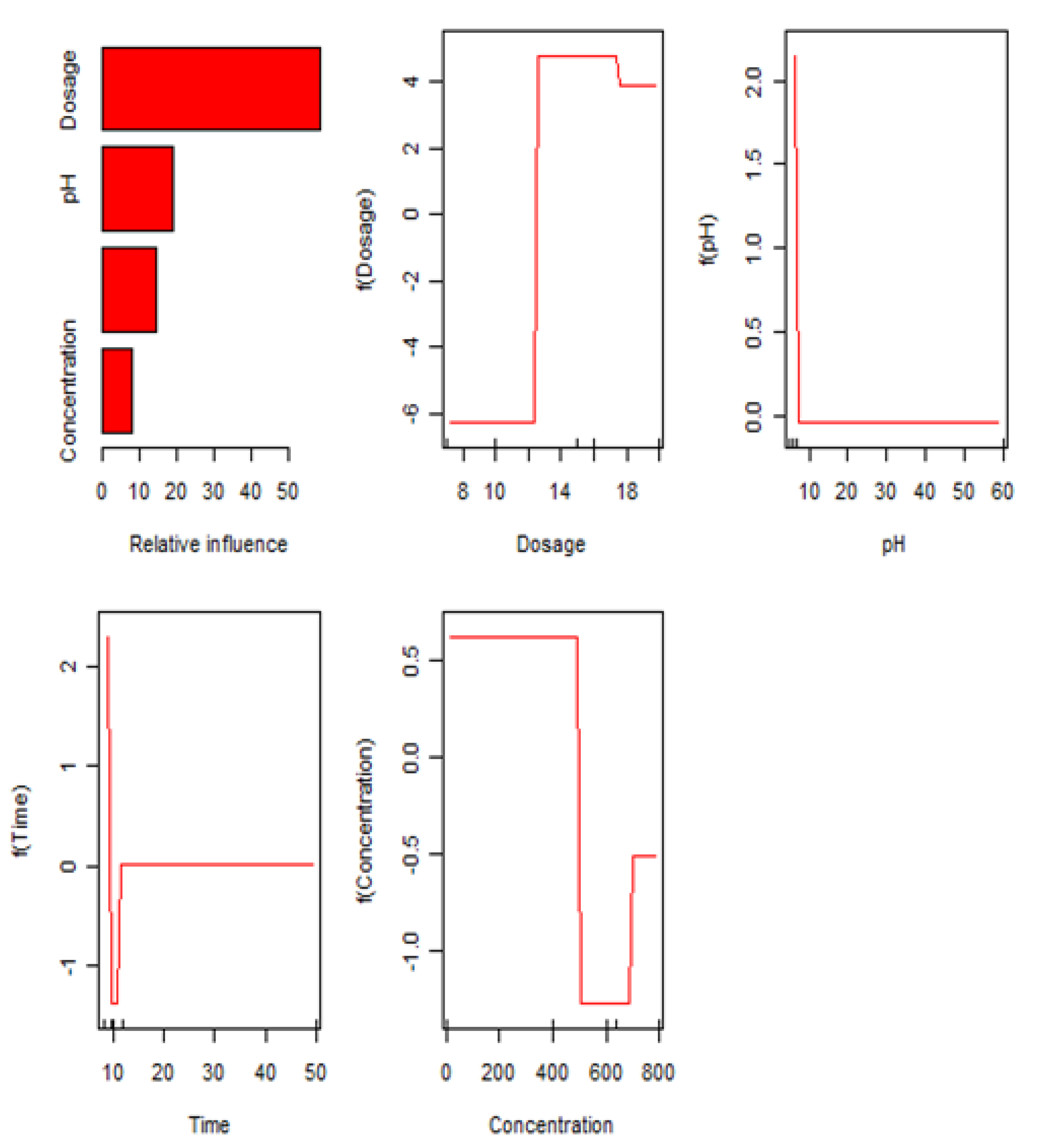
Figure 22.
The relative impact of the input variables obtained by R-studio.
Figure 22.
The relative impact of the input variables obtained by R-studio.
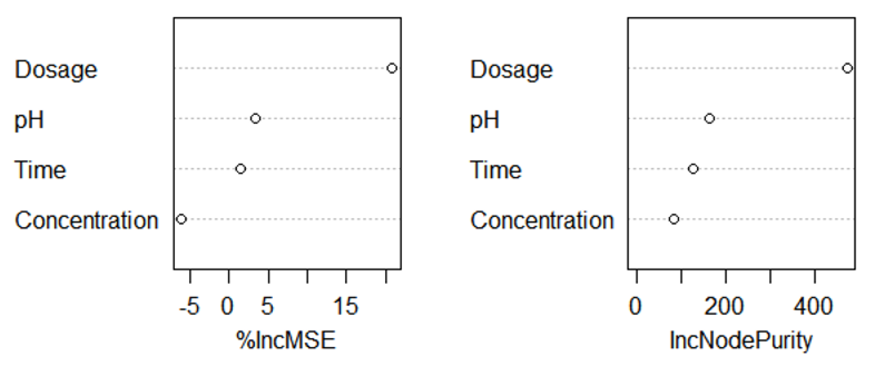
Figure 23.
The relative impact of the input variables obtained by R-gui.
Figure 23.
The relative impact of the input variables obtained by R-gui.
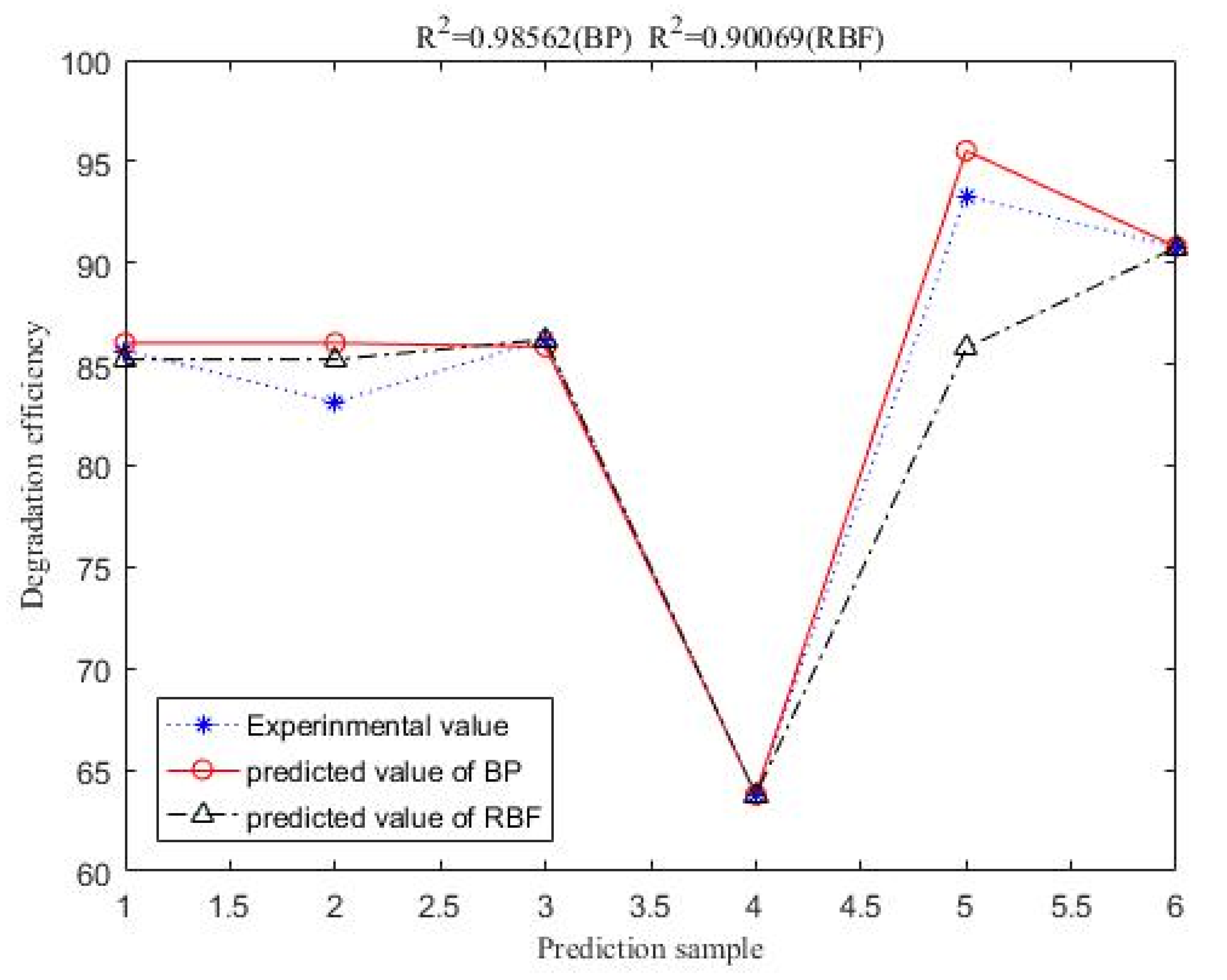
Figure 24.
Comparison of the predicted value of the radial basis function and the predicted value of BP with the experimental value.
Figure 24.
Comparison of the predicted value of the radial basis function and the predicted value of BP with the experimental value.
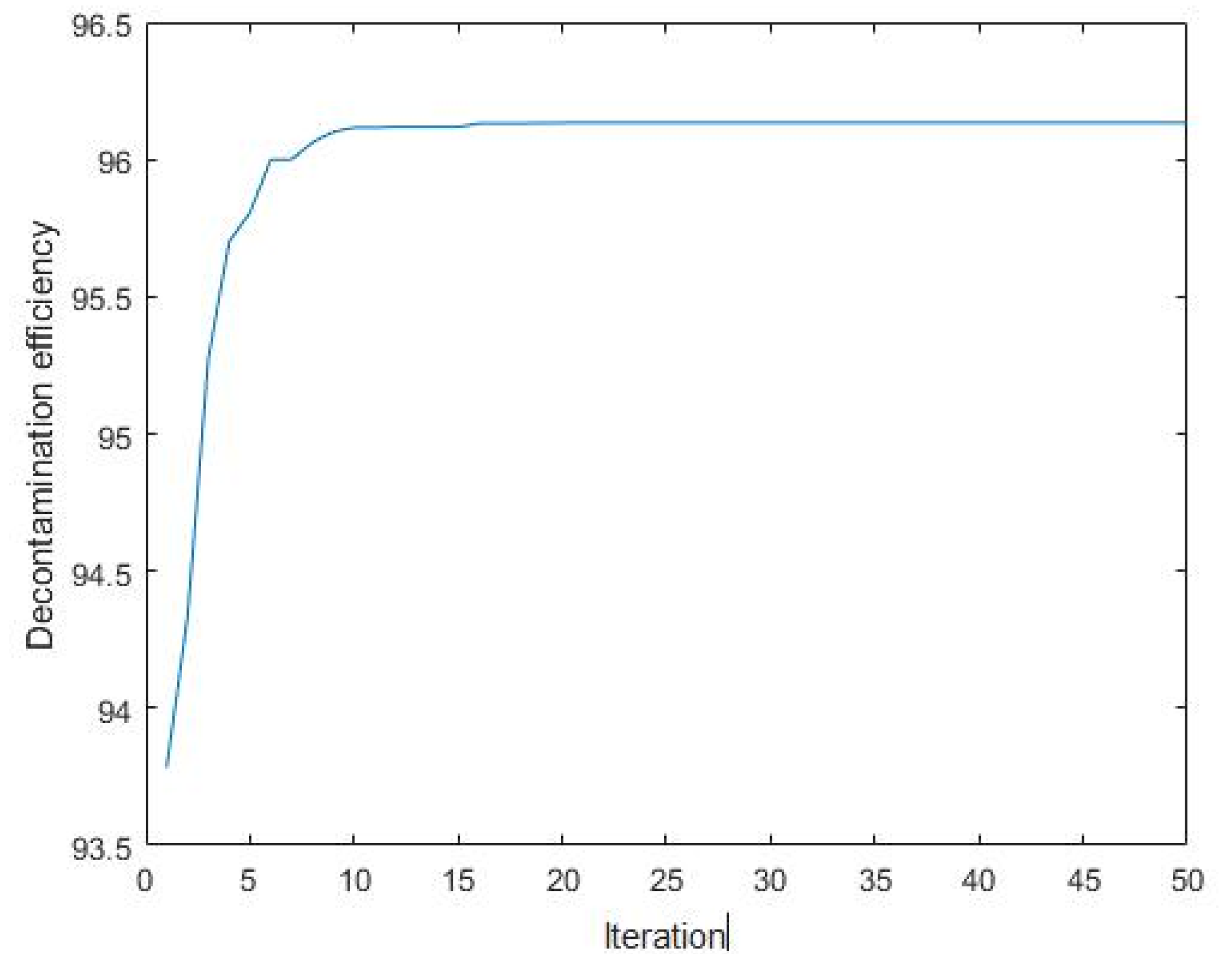
Figure 25.
Decontamination efficiency versus iteration.
Figure 25.
Decontamination efficiency versus iteration.
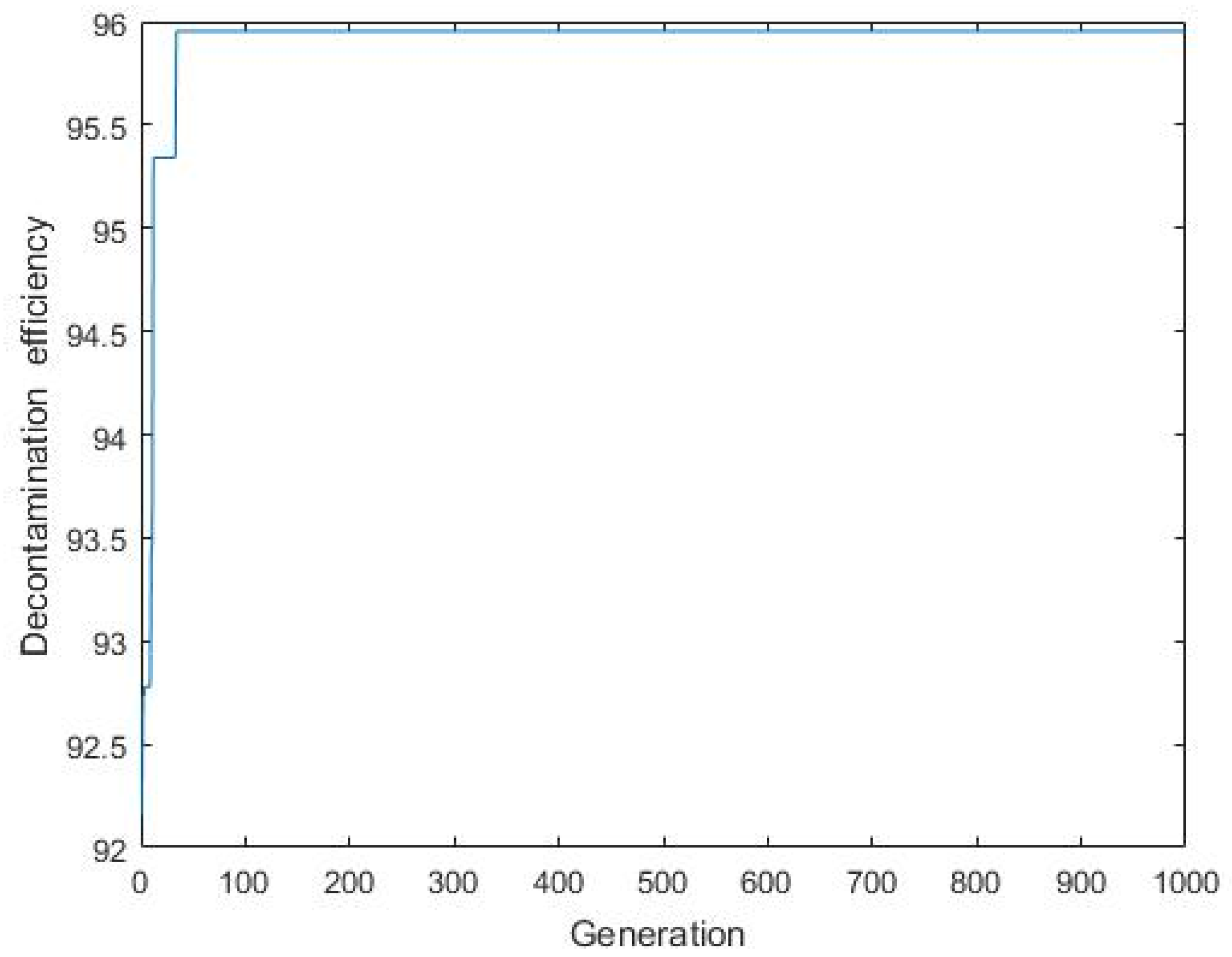
Figure 26.
Decontamination efficiency versus generation.
Figure 26.
Decontamination efficiency versus generation.
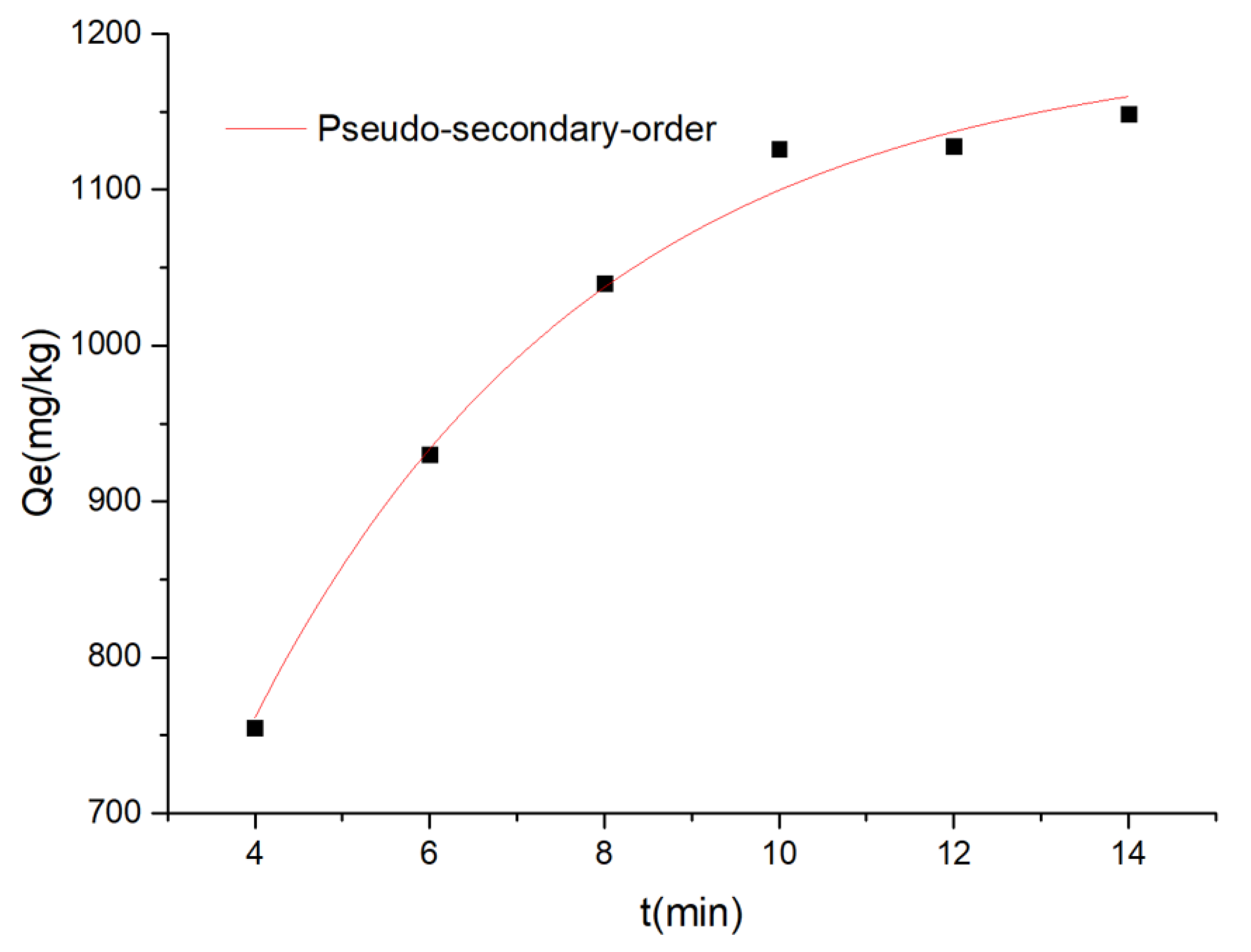
Figure 27.
Study on the pseudo-secondary kinetics of carmine removal by rGO/Fe/Cu.
Figure 27.
Study on the pseudo-secondary kinetics of carmine removal by rGO/Fe/Cu.
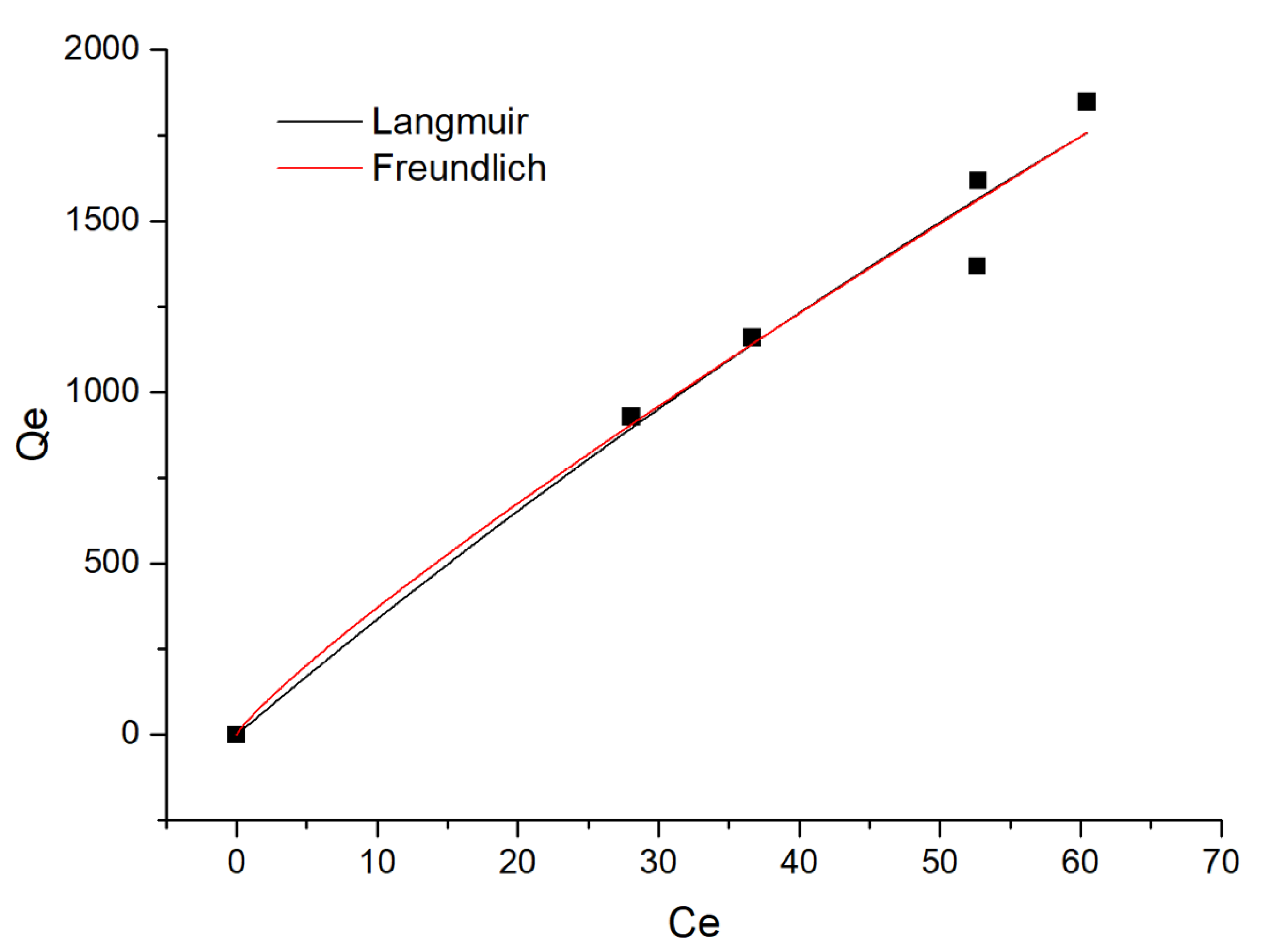
Figure 28.
Thermodynamic study on the removal of carmine by rGO/Fe/Cu.
Figure 28.
Thermodynamic study on the removal of carmine by rGO/Fe/Cu.
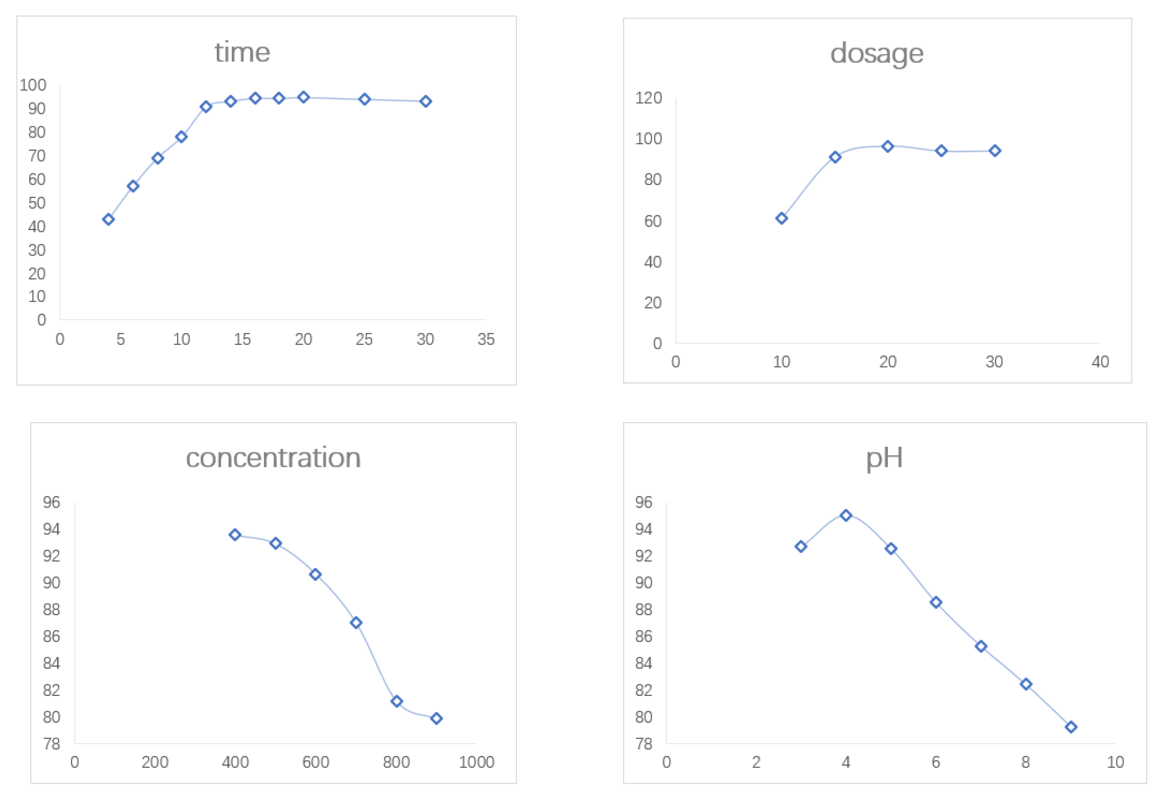
Figure 29.
The single-factor experimental curve of binary dyes.
Figure 29.
The single-factor experimental curve of binary dyes.
Table 1.
Chemical properties of carmine and Congo red.
Table 1.
Chemical properties of carmine and Congo red.
| Chemical Name | Carmine | Congo Red |
|---|
| Molecular formula | C20H11O10N2S3Na3 | C32H22N6Na2O6S2 |
| Molecular weight | 604 | 696.68 |
| Maximum wavelength λ | 509 nm | 497 nm |
| Solubility in water at 22 °C | ≥10 g/100 mg | ≥0.995 g/mL |
Table 2.
Independent variables and levels in the experimental design.
Table 2.
Independent variables and levels in the experimental design.
| Independent Variables | Unit | Code | Coded Variable Levels |
|---|
| −1 | 0 | 1 |
|---|
| Contact time | min | A | 8 | 10 | 12 |
| pH | - | B | 5 | 6 | 7 |
| Dosage | mg | C | 10 | 15 | 20 |
| Concentration | mg/L | D | 400 | 600 | 800 |
Table 3.
Comparison of the decontamination efficiency predicted by the BBD model with the experimental values.
Table 3.
Comparison of the decontamination efficiency predicted by the BBD model with the experimental values.
| Run | A (min) | B | C (mg) | D (mg/L) | Actual Value (%) | Predicted Value (%) | Absolute Error (%) |
|---|
| 1 | 10 | 5 | 10 | 600 | 90.76 | 91.34 | 0.58 |
| 2 | 10 | 7 | 15 | 800 | 87.50 | 87.14 | 0.36 |
| 3 | 10 | 7 | 20 | 600 | 86.84 | 85.38 | 1.46 |
| 4 | 10 | 5 | 20 | 600 | 82.57 | 80.87 | 1.70 |
| 5 | 10 | 6 | 20 | 400 | 80.58 | 80.13 | 0.45 |
| 6 | 10 | 6 | 15 | 600 | 68.38 | 69.04 | 0.66 |
| 7 | 12 | 6 | 10 | 600 | 87.93 | 89.83 | 1.90 |
| 8 | 12 | 6 | 20 | 600 | 91.99 | 92.96 | 0.97 |
| 9 | 10 | 6 | 15 | 600 | 89.11 | 89.21 | 0.10 |
| 10 | 12 | 6 | 15 | 800 | 91.61 | 91.71 | 0.10 |
| 11 | 10 | 6 | 10 | 400 | 89.11 | 88.34 | 0.77 |
| 12 | 10 | 7 | 15 | 400 | 83.98 | 83.08 | 0.90 |
| 13 | 10 | 6 | 10 | 800 | 63.77 | 65.99 | 2.22 |
| 14 | 10 | 6 | 20 | 800 | 85.79 | 83.77 | 2.02 |
| 15 | 10 | 6 | 15 | 600 | 84.24 | 85.35 | 1.11 |
| 16 | 8 | 6 | 15 | 400 | 86.94 | 85.81 | 1.13 |
| 17 | 8 | 6 | 20 | 600 | 67.28 | 68.11 | 0.83 |
| 18 | 10 | 6 | 15 | 600 | 82.94 | 81.70 | 1.24 |
| 19 | 8 | 7 | 15 | 600 | 91.56 | 92.28 | 0.72 |
| 20 | 10 | 7 | 10 | 600 | 90.03 | 91.12 | 1.09 |
| 21 | 8 | 6 | 10 | 600 | 86.22 | 86.21 | 0.01 |
| 22 | 12 | 7 | 15 | 600 | 93.30 | 92.90 | 0.40 |
| 23 | 10 | 5 | 15 | 400 | 83.80 | 82.30 | 1.50 |
| 24 | 8 | 6 | 15 | 800 | 84.50 | 84.73 | 0.23 |
| 25 | 10 | 6 | 15 | 600 | 83.13 | 84.73 | 1.60 |
| 26 | 10 | 5 | 15 | 800 | 84.27 | 84.73 | 0.46 |
| 27 | 12 | 5 | 15 | 600 | 85.67 | 84.73 | 0.94 |
| 28 | 8 | 5 | 15 | 600 | 86.08 | 84.73 | 1.35 |
| 29 | 12 | 6 | 15 | 400 | 90.76 | 91.34 | 0.58 |
| Mean absolute error (%) | 0.87 |
Table 4.
Analysis of variance (ANOVA) for the response surface quadratic model.
Table 4.
Analysis of variance (ANOVA) for the response surface quadratic model.
| Source | Sum of Squares | Degree of Freedom | Mean Square | F-Value | p-Value | Significant or Not Significant |
|---|
| Model | 1462.943 | 14 | 104.4959 | 38.19779 | <0.0001 | Significant |
| A (Time) | 38.00306 | 1 | 38.00306 | 13.89177 | 0.0023 | |
| B (pH) | 180.3591 | 1 | 180.3591 | 65.9291 | <0.0001 | |
| C (Dosage) | 301.4176 | 1 | 301.4176 | 110.1812 | <0.0001 | |
| D (Concentration) | 3.381933 | 1 | 3.381933 | 1.236243 | 0.2849 | |
| AB | 3.228349 | 1 | 3.228349 | 1.180102 | 0.2957 | |
| AC | 199.9882 | 1 | 199.9882 | 73.10439 | <0.0001 | |
| AD | 0.036267 | 1 | 0.036267 | 0.013257 | 0.9100 | |
| BC | 87.15988 | 1 | 87.15988 | 31.86073 | <0.0001 | |
| BD | 8.11368 | 1 | 8.11368 | 2.965903 | 0.1070 | |
| CD | 115.9419 | 1 | 115.9419 | 42.38182 | <0.0001 | |
| A2 | 99.51958 | 1 | 99.51958 | 36.37873 | <0.0001 | |
| B2 | 14.43986 | 1 | 14.43986 | 5.278395 | 0.0375 | |
| C2 | 288.5931 | 1 | 288.5931 | 105.4933 | <0.0001 | |
| D2 | 23.70787 | 1 | 23.70787 | 8.666257 | 0.0107 | |
| Residual | 38.29914 | 14 | 2.735653 | | | |
| Lack of Fit | 32.74903 | 10 | 3.274903 | 2.360244 | 0.2116 | Not Significant |
| Pure Error | 5.550108 | 4 | 1.387527 | | | |
| Cor Total | 1501.242 | 28 | | | | |
Table 5.
The experimental design matrix of the backpropagation (BP) artificial neural network (ANN) model.
Table 5.
The experimental design matrix of the backpropagation (BP) artificial neural network (ANN) model.
| Runs | X1 (min) | X2 | X3 (mg) | X4 (mg/L) | Experimental Value (%) | Predicted Value (%) |
|---|
| 1 | 10 | 5 | 10 | 600 | 83.9843 | 81.9819 |
| 2 | 10 | 7 | 15 | 800 | 83.7990 | 85.0323 |
| 3 | 10 | 7 | 20 | 600 | 84.2445 | 83.4627 |
| 4 | 10 | 5 | 20 | 600 | 85.7910 | 88.5915 |
| 5 | 10 | 6 | 20 | 400 | 80.5823 | 86.7515 |
| 6 | 10 | 6 | 15 | 600 | 84.2665 | 85.1908 |
| 7 | 12 | 6 | 10 | 600 | 67.2769 | 83.0775 |
| 8 | 12 | 6 | 20 | 600 | 91.5635 | 84.6104 |
| 9 | 10 | 6 | 15 | 600 | 83.1270 | 85.3418 |
| 10 | 12 | 6 | 15 | 800 | 89.1085 | 85.7064 |
| 11 | 10 | 6 | 10 | 400 | 82.5666 | 80.6683 |
| 12 | 10 | 7 | 15 | 400 | 86.2249 | 85.1616 |
| 13 | 10 | 6 | 10 | 800 | 68.3817 | 82.6676 |
| 14 | 10 | 6 | 20 | 800 | 87.9326 | 85.2220 |
| 15 | 10 | 6 | 15 | 600 | 85.6656 | 85.0334 |
| 16 | 8 | 6 | 15 | 400 | 91.9886 | 87.1420 |
| 17 | 8 | 6 | 20 | 600 | 82.9441 | 88.2917 |
| 18 | 10 | 6 | 15 | 600 | 84.4953 | 84.4836 |
| 19 | 8 | 7 | 15 | 600 | 87.5047 | 85.6040 |
| 20 | 10 | 7 | 10 | 600 | 63.7659 | 80.8439 |
| 21 | 8 | 6 | 10 | 600 | 86.9410 | 80.3149 |
| 22 | 12 | 7 | 15 | 600 | 86.8359 | 84.3499 |
| 23 | 10 | 5 | 15 | 400 | 90.0294 | 88.1946 |
| 24 | 8 | 6 | 15 | 800 | 91.6078 | 86.8738 |
| 25 | 10 | 6 | 15 | 600 | 86.0846 | 85.5328 |
| * 26 | 10 | 5 | 15 | 800 | 93.3004 | 87.2787 |
| * 27 | 12 | 5 | 15 | 600 | 90.7649 | 87.8442 |
| * 28 | 8 | 5 | 15 | 600 | 95.0272 | 88.0859 |
| * 29 | 12 | 6 | 15 | 400 | 89.1085 | 86.5487 |
Table 6.
Weights and biases of the BP-ANN in the input hidden layers (wi and bi) and the hidden output layers (wj and bj).
Table 6.
Weights and biases of the BP-ANN in the input hidden layers (wi and bi) and the hidden output layers (wj and bj).
| Number of Neurons | wi | Input Bias | Layer Weights | Layer Bias |
|---|
| Input Weights |
|---|
| Contact Time | Initial pH | Dosage | Concentration |
|---|
| 1 | 1.4272 | −1.4802 | 0.9073 | 2.4895 | 2.4895 | 0.7555 | −0.1334 |
| 2 | −1.7844 | −1.6223 | 0.1750 | −1.9363 | −1.9363 | 0.7555 |
| 3 | 1.4870 | 1.4928 | 0.5855 | −1.3831 | −1.3831 | 0.7555 |
| 4 | −1.1910 | 0.5800 | 1.5085 | 0.8298 | 0.8298 | 0.7555 |
| 5 | 0.6114 | −0.9833 | −1.6289 | −0.2766 | −0.2766 | 0.7555 |
| 6 | 0.4390 | −0.4901 | −0.9972 | 0.2766 | 0.2766 | 0.7555 |
| 7 | 0.6983 | −1.5074 | −1.8098 | 0.8298 | 0.8298 | 0.7555 |
| 8 | −0.5684 | −0.9470 | −1.2455 | −1.3831 | −1.3831 | 0.7555 |
| 9 | 0.7825 | −1.5754 | 1.4324 | −1.9363 | −1.9363 | 0.7555 |
| 10 | 1.6152 | −0.8738 | 1.1511 | −2.4895 | −2.4895 | 0.7555 |
Table 7.
The relative influence of the input variables.
Table 7.
The relative influence of the input variables.
| Input Variables | Relative Significance (%) | Order |
|---|
| Contact Time | 14.44% | 3 |
| Initial pH | 18.96% | 2 |
| Dosage | 58.35% | 1 |
| Concentration | 8.23% | 4 |
Table 8.
Comparison of the predicted percentage of decontamination of carmine by the BBD, ANN-PSO and ANN-GA models with the experimental results.
Table 8.
Comparison of the predicted percentage of decontamination of carmine by the BBD, ANN-PSO and ANN-GA models with the experimental results.
| Models | Independent Parameters | Prediction (%) | Experiment (%) | Absolute Error (%) |
|---|
| A | B | C | D |
|---|
| BBD | 8.43 | 5.09 | 14.30 | 437.4 | 95.80 | 93.28 | 2.52 |
| ANN-PSO | 12.00 | 5.31 | 16.62 | 764.3 | 96.13 | 95.79 | 0.34 |
| ANN-GA | 8.01 | 5.85 | 14.49 | 581.3 | 95.84 | 92.17 | 3.67 |
Table 9.
The R2 values of the kinetics for carmine adsorption on rGO/Fe/Cu nanohybrids.
Table 9.
The R2 values of the kinetics for carmine adsorption on rGO/Fe/Cu nanohybrids.
| Kinetic Models | Values of R2 |
|---|
| Pseudo-first-order | 0.9897 |
| Pseudo-second-order | 0.9931 |
| Intraparticle diffusion | 0.9044 |
| Elovich | 0.9496 |
Table 10.
Rules for judging the type of adsorption isotherm by RL value.
Table 10.
Rules for judging the type of adsorption isotherm by RL value.
| Values of RL | Type of Adsorption Nature |
|---|
| RL > 1 | Unfavorable |
| RL = 1 | Linear |
| 0 < RL < 1 | Favorable |
| RL = 0 | Irreversible |
Table 11.
The R2 values of the thermodynamics for carmine adsorption onto rGO/Fe/Cu nanohybrids.
Table 11.
The R2 values of the thermodynamics for carmine adsorption onto rGO/Fe/Cu nanohybrids.
| Thermodynamics Models | Values of R2 |
|---|
| Langmuir | 0.8704 |
| Freundlich | 0.9709 |
| Temkin | 0.8837 |


 and
and 


