A Hybrid Modeling of the Physics-Driven Evolution of Material Addition and Track Generation in Laser Powder Directed Energy Deposition


Abstract
:1. Introduction
2. Analysis of the LP-DED Process
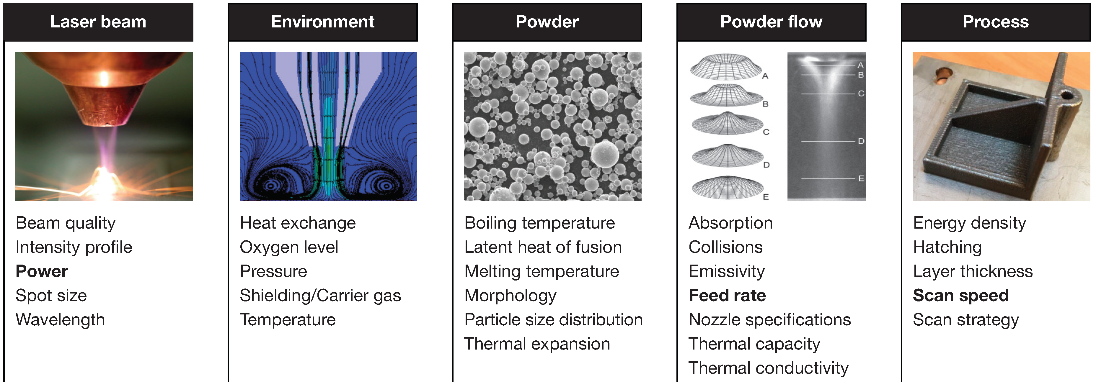
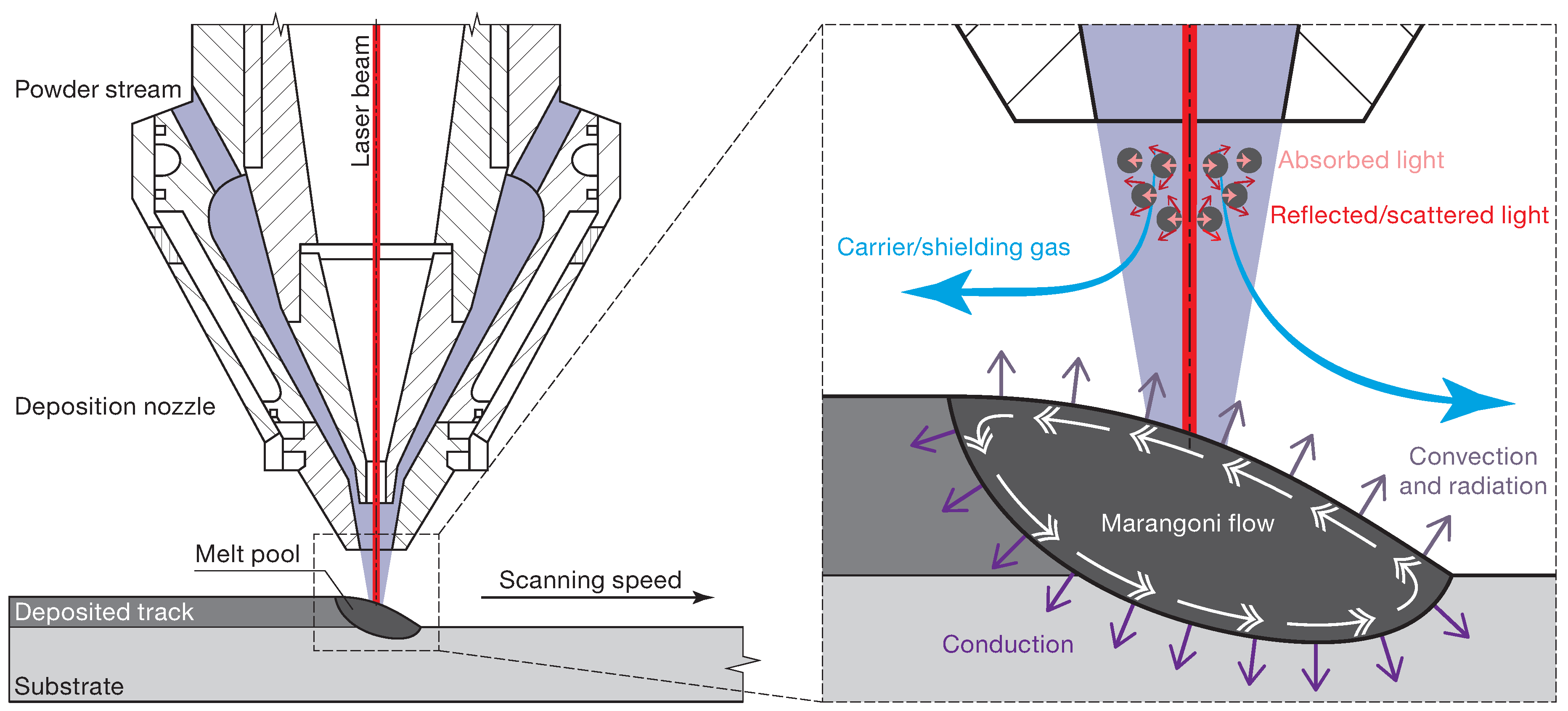
2.1. Physics of the LP-DED Process
2.1.1. The Powder Stream Process
2.1.2. The Melt Pool Generation
2.1.3. The Solidification of the Track
2.2. Modeling of the LP-DED Process
3. The Hybrid Analytic-Numerical Model of the LP-DED Process
3.1. Heat Transfer Modeling
3.1.1. Heat Conduction
3.1.2. Convection
3.1.3. Radiation
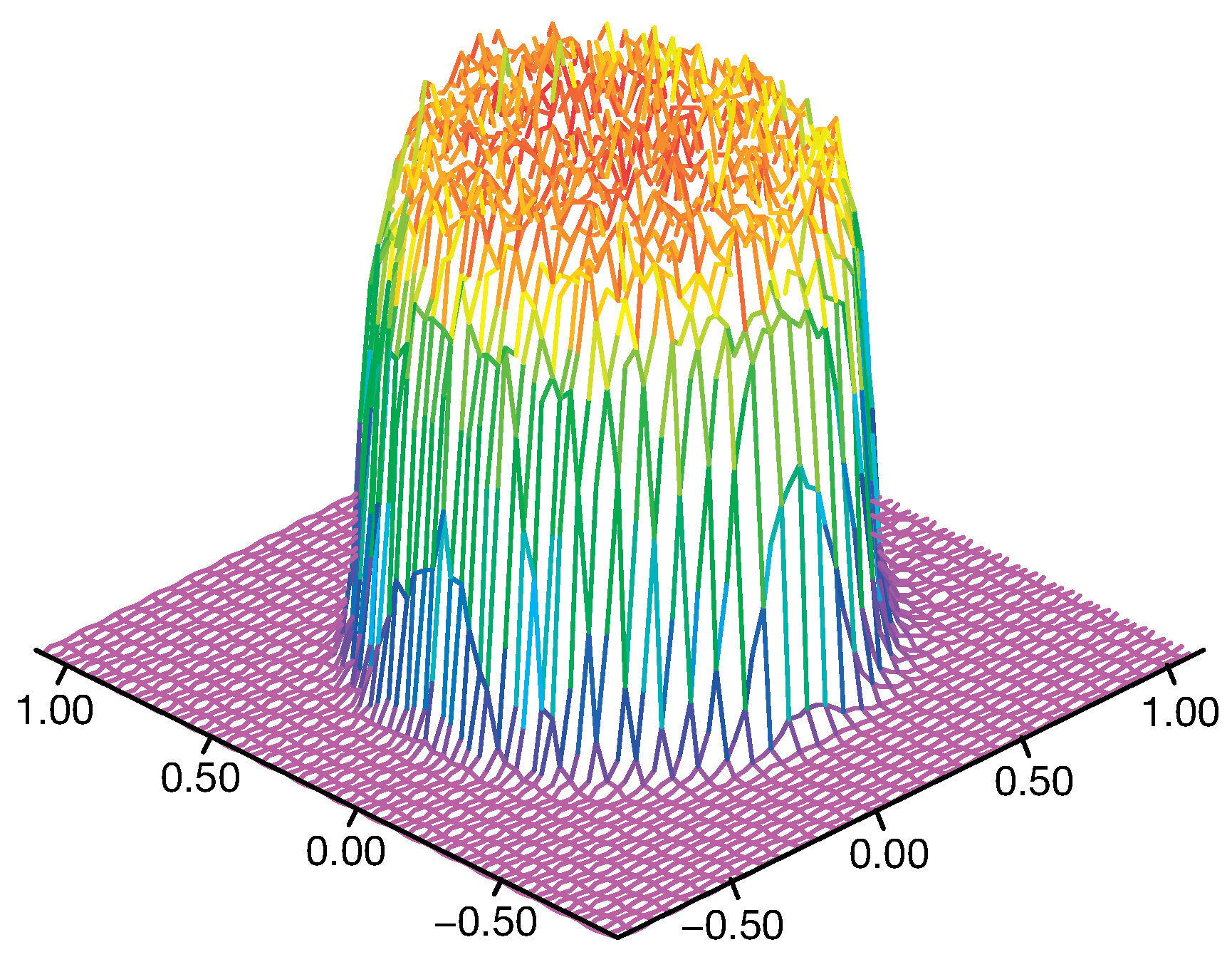
3.2. Energy Source
3.3. Addition of Deposited Material
4. FE Implementation of the Hybrid Model
- Fourteen deposition tests (regression sample) were used to fit the regression models used to identify the analytic models required to control the activation strategy implemented in the UEPACTIVATIONVOL user-defined subroutine;
- Six deposition tests (regression validation sample) were used to validate the regression models previously identified;
- Seven deposition tests (FE validation sample, Table 2), with increasing laser power (P), powder feed rate (Q), and scanning speed (v) values, were extracted in order to validate the FE model.
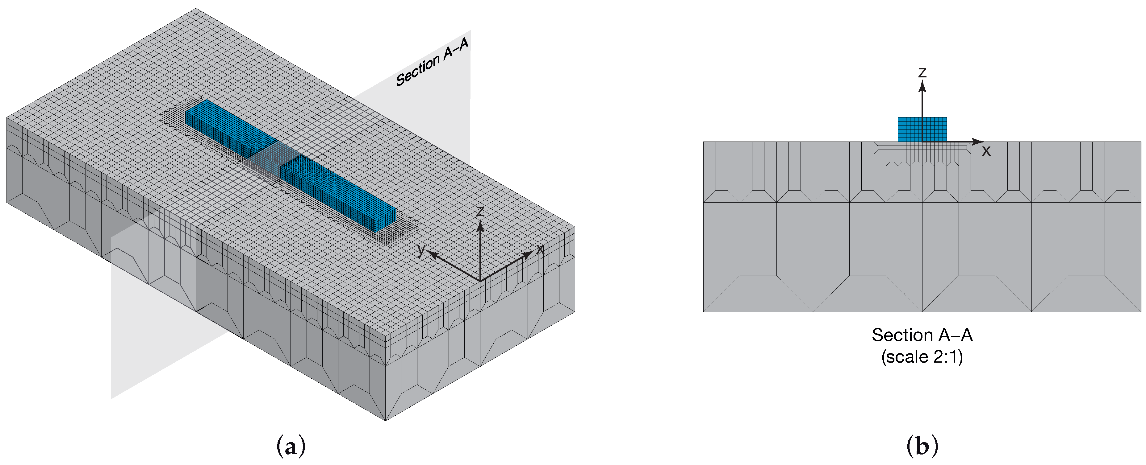
4.1. Geometry and Mesh
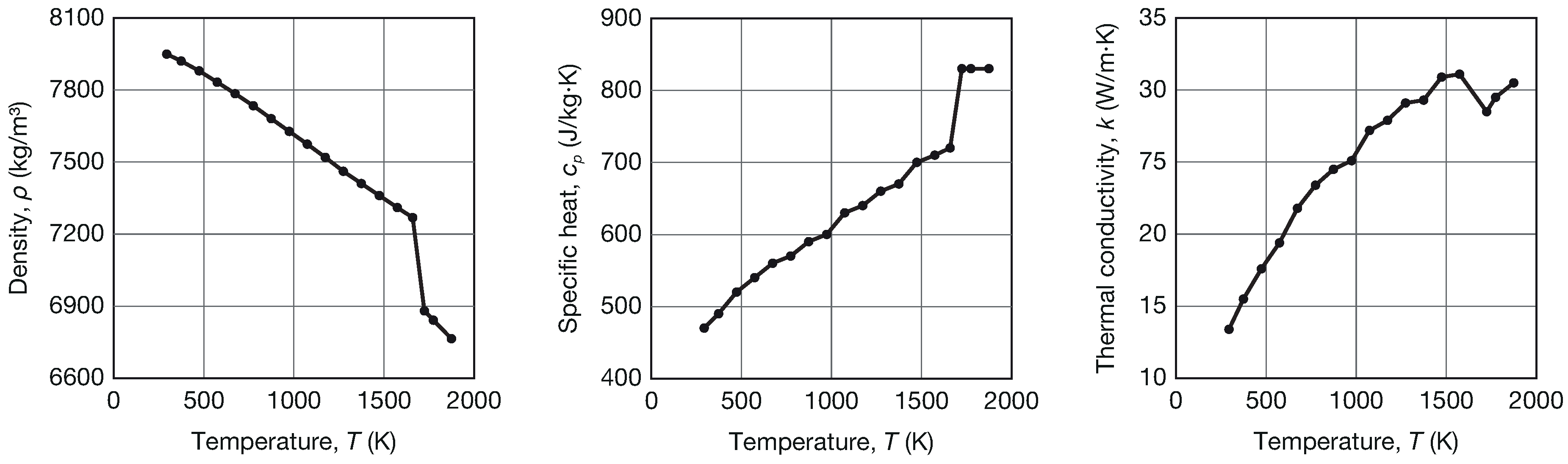
4.2. Material Properties
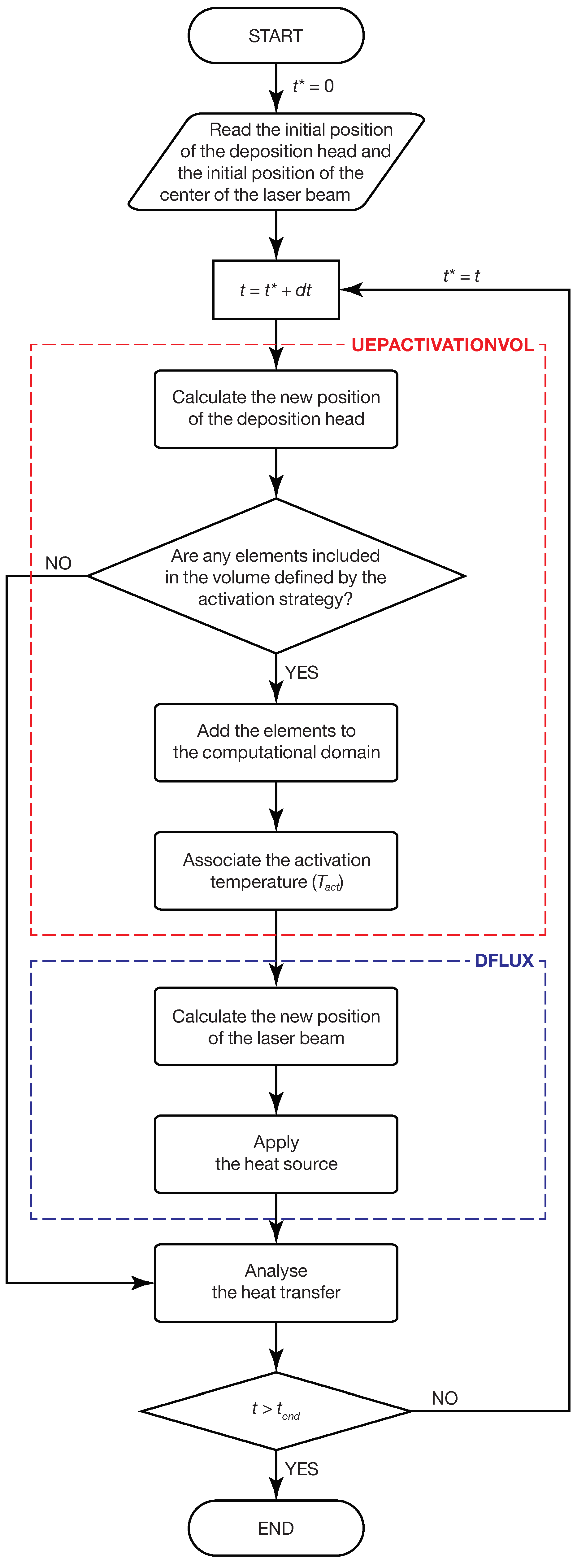
4.3. Activation Strategy
5. Results and Discussion
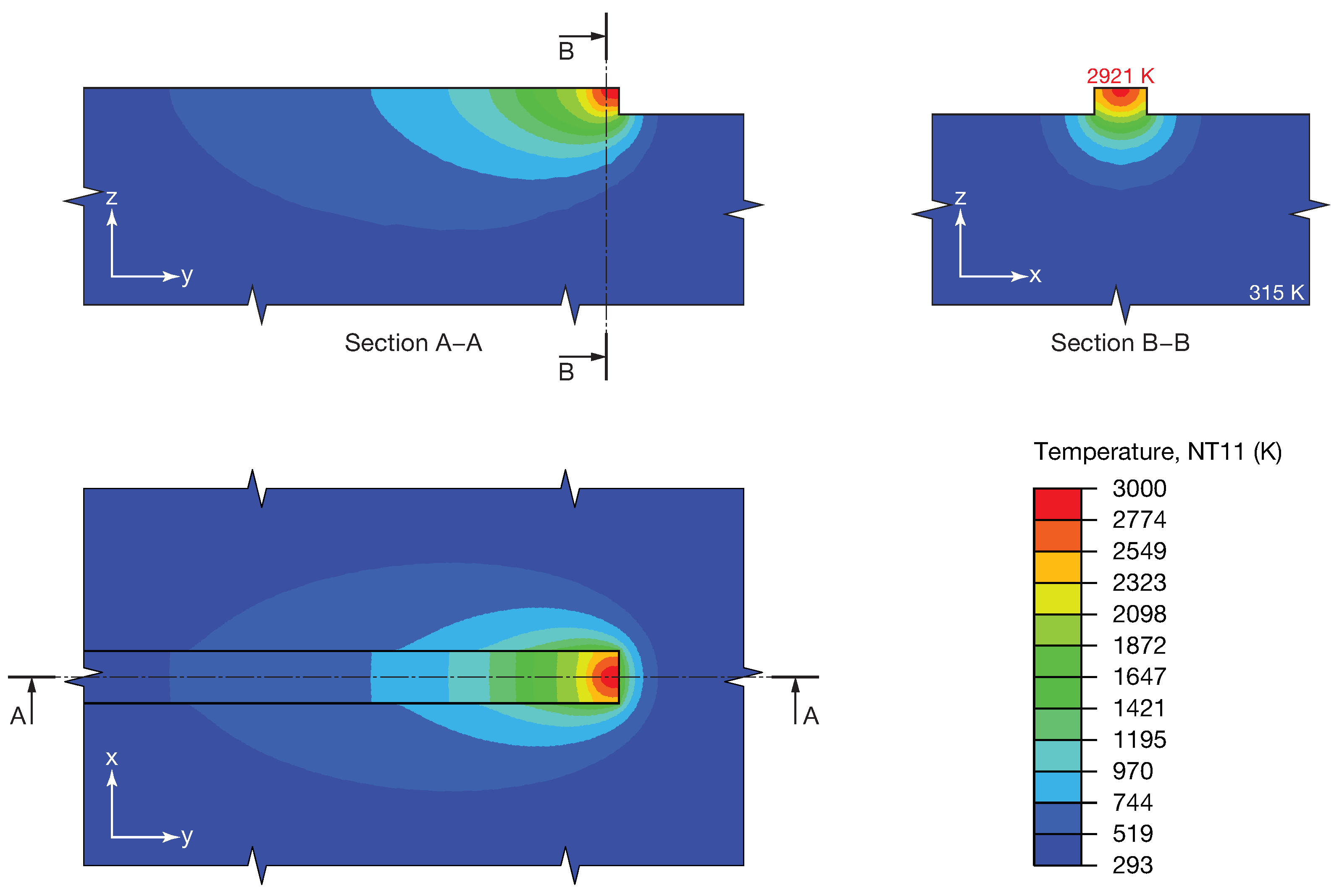
5.1. Temperature Distribution
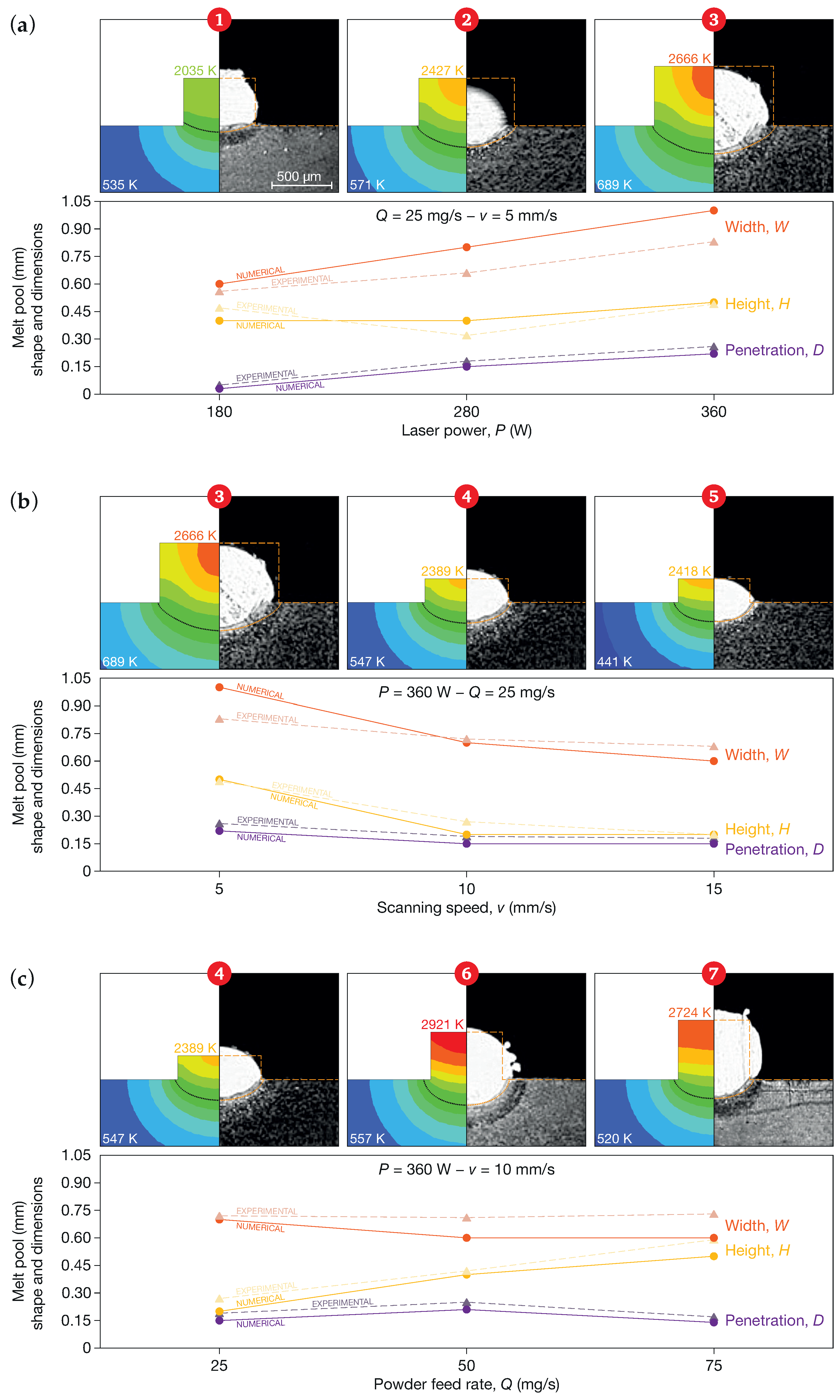
5.2. Melt Pool Shape and Dimensions
6. Conclusions
- a novel material addition strategy was adopted, in which the volume of the deposited material was a function of process parameters and was modeled by combining regression-based analytic models with an element activation approach in the Abaqus software tool;
- a comparison with experimental data from the literature showed that the the model was able to predict the height and the width of the deposited track with an average percentage error of 14% and a maximum deviation of , as well as the penetration depth with an average percentage error of 18% and a maximum deviation of ; the forecasting accuracy was consistent with the adopted mesh resolution;
- by comparing the proposed model with other models available in the literature, the prediction error was slightly higher, being approximately 10%, the typical declared error for the track height; as concerns the track width, the prediction error was within the variability of actual tracks;
- the model was thus able to capture the main aspects of the process physics and to make a reasonable short-time forecast of the results, in terms of track geometry and temperatures;
- the model allowed recognizing whether a set of process parameters would ensure adhesion between the deposited material and the substrate; this allowed the limits of the process parameter window to be identified, and thus saving time and the cost of a complete experimental campaign.
Author Contributions
Funding
Acknowledgments
Conflicts of Interest
Appendix A. Source Code Listing of User-Defined Subroutines in Abaqus
Appendix A.1. UEPACTIVATIONVOL User-Defined Subroutine

Appendix A.2. DFLUX User-Defined Subroutine

References
- Frazier, W.E. Metal Additive Manufacturing: A Review. J. Mater. Eng. Perform. 2014, 23, 1917–1928. [Google Scholar] [CrossRef]
- Calignano, F.; Manfredi, D.; Ambrosio, E.P.; Biamino, S.; Lombardi, M.; Atzeni, E.; Salmi, A.; Minetola, P.; Iuliano, L.; Fino, P. Overview on Additive Manufacturing Technologies. Proc. IEEE 2017, 105, 593–612. [Google Scholar] [CrossRef]
- Gu, D.D.; Meiners, W.; Wissenbach, K.; Poprawe, R. Laser additive manufacturing of metallic components: Materials, processes and mechanisms. Int. Mater. Rev. 2013, 57, 133–164. [Google Scholar] [CrossRef]
- Thompson, M.K.; Moroni, G.; Vaneker, T.; Fadel, G.; Campbell, R.I.; Gibson, I.; Bernard, A.; Schulz, J.; Graf, P.; Ahuja, B.; et al. Design for Additive Manufacturing: Trends, opportunities, considerations, and constraints. CIRP Ann. 2016, 65, 737–760. [Google Scholar] [CrossRef]
- Gibson, I.; Rosen, D.W.; Stucker, B. Design for Additive Manufacturing. In Additive Manufacturing Technologies; Springer: New York, NY, USA, 2010; Book Section Chapter 11; pp. 299–332. [Google Scholar] [CrossRef]
- Wohlers Associates. Wohlers Report 2018: 3D Printing and Additive Manufacturing State of the Industry; Annual Worldwide Progress Report; Wohlers Associates, Inc.: Fort Collins, CO, USA, 2018. [Google Scholar]
- Thompson, S.M.; Bian, L.; Shamsaei, N.; Yadollahi, A. An overview of Direct Laser Deposition for additive manufacturing; Part I: Transport phenomena, modeling and diagnostics. Addit. Manuf. 2015, 8, 36–62. [Google Scholar] [CrossRef]
- Pinkerton, A.J. Advances in the modeling of laser direct metal deposition. J. Laser Appl. 2015, 27. [Google Scholar] [CrossRef]
- Mazumder, J.; Dutta, D.; Kikuchi, N.; Ghosh, A. Closed loop direct metal deposition: Art to part. Opt. Lasers Eng. 2000, 34, 397–414. [Google Scholar] [CrossRef]
- Toyserkani, E.; Khajepour, A.; Corbin, S. Laser Cladding; CRC Press: Boca Raton, FL, USA, 2005. [Google Scholar]
- Zhang, Y.; Chen, Q.; Guillemot, G.; Gandin, C.A.; Bellet, M. Numerical modeling of fluid and solid thermomechanics in additive manufacturing by powder-bed fusion: Continuum and level set formulation applied to track- and part-scale simulations. Comptes Rendus Mécanique 2018, 346, 1055–1071. [Google Scholar] [CrossRef]
- Megahed, M.; Mindt, H.W.; N’Dri, N.; Duan, H.; Desmaison, O. Metal additive-manufacturing process and residual stress modeling. Integr. Mater. Manuf. Innov. 2016, 5, 61–93. [Google Scholar] [CrossRef] [Green Version]
- Vilar, R. 10.07—Laser Powder Deposition. In Comprehensive Materials Processing; Elsevier: Amsterdam, The Netherlands, 2014; pp. 163–216. [Google Scholar] [CrossRef]
- Ahsan, M.N.; Pinkerton, A.J. An analytical-numerical model of laser direct metal deposition track and microstructure formation. Model. Simul. Mater. Sci. Eng. 2011, 19. [Google Scholar] [CrossRef]
- Pinkerton, A.J. Laser direct metal deposition: Theory and applications in manufacturing and maintenance. In Advances in Laser Materials Processing; Elsevier: Amsterdam, The Netherlands, 2010; pp. 461–491. [Google Scholar]
- Gibson, I.; Rosen, D.; Stucker, B. Directed Energy Deposition Processes. In Additive Manufacturing Technologies; Springer: New York, NY, USA, 2015; Chapter 10; pp. 245–268. [Google Scholar] [CrossRef]
- Pinkerton, A.J.; Li, L. Modelling Powder Concentration Distribution From a Coaxial Deposition Nozzle for Laser-Based Rapid Tooling. J. Manuf. Sci. Eng. 2004, 126. [Google Scholar] [CrossRef]
- Ibarra-Medina, J.; Pinkerton, A.J. Numerical investigation of powder heating in coaxial laser metal deposition. Surf. Eng. 2013, 27, 754–761. [Google Scholar] [CrossRef]
- Lin, J. Laser attenuation of the focused powder streams in coaxial laser cladding. J. Laser Appl. 2000, 12, 28–33. [Google Scholar] [CrossRef]
- Unocic, R.R.; DuPont, J.N. Process efficiency measurements in the laser engineered net shaping process. Metall. Mater. Trans. B 2004, 35, 143–152. [Google Scholar] [CrossRef]
- Qi, H.; Mazumder, J.; Ki, H. Numerical simulation of heat transfer and fluid flow in coaxial laser cladding process for direct metal deposition. J. Appl. Phys. 2006, 100. [Google Scholar] [CrossRef]
- Gan, Z.; Yu, G.; He, X.; Li, S. Numerical simulation of thermal behavior and multicomponent mass transfer in direct laser deposition of Co-base alloy on steel. Int. J. Heat Mass Transf. 2017, 104, 28–38. [Google Scholar] [CrossRef] [Green Version]
- Lee, Y.; Nordin, M.; Babu, S.; Farson, D. Influence of fluid convection on weld pool formation in laser cladding. Weld. J. 2014, 93, 292s–300s. [Google Scholar]
- Manvatkar, V.; De, A.; DebRoy, T. Heat transfer and material flow during laser assisted multi-layer additive manufacturing. J. Appl. Phys. 2014, 116. [Google Scholar] [CrossRef]
- Hofmeister, W.; Wert, M.; Smugeresky, J.; Philliber, J.A.; Griffith, M.; Ensz, M. Investigating solidification with the laser-engineered net shaping (LENSTM) process. JOM 1999, 51, 1–6. [Google Scholar]
- Hu, D.; Kovacevic, R. Modelling and measuring the thermal behavior of the molten pool in closed-loop controlled laser-based additive manufacturing. Proc. Inst. Mech. Eng. Part B J. Eng. Manuf. 2005, 217, 441–452. [Google Scholar] [CrossRef]
- Vinokurov, V.A. Welding Stresses and Distortion: Determination and Elimination; British Library Lending Division: Boston Spa, UK, 1977. [Google Scholar]
- Brown, S.; Song, H. Finite Element Simulation of Welding of Large Structures. J. Eng. Ind. 1992, 114, 441–451. [Google Scholar] [CrossRef]
- Labudovic, M.; Hu, D.; Kovacevic, R. A three dimensional model for direct laser metal powder deposition and rapid prototyping. J. Mater. Sci. 2003, 38, 35–49. [Google Scholar] [CrossRef]
- Toyserkani, E.; Khajepour, A.; Corbin, S. Three-dimensional finite element modeling of laser cladding by powder injection: Effects of powder feedrate and travel speed on the process. J. Laser Appl. 2003, 15, 153–160. [Google Scholar] [CrossRef]
- Toyserkani, E.; Khajepour, A.; Corbin, S. 3-D finite element modeling of laser cladding by powder injection: effects of laser pulse shaping on the process. Opt. Lasers Eng. 2004, 41, 849–867. [Google Scholar] [CrossRef]
- Costa, L.; Vilar, R.; Reti, T.; Deus, A.M. Rapid tooling by laser powder deposition: Process simulation using finite element analysis. Acta Mater. 2005, 53, 3987–3999. [Google Scholar] [CrossRef]
- Wang, L.; Felicelli, S.; Gooroochurn, Y.; Wang, P.; Horstemeyer, M. Numerical Simulation of the Temperature Distribution and Solidphase Evolution in the LENS™ Process. In Proceedings of the Seventeenth Solid Freeform Fabrication Symposium, Austin, TX, USA, 14–16 August 2006. [Google Scholar]
- Peyre, P.; Aubry, P.; Fabbro, R.; Neveu, R.; Longuet, A. Analytical and numerical modeling of the direct metal deposition laser process. J. Phys. D Appl. Phys. 2008, 41. [Google Scholar] [CrossRef]
- Fallah, V.; Alimardani, M.; Corbin, S.F.; Khajepour, A. Temporal development of melt-pool morphology and clad geometry in laser powder deposition. Comput. Mater. Sci. 2011, 50, 2124–2134. [Google Scholar] [CrossRef]
- Neela, V.; De, A. Three-dimensional heat transfer analysis of LENSTM process using finite element method. Int. J. Adv. Manuf. Technol. 2009, 45, 935–943. [Google Scholar] [CrossRef]
- Manvatkar, V.D.; Gokhale, A.A.; Jagan Reddy, G.; Venkataramana, A.; De, A. Estimation of Melt Pool Dimensions, Thermal Cycle, and Hardness Distribution in the Laser-Engineered Net Shaping Process of Austenitic Stainless Steel. Metall. Mater. Trans. A 2011, 42, 4080–4087. [Google Scholar] [CrossRef]
- Amine, T.; Newkirk, J.W.; Liou, F. Investigation of effect of process parameters on multilayer builds by direct metal deposition. Appl. Therm. Eng. 2014, 73, 500–511. [Google Scholar] [CrossRef]
- Chiumenti, M.; Lin, X.; Cervera, M.; Lei, W.; Zheng, Y.; Huang, W. Numerical simulation and experimental calibration of additive manufacturing by blown powder technology. Part I: Thermal analysis. Rapid Prototyp. J. 2017, 23, 448–463. [Google Scholar] [CrossRef]
- Shah, K.; Khurshid, H.; ul Haq, I.; Anwar, S.; Shah, S.A. Numerical modeling of pulsed and continuous wave direct laser deposition of Ti-6Al-4V and Inconel 718. Int. J. Adv. Manuf. Technol. 2017, 95, 847–860. [Google Scholar] [CrossRef]
- Michaleris, P. Modeling metal deposition in heat transfer analyses of additive manufacturing processes. Finite Elem. Anal. Des. 2014, 86, 51–60. [Google Scholar] [CrossRef]
- Fang, H.Y.; Wang, T.; Hu, J.F.; Yang, J.G. Node dynamic relaxation method: Principle and application. Front. Mater. Sci. 2011, 5, 179–195. [Google Scholar] [CrossRef]
- Lampa, C.; Kaplan, A.F.H.; Powell, J.; Magnusson, C. An analytical thermodynamic model of laser welding. J. Phys. D Appl. Phys. 1997, 30, 1293–1299. [Google Scholar] [CrossRef]
- Gouge, M.F.; Heigel, J.C.; Michaleris, P.; Palmer, T.A. Modeling forced convection in the thermal simulation of laser cladding processes. Int. J. Adv. Manuf. Technol. 2015, 79, 307–320. [Google Scholar] [CrossRef]
- Yang, Q.; Zhang, P.; Cheng, L.; Min, Z.; Chyu, M.; To, A.C. Finite element modeling and validation of thermomechanical behavior of Ti-6Al-4V in directed energy deposition additive manufacturing. Addit. Manuf. 2016, 12, 169–177. [Google Scholar] [CrossRef]
- Heigel, J.C.; Michaleris, P.; Reutzel, E.W. Thermo-mechanical model development and validation of directed energy deposition additive manufacturing of Ti-6Al-4V. Addit. Manuf. 2015, 5, 9–19. [Google Scholar] [CrossRef]
- Goldak, J.; Chakravarti, A.; Bibby, M. A new finite element model for welding heat sources. Metall. Trans. B 1984, 15, 299–305. [Google Scholar] [CrossRef]
- El Cheikh, H.; Courant, B.; Branchu, S.; Hascoët, J.Y.; Guillén, R. Analysis and prediction of single laser tracks geometrical characteristics in coaxial laser cladding process. Opt. Lasers Eng. 2012, 50, 413–422. [Google Scholar] [CrossRef] [Green Version]
- Picasso, M.; Marsden, C.F.; Wagniere, J.D.; Frenk, A.; Rappaz, M. A simple but realistic model for laser cladding. Metall. Mater. Trans. B 1994, 25, 281–291. [Google Scholar] [CrossRef]
- Huang, Y.L.; Liu, J.; Ma, N.H.; Li, J.G. Three-dimensional analytical model on laser-powder interaction during laser cladding. J. Laser Appl. 2006, 18, 42–46. [Google Scholar] [CrossRef]
- Diniz Neto, O.O.; Alcalde, A.M.; Vilar, R. Interaction of a focused laser beam and a coaxial powder jet in laser surface processing. J. Laser Appl. 2007, 19, 84–88. [Google Scholar] [CrossRef]
- Ibarra-Medina, J.; Pinkerton, A.J. A CFD model of the laser, coaxial powder stream and substrate interaction in laser cladding. Phys. Procedia 2010, 5, 337–346. [Google Scholar] [CrossRef]
- He, X.; Mazumder, J. Transport phenomena during direct metal deposition. J. Appl. Phys. 2007, 101. [Google Scholar] [CrossRef]
- Wen, S.Y.; Shin, Y.C.; Murthy, J.Y.; Sojka, P.E. Modeling of coaxial powder flow for the laser direct deposition process. Int. J. Heat Mass Transf. 2009, 52, 5867–5877. [Google Scholar] [CrossRef]
- Huang, Y.; Khamesee, M.B.; Toyserkani, E. A comprehensive analytical model for laser powder-fed additive manufacturing. Addit. Manuf. 2016, 12, 90–99. [Google Scholar] [CrossRef]
- Jiazhu, W.; Liu, T.; Chen, H.; Li, F.; Wei, H.; Zhang, Y. Simulation of laser attenuation and heat transport during direct metal deposition considering beam profile. J. Mater. Process. Technol. 2019, 270, 92–105. [Google Scholar] [CrossRef]
- Mills, K.C. Recommended Values of Thermophysical Properties for Selected Commercial Alloys; Woodhead Publishing, Elsevier: Sawston, UK; Cambridge, UK, 2002; p. ix. 244p. [Google Scholar]
- Touloukian, Y.; DeWitt, D. Thermophysical Properties of Matter—The TPRC Data Series. Volume 8. Thermal Radiative Properties—Nonmetallic Solids. (Reannouncement). Data Book; Report AD-A-951942/2/XAB; Other: CNN: DSA900-73-C-2101 United States Other: CNN: DSA900-73-C-2101 NTIS GRA English; Thermophysical and Electronic Properties Information Center, Purdue Univ: Lafayette, IN, USA, 1972. [Google Scholar]
- Caiazzo, F.; Alfieri, V.; Argenio, P.; Sergi, V. Additive manufacturing by means of laser-aided directed metal deposition of 2024 aluminium powder: Investigation and optimization. Adv. Mech. Eng. 2017, 9. [Google Scholar] [CrossRef]
- Caiazzo, F.; Caggiano, A. Laser Direct Metal Deposition of 2024 Al Alloy: Trace Geometry Prediction via Machine Learning. Materials 2018, 11, 444. [Google Scholar] [CrossRef]


| Ref. | Materials | Model Output | Assumptions |
|---|---|---|---|
| [25] | 316L | Temperature distribution | No heat source No convection or radiation Substrate at a constant temperature Elements activated at the melting temperature |
| [26] | Mild steel | Melt pool dimensions | Gaussian distribution of the heat source Latent heat included by a modification of the specific heat Combined heat transfer coefficient No Marangoni flows The addition of material is neglected |
| [29] | 400 Monel alloy | Temperature distribution Melt pool dimensions Residual stress distribution | Gaussian distribution of the heat source Latent heat included by a modification of the specific heat Combined heat transfer coefficient No Marangoni flows |
| [30] | Iron | Effect of laser pulsed shape parameters on the geometryof the deposited material | Gaussian distribution of the heat sourceLatent heat included by a modification of the specific heat
Combined heat transfer coefficient |
| [31] | Iron | Effect of powder feed rate and scanning speed on the geometryof the deposited material | Gaussian distribution of the heat source Latent heat included by a modification of the specific heat
Combined heat transfer coefficient |
| [32] | 420 steel | Microstructure Hardness | Gaussian distribution of the heat source Convection coefficient = 30 /() An internal heat source simulates the latent heat Elements activated at their melting temperature |
| [33] | SS410 | Solid phase evolution | Gaussian distribution of the heat source |
| [34] | Ti-6Al-4V | Temperature distribution in the substrate | Heat source applied to the substrate Convection coefficient = 20 /() Addition of material simulated by a modification of the thermal conductivity |
| [35] | 304 L | Track geometry Temperature distribution in the substrate | Gaussian distribution of the heat source Latent heat included by a modification of the specific heat Heat source applied to the substrate Convection coefficient = 40 /() Elements activated at ambient temperature |
| [36] | SS316 | Temperature distribution | Gaussian distribution of the heat source Convection coefficient = 10 /() Initial temperature of the entire model = 300 |
| [14] | Ti-6Al-4 V | Temperature distribution | Track geometry No radiation or convection Gaussian distribution of the heat source No Marangoni flows |
| [37] | 316L | Peak temperature/cooling rate Melt pool geometry | Gaussian distribution of the heat source No radiation |
| [38] | 316L | Temperature distribution Re-melted depth | Natural convection Gaussian distribution of the heat source |
| [39] | Ti-6Al-4V | Temperature distribution in the substrate | Combined heat transfer coefficient Heat source applied as a constant energy density Model calibration is required |
| [40] | Ti-6Al-4V Inconel 718 | Residual stress distribution | Rectangular laser beam shape No radiation Convection coefficient = 20 /() No Marangoni flows |
| [22] | Co-base alloy | Temperature distribution | Gaussian distribution of the heat source No energy attenuation Convection coefficient = 100 /() |
| Set | P | Q | v |
|---|---|---|---|
| () | (/) | (/) | |
| 1 | 180 | 25 | 5 |
| 2 | 280 | 25 | 5 |
| 3 | 360 | 25 | 5 |
| 4 | 360 | 25 | 10 |
| 5 | 360 | 25 | 15 |
| 6 | 360 | 50 | 10 |
| 7 | 360 | 75 | 10 |
| Property | Value |
|---|---|
| Solidus temperature, | 1674 |
| Liquidus temperature, | 1697 |
| Latent heat of fusion, | / |
| Surface emissivity coefficient, | 0.6 |
| P | Q | v | ||||||||
|---|---|---|---|---|---|---|---|---|---|---|
| () | (/) | (/) | (mm) | (mm) | (mm) | (%) | (mm) | (mm) | (mm) | (%) |
| 180 | 75 | 10 | 0.47 | 0.45 | -0.02 | −5% | 0.39 | 0.43 | +0.04 | 9% |
| 280 | 50 | 10 | 0.37 | 0.35 | -0.02 | −5% | 0.62 | 0.56 | -0.06 | −10% |
| 280 | 75 | 5 | 0.80 | 0.93 | +0.13 | 16% | 0.65 | 0.67 | +0.02 | 3% |
| 280 | 75 | 15 | 0.27 | 0.32 | +0.05 | 20% | 0.56 | 0.47 | -0.09 | −16% |
| 360 | 50 | 5 | 0.82 | 0.72 | -0.10 | −12% | 0.86 | 0.89 | +0.03 | 4% |
| 360 | 50 | 15 | 0.26 | 0.26 | +0.00 | 0% | 0.62 | 0.55 | -0.07 | −12% |
| Set | ||||||||||||
|---|---|---|---|---|---|---|---|---|---|---|---|---|
| (mm) | (mm) | (mm) | (%) | (mm) | (mm) | (mm) | (%) | (mm) | (mm) | (mm) | (%) | |
| 1 | 0.47 | 0.40 | -0.07 | −15% | 0.56 | 0.60 | 0.04 | 7% | 0.03 | 0.05 | 0.02 † | 67% † |
| 2 | 0.32 | 0.40 | 0.08 | 25% | 0.66 | 0.80 | 0.14 | 21% | 0.15 | 0.18 | 0.03 | 20% |
| 3 | 0.49 | 0.50 | 0.01 | 2% | 0.83 | 1.00 | 0.17 | 20% | 0.22 | 0.26 | 0.04 | 18% |
| 4 | 0.27 | 0.20 | -0.07 | −26% | 0.72 | 0.70 | -0.02 | −3% | 0.15 | 0.19 | 0.04 | 27% |
| 5 | 0.20 | 0.20 | 0.00 | 0% | 0.68 | 0.60 | -0.08 | −12% | 0.15 | 0.18 | 0.03 | 20% |
| 6 | 0.42 | 0.40 | -0.02 | −5% | 0.71 | 0.60 | -0.11 | −15% | 0.21 | 0.25 | 0.04 | 19% |
| 7 | 0.59 | 0.50 | -0.09 | −15% | 0.73 | 0.60 | -0.13 | −18% | 0.14 | 0.17 | 0.03 | 21% |
© 2019 by the authors. Licensee MDPI, Basel, Switzerland. This article is an open access article distributed under the terms and conditions of the Creative Commons Attribution (CC BY) license (http://creativecommons.org/licenses/by/4.0/).
Share and Cite
Piscopo, G.; Atzeni, E.; Salmi, A. A Hybrid Modeling of the Physics-Driven Evolution of Material Addition and Track Generation in Laser Powder Directed Energy Deposition. Materials 2019, 12, 2819. https://doi.org/10.3390/ma12172819
Piscopo G, Atzeni E, Salmi A. A Hybrid Modeling of the Physics-Driven Evolution of Material Addition and Track Generation in Laser Powder Directed Energy Deposition. Materials. 2019; 12(17):2819. https://doi.org/10.3390/ma12172819
Chicago/Turabian StylePiscopo, Gabriele, Eleonora Atzeni, and Alessandro Salmi. 2019. "A Hybrid Modeling of the Physics-Driven Evolution of Material Addition and Track Generation in Laser Powder Directed Energy Deposition" Materials 12, no. 17: 2819. https://doi.org/10.3390/ma12172819