Article

Robust Longitudinal Speed Control of Hybrid Electric Vehicles with a Two-Degree-of-Freedom Fuzzy Logic Controller

Department of Mechanical and Electro-Mechanical Engineering, National Sun Yat-Sen University, Kaohsiung 80424, Taiwan
*
Author to whom correspondence should be addressed.
Energies 2016, 9(4), 290; https://doi.org/10.3390/en9040290
Submission received: 6 January 2016 / Revised: 30 March 2016 / Accepted: 7 April 2016 / Published: 16 April 2016
(This article belongs to the Special Issue Power Management for Hybrids and Vehicle Drivetrains)

Abstract

:
This paper proposes a new robust two-degree-of-freedom (DoF) design method for controlling the nonlinear longitudinal speed problem of hybrid electric vehicles (HEVs). First, the uncertain parameters of the HEV model are described by fuzzy α-cut representation, in which the interval uncertainty and the possibility can be simultaneously indicated by the fuzzy membership function. For the fuzzy parametric uncertain system, the maximum uncertainty interval can be translated into the weighting matrix Q of the linear quadratic tracking problem to guarantee that the designed feedback controller is robust. Second, the fuzzy forward compensator is incorporated with a robust feedback controller to enhance the system tracking response. The simulation results demonstrate that the proposed controller has higher tracking performance compared to the single-DoF self-tuning fuzzy logic controller or conventional optimal H controller.

1. Introduction

Recently, increasing concern about a cleaner environment and fuel conservation has made hybrid electric vehicles (HEVs) an indispensable next-generation technology. HEVs coordinate both electric machines and internal combustion engines (ICEs) to deliver propulsion power. Many previous studies have focused on the energy management and optimal power flow of HEV dynamics [1,2,3,4]. However, HEV speed control techniques are drastically different than those of a conventional vehicle, because HEVs typically move in electric mode, and ICEs can be operated at higher speeds. Therefore, the drive performance and wide-range speed control algorithm of HEVs are also key concerns [5]. The practical application of speed control includes adaptive cruise control, intelligent collision avoidance and car following [6,7,8].
In the traditional ICE propulsion system, the vehicle speed and engine power are directly controlled by the mechanical throttle control system (MTCS). However, the hybrid powertrain request does not go directly to the engine in HEVs; instead, the MTCS is replaced by an electronic throttle control system (ETCS) [9,10,11]. The ETCS system is a complex engine mechanism that utilizes a DC servo motor to regulate the throttle position. With ETCS, the desired torque and a wide range of vehicle speeds can be achieved in HEVs [12]. In addition, HEV speed control must combine ETCS with nonlinear vehicle dynamics. Because of factors such as the uncertainty parameters of nonlinear elements and instability from environmental disturbances, designing an algorithm for HEV speed control is challenging [13].
Longitudinal speed control belongs to a group of wide-range and cyclic operations. The goal of HEV speed response is to track a desired speed under any operating condition. A robust and adaptive internal model control algorithm was used to track speed and reject road grade disturbance in [14]. The sliding mode control, incorporated with an adaptive proportional-integral-derivative (PID) controller, was proposed to solve the uncertain speed servo problem [15]. The speed control performance among the state feedback controller, intelligent control techniques and adaptive controller was compared in [16]. However, these previous studies have two limitations. First, the uncertainty of the dynamic system model can generally be described as a bounded interval model that considers each operational point with equal probability. Compared to the interval approach, the fuzzy α -cut representation of uncertainties can use the fuzzy membership function to indicate the possibilities and intervals of variations. Such a fuzzy parametric uncertain system (FPUS) can be viewed as an extension of interval systems and has attracted considerable attention from researchers [17,18,19]. In [20], the problem of designing a robust controller for FPUS was converted into an optimal linear quadratic regulator (LQR) control approach. The optimal LQR controller, which was designed for the worst-case condition ( α = 0 ) , can stabilize all systems for various values of α [ 0 , 1 ] . Second, previous studies have addressed control schemes in one-degree-of-freedom (1-DoF) controllers, which may address them for specific types of performance, but be compromised in others. Two-degree-of-freedom (2-DoF) controllers can fulfill another performance requirement by adding a feed-forward controller or prefilter. For example, combining a forward fuzzy prefilter and a feedback controller for hydraulically-actuated robotic mechanisms was studied in [21]. Because the prefilter can compensate the effects of the dead-zone of the electromagnetic proportional control valve, the 2-DoF controller has quite good tracking trajectories compared to the conventional 1-DoF controller. In [22], the 2-DoF integral-P (IP) controller for electrical drives was shown to have good reference tracking and load-torque rejection performance. Coordinating the inner loop observer to reject disturbances and an outer loop tracking controller to achieve control performances was successful implemented in robust yaw stability control of electric vehicles [23]. Therefore, 2-DoF control systems can be used to enhance wide-range operations.
This paper investigates the nonlinear longitudinal speed control model of HEVs with fuzzy parametric uncertain systems and proposes a new robust 2-DoF design method of speed control systems for HEVs. The design procedure consists of two steps. In the first step, the different loads of HEV components are described according to a fuzzy α -cut number, and the maximum uncertainty interval of the system is translated into the weighting matrix Q of the linear quadratic tracking (LQT) servo problem, to guarantee that the designed feedback optimal controller is robust under the worst-case condition. In the second step, a fuzzy forward compensator is incorporated with a robust feedback controller to enhance the system response. The robust property of the proposed controller can track a desired speed at a wide range of vehicle speeds with varying road grades. In addition, the fast dynamic response has significant effects on engine performance, fuel consumption and pollution emission, especially in the transition mode of the hybrid operating system of HEVs. The effectiveness of this longitudinal speed controller has been demonstrated in simulation studies.
The remainder of this paper is organized as follows. Section 2 details the fuzzy parametric uncertain system for HEV speed control. In Section 3, the methodology for the synthesis of the 2-DoF fuzzy controller and the stability analysis of the proposed controller are presented. The simulation implementation of the proposed controller, with other controllers, such as the H and 1-DoF self-tuning fuzzy PID controllers, are described in Section 4. Finally, Section 5 presents the conclusions of this study.

2. Problem Formulation and Longitudinal Speed Control Modeling

This paper focuses on the speed control of a small HEV with an uncertain parameter of ETCS and a nonlinear vehicle dynamic model, the control scheme for which is shown in Figure 1. The uncertainty component parameters are listed in Table 1 [12].

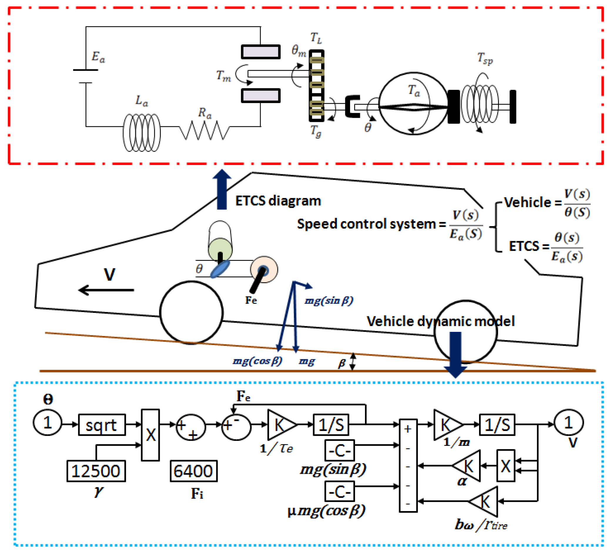
2.1. The Architecture of the HEV Model

The speed control architecture of the HEV includes an engine with ETCS and a nonlinear vehicle longitudinal motion model. The ETCS uses a DC servo motor to adjust the throttle, as expressed in the governing differential Equations (1)–(3) [9].
d i a d t = 1 L a ( R a i a K b d θ m d t + E a )
d 2 θ m d t 2 = 1 J m ( B m d θ m d t T L + T m )
d 2 θ d t 2 = 1 J g ( T s p B t d θ d t T a + T g )
where i a is armature current (A), T s p is the spring torque and θ m and θ are the angular position (rad) of the armature and throttle plate, respectively. R a and L a represent the armature resistance and inductance, respectively. The back electromotive force constant is K b . The parameters B m and B t are defined as the motor shaft and throttle viscous damping coefficients, respectively. T a is the torque due to airflow. Motor inertia and throttle inertia are defined as J m and J g , respectively. Assume the gear ratio N and the motor torque T m can be expanded as:
N = θ m θ = T g T L
T m = K t i a
where T g is the torque transmitted from gears, T L is the load torque and K t is motor torque constant.
Equations (1) and (2) can be expressed in terms of throttle plate angular rotation as:
d i a d t = 1 L a ( R a i a K b N d θ d t + E a )
d 2 θ d t 2 = 1 N 2 J m + J g ( T s p ( N 2 B m + B t ) d θ d t T a + N T m )
For simplicity, let spring torque T s p = 2 K s p × θ , equivalent inertia J = N 2 J m + J g and damping constant B = N 2 B m + B t . Taking the Laplace transform of Equations (6) and (7) into the s-domain, we obtain:
θ ( s ) E a ( s ) = N K t / L a J s 3 + R a J + B L a L a J s 2 + R a B + N 2 K t K b + 2 K s p L a L a J s + 2 K s p R a L a J
From Table 1, the nominal transfer function of ETCS is given as:
θ ( s ) E a ( S ) = 6349 s 3 + 689.7 s 2 + 1.82 × 10 4 s + 2.54 × 10 4
The dynamics of the nonlinear HEVs is given as [12,16]:
m d V d t = F i + γ θ τ e d F e ( θ ) d t μ m g ( c o s β ) α V 2 b ω V r t i r e m g ( s i n β )
where F i and F e are the engine idle force and engine force. γ , μ , α and b ω are the coefficients of engine force, friction, drag and bearing damping, respectively. τ e is the engine time constant. β is the road slope.
The Simulink model of the nonlinear vehicle dynamic Equation (10) is depicted in Figure 1. The procedure of linearization of the nominal model [12] is as follows: First, β = 10 ° is considered. Then, by using the MATLAB linearization command “linmod”, the numerical transfer function of the vehicle which is linearized around the nominal value of Table 1 is given as:
V ( s ) θ ( S ) = 7906 s 2 + 2 s + 0.001
Combining Equations (9) and (11) and referring to Table 1, the nominal transfer function and the lowest and top-most bounds of the overall speed control system are given as:
V ( s ) E a ( S ) = G N ( s ) = 5 × 10 7 s 5 + 691.7 s 4 + 1.95 × 10 4 s 3 + 6.17 × 10 4 s 2 + 5.08 × 10 4 s + 25.4 G L ( s ) = 1.87 × 10 8 s 5 + 764 s 4 + 1.19 × 10 4 s 3 + 9.1 × 10 4 s 2 + 2.5 × 10 5 s + 200 G U ( s ) = 1.7 × 10 7 s 5 + 655 s 4 + 2.2 × 10 4 s 3 + 3.9 × 10 4 s 2 + 1.56 × 10 4 s + 5.5
The transfer function of the system under parametric uncertainty can be described as the plant with six uncertain interval parameters, p ˜ 0 , q ˜ 0 , q ˜ 1 , q ˜ 2 , q ˜ 3 and q ˜ 4 .
G ( s , p ˜ , q ˜ ) = p ˜ 0 s 5 + q ˜ 4 s 4 + q ˜ 3 s 3 + q ˜ 2 s 2 + q ˜ 1 s + q ˜ 0

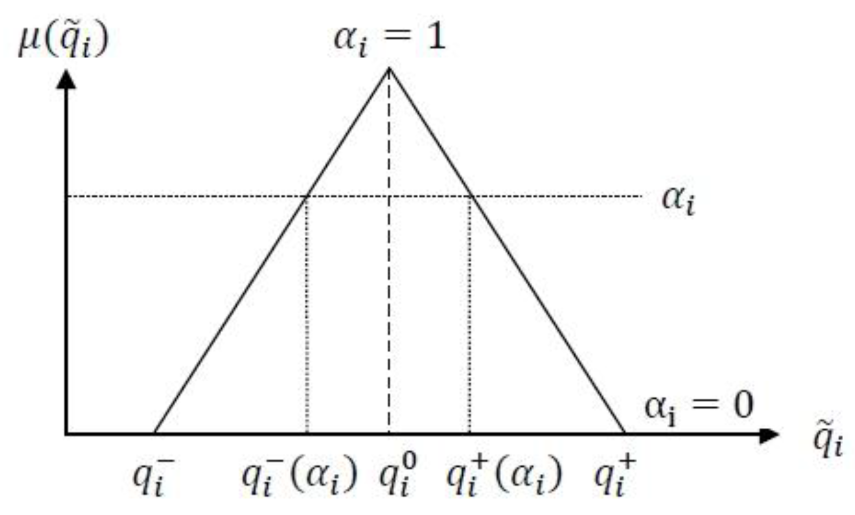
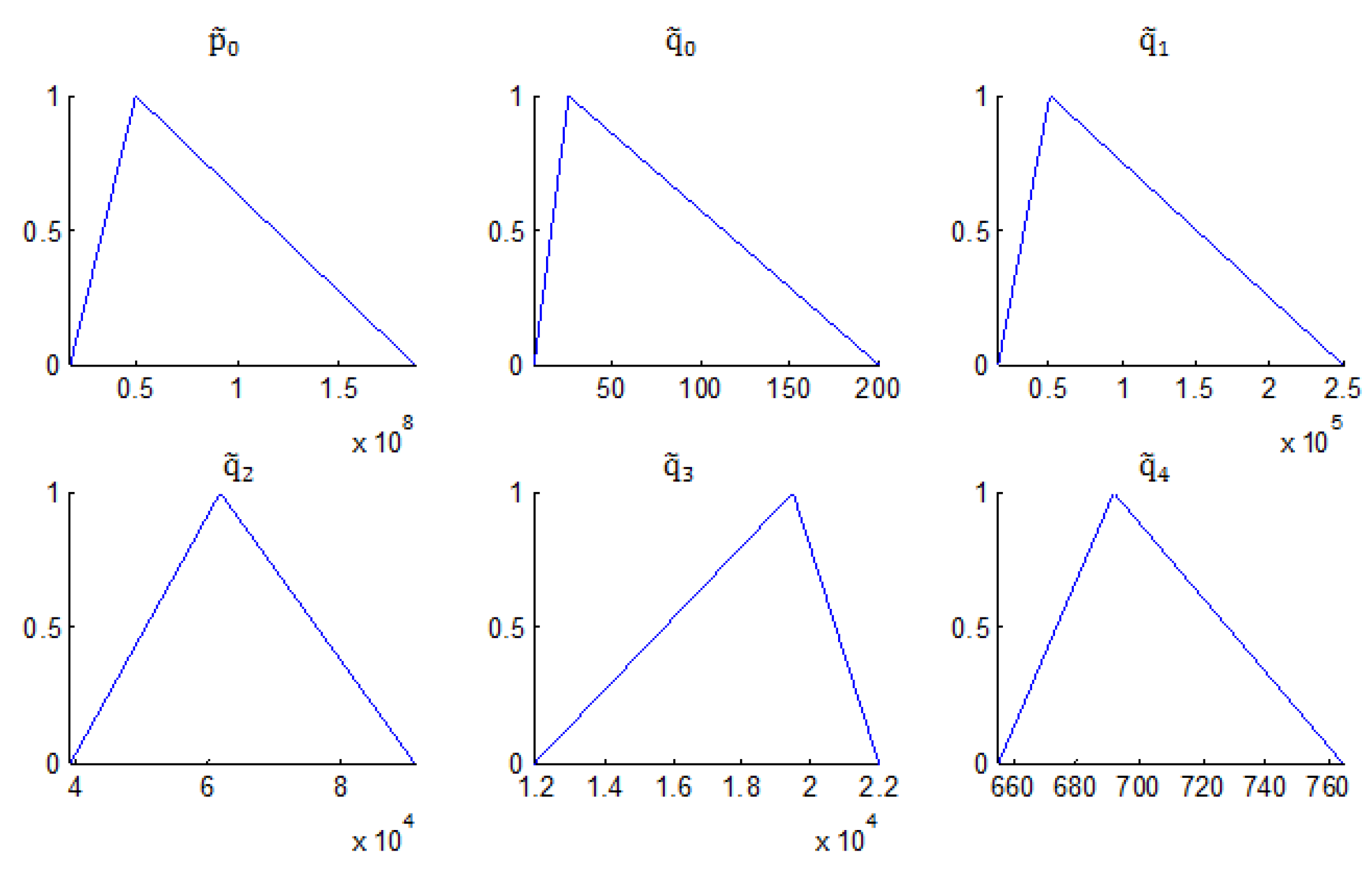
2.2. Fuzzy Parametric α-Cut Representation of the Uncertain HEV Model

The interval uncertainty representation assumes all of the parameters have the same probability. However, this is not true in practical applications. In this study, the uncertain parameters are represented by a fuzzy number q ˜ i with membership function α = μ ( q ˜ i ) [ 0 , 1 ] . The membership function μ ( q ˜ i ) can be any nonsymmetrical membership function, but decreases to the interval endpoint. The fuzzy parametric uncertainty α -cut is defined as:
q i ( α i ) = [ q i ( α i ) , q i + ( α i ) ]
where q i ( . ) is an increasing function and q i + ( . ) is a decreasing function. Let α i be the membership level of q i , as shown in Figure 2; we obtain:
q i ( 0 ) = q i ,   q i + ( 0 ) = q i + ,   q i ( 1 ) = q i + ( 1 ) = q i 0
Consider the uncertain interval model Equation (13). Assume that the only information available for the values of the uncertain parameters p ˜ 0 , q ˜ 0 , q ˜ 1 , q ˜ 2 , q ˜ 3 and q ˜ 4 , is the linguistic information “around the nominal value of Table 1”, by using interval arithmetic (affine linearization) [17,19,20]; the linguistic information can be represented as a fuzzy set with triangular membership functions, where p ˜ 0 = tri ( 1.7 × 10 7 , 5 × 10 7 , 1.87 × 10 8 ) , q ˜ 0 = tri ( 5.5 , 25.4 , 200 ) , q ˜ 1 = tri ( 1.56 × 10 4 , 5.08 × 10 4 , 2.5 × 10 5 ) , q ˜ 2 = tri ( 3.9 × 10 4 , 6.17 × 10 4 , 9.1 × 10 4 ) , q ˜ 3 = tri ( 1.19 × 10 4 , 1.95 × 10 4 , 2.2 × 10 4 ) and q ˜ 4 = tri ( 655 , 691.7 , 764 ) (Figure 3). For α -cut = 1, we obtain a nominal condition; for α -cut = 0, we obtain maximum uncertainty. The fuzzy numbers correspond to their own confidence level α -cut and can be interpreted as possibility distributions. Finally, the nonlinear HEV system can translate into a fuzzy parametric uncertain system with a degree of confidence of α [ 0 , 1 ] .
G N ( s , q i ( α = 1 ) ) = 5 × 10 7 s 5 + 691.7 s 4 + 1.95 × 10 4 s 3 + 6.17 × 10 4 s 2 + 5.08 × 10 4 s + 25.4 G L ( s , q i ( α = 0 ) ) = 1.87 × 10 8 s 5 + 764 s 4 + 1.19 × 10 4 s 3 + 9.1 × 10 4 s 2 + 2.5 × 10 5 s + 200 G U ( s , q i ( α = 0 ) ) = 1.7 × 10 7 s 5 + 655 s 4 + 2.2 × 10 4 s 3 + 3.9 × 10 4 s 2 + 1.56 × 10 4 s + 5.5
This paper focuses on the problem of longitudinal speed control for HEV systems. The designed controller must not only stabilize the fuzzy parametric uncertain system, but also satisfy the performance requirements.

3. Controller Design

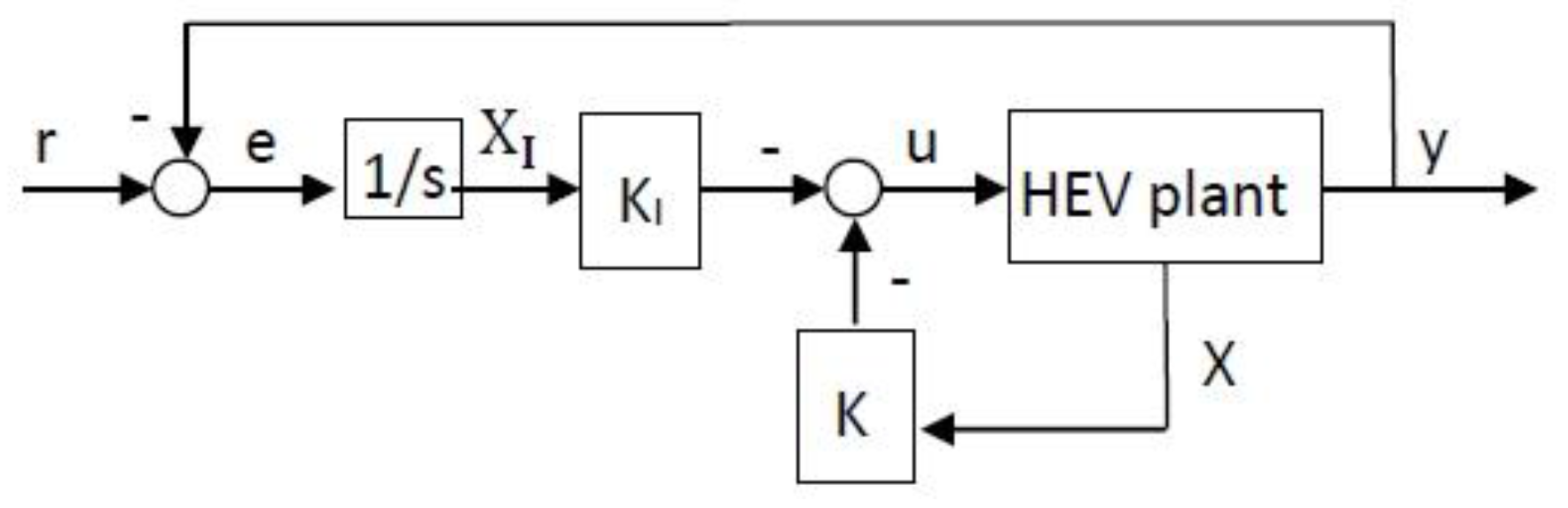
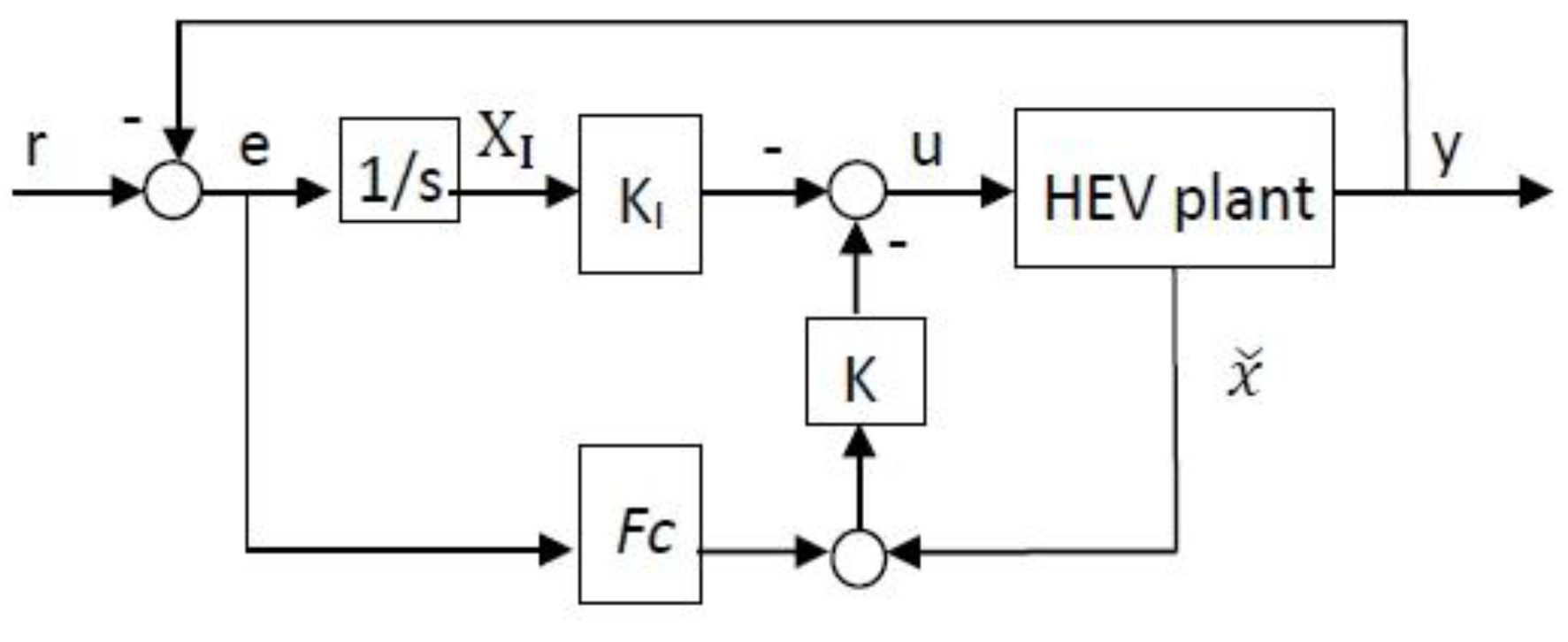
3.1. Optimal-Based Robust Feedback Controller Design

Nonlinear dynamic equations can be represented as linear models at specific operating points. When a nonlinear system can be stabilized at different operating points, it is equivalent to stabilizing the parametric uncertain linear model. Consider an uncertain system represented as a system with fuzzy parametric uncertainty, as described by the following transfer function:
G ( s , p ˜ ( α ) , q ˜ ( α ) ) = p ˜ n 1 ( α ) s n 1 + + p ˜ 1 ( α ) s + p ˜ 0 ( α ) s n + q ˜ n 1 ( α ) s n 1 + + q ˜ 1 ( α ) s + q ˜ 0 ( α )
where p ˜ i ( α ) , q ˜ i ( α ) represents the fuzzy interval number. The α -cut confidence is given as α [ 0 , 1 ] .
Furthermore, the fuzzy parametric uncertain system is realized in state-space representation by a controllable canonical form:
x ˙ = [ 0 1 0 0 0 1 q ˜ 0 ( α ) q ˜ 1 ( α ) q ˜ n 1 ( α ) ] x + [ 0 0 1 ] u y = [ p ˜ 0 ( α ) p ˜ 1 ( α ) p ˜ n 1 ( α ) ] x
The compact representation of Equation (18) is:
x ˙ = A ( q ˜ ( α ) ) x + B u y = C ( p ˜ ( α ) ) x
Assume that there exists a nominal value q n o m q ˜ ( α ) , such that ( A ( q n o m ) , B ) is stable; there exists a matrix ϕ ( q ˜ ( α ) ). The uncertainty in A is represented as:
A ( q ˜ ( α ) ) x A ( q n o m ) x = B ϕ ( q ˜ ( α ) )
The fuzzy parametric uncertain system can then be rewritten as:
x ˙ = A ( q n o m ) x + B ϕ ( q ˜ ( α ) ) + B u
The problem of designing a robust controller for a system with fuzzy parametric uncertainty lies in finding a feedback control law u = k x such that the closed loop system:
x ˙ = A ( q n o m ) x + B ϕ ( q ˜ ( α ) ) B k x
is stable for all α [ 0 , 1 ] . For the system with fuzzy parametric uncertainty in Equation (19), let the cost function be designed as:
J = 0 ( x T F x + x T x + u T R u ) d t
where F is an upper bound on the uncertainty. Now, the aforementioned robust control problem can be translated into an optimal control problem by using an LQR approach. Generally, the weighting matrices Q and R are often determined arbitrarily or based on trial and error. In this study, we assume the uncertain system ϕ ( q ˜ ( α ) ) is bounded; the upper bound on F can be written as:
ϕ ( q ˜ ( α ) ) T ϕ ( q ˜ ( α ) ) F
When Q = [ F + I ] , the cost function is rewritten as:
J = 0 ( x T Q x + u T R u ) d t
The LQR optimal control problem involves finding the optimal feedback gain u = k x that minimizes the cost function. When there exists a feedback control law u = k x , such that Equation (22) is stable for all q ˜ ( α ) , α [ 0 , 1 ] , the design of a robust controller is completed. For a system with fuzzy parametric uncertainty, the solution to the LQR problem is the solution to the robust control problem. The following proposition demonstrates how to determine the weighting matrix Q in the LQR problem.
For α = 0 , consider the maximum uncertainty described by q i [ q i ,   q i + ] . For α [ 0 , 1 ] , the uncertainty [ q i ( α i ) ,   q i + ( α i ) ] can be written as any value in [ q i ,   q i + ] . For the sake of demonstration, assume that the nominal value is q n o m = [ q 0 q 1 q n 1 ] . In Equation (21), the uncertain system B ϕ ( q ˜ ) can be written as:
[ 0 1 0 0 0 1 q ˜ 0 q ˜ 1 q ˜ n 1 ] [ 0 1 0 0 0 1 q 0 q 1 q n 1 ] = [ 0 0 1 ] [ q 0 q ˜ 0 q 1 q ˜ 1 q n 1 q ˜ n 1 ] T
The maximum uncertainty ϕ ( q ˜ ) is bounded by:
F = ϕ T ϕ = [ [ q 0 + q 0 ] [ q 0 + q 0 ] [ q 0 + q 0 ] [ q n 1 + q n 1 ] [ q n 1 + q n 1 ] [ q 0 + q 0 ] [ q n 1 + q n 1 ] [ q n 1 + q n 1 ] ]
Let Q = [ F + I ] , and designate Q as the cost function for the LQR optimal control problem. With the feedback control law u = k x , the characteristic equation of the closed loop system in Equation (22) can be written as:
s n + [ k n + q ˜ n 1 ] s n 1 + + [ k 2 + q ˜ 1 ] s + [ k 1 + q ˜ 0 ] = 0
Kharitonov’s theorem can be used to determine whether the interval polynomial is stable. If and only if all four Kharitonov extreme characteristic polynomials have roots in the left-half plane (LHP), the optimal feedback controller design is a solution to stabilize all of the systems for various values of α [ 0 , 1 ] .
For the linear quadratic tracking (LQT) problem, we cannot use the aforementioned algorithm directly. We must augment another system state. Define the augment system state x ˙ I ( t ) = e ( t ) = r ( t ) y ( t ) , and augment Equation (18) as:
[ x ˙ x ˙ I ] = [ A 0 C 0 ] [ x ( t ) x I ( t ) ] + [ B u 0 ] u ( t ) + [ 0 I ] r ( t ) X ¯ = [ x ˙ x ˙ I ]
Then, the cost function in Equation (25) will be rewritten as:
J = 0 ( X ¯ T Q X ¯ + u T R u ) d t
The tracking problem can be transformed into a stabilization problem. The block diagram for the HEV longitudinal speed control with a robust feedback controller is shown in Figure 4.

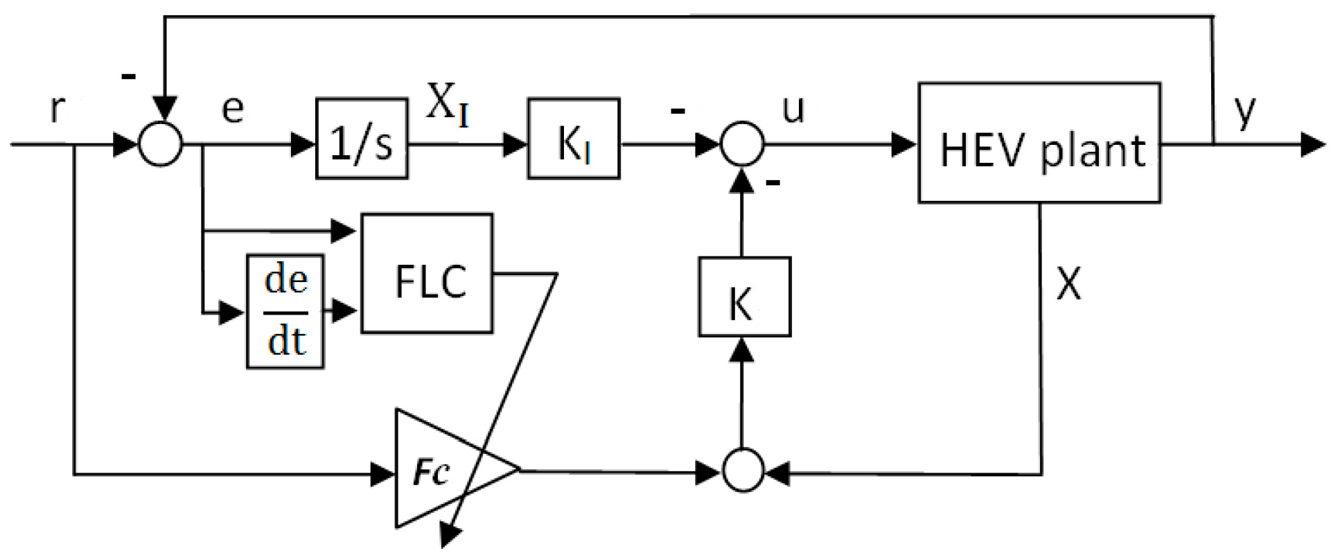
3.2. Fuzzy Logic Forward Compensator Design

For accurate speed tracking, we need a controller that can exhibit robustness in stability, as well as in tracking performance. In Section 3.1, we complete the design of the optimal linear quadratic (LQ) feedback controller with robustness. However, neglecting the nonlinearities of the system may result in an LQ controller with poor tracking performance. Combining the forward and feedback controllers can therefore satisfy the performance requirements.

3.2.1. Forward Compensator Fc Design

As shown in Figure 4, a concern about the architecture is that the response to the reference input is driven only by the integrated error. There is no forward path from the reference input to the system, and the transient response may be slow. This drawback can be mitigated by adding the forward compensator F C shown in Figure 5. The control law for the revised implementation can be written as:
u = K ( x ˇ + F c × e ) K I X I
Note that the tracking error includes the output of the integrator and the state feedback components. Thus, this type of 2-DoF approach has the potential to enhance the performance problems identified in the original implementation. The entire design process of the forward controller ( F C ) is described as follows.
Assume the state X of the HEV system in Figure 4 can be partitioned into x and x ˇ . x are the parts we care about for tracking ( T X ) that we assume are directly available from y = x = C X , and x ˇ are the parts we do not care about for tracking ( x ˇ = T ¯ X ). The matrices of T and T ¯ can be considered selectors with diagonals of one and zero, but they do not always take this form. Assume T ¯ is the complementary matrix of T ( T + T ¯ = I ) and state (vehicle speed) x is part of state vector X ( [ x , v , ] T ) ; let e = r C X , the control input u in Equation (31) is rewritten as:
u = K ( x ˇ F c × C X + F c × r ) K I X I
To proceed, define F C × C = T ; then:
x ˇ F c × C X = T ¯ X ( T ) X = X
Finally, the control input becomes:
u = K ( X + F c × r ) K I x I
Using T = F C × C ensures avoiding double counting in the feedback. Without loss of generality, we can use:
F c = γ C T ,   γ < 1
The entire closed-loop dynamics of the 2-DoF controller system is expressed as:
[ X ˙ X ˙ I ] = [ A B K B K I C 0 ] [ X X I ] + [ B K F c I ] r
Because of the nonlinear properties of HEV speed control, through Equations (16) and (35), the matrix C is not constant, but the fuzzy parametric uncertainty. To obtain optimal system performance, the weighting ( B K F C ) of forward compensator F C should not be constant, either. The next section discusses how to use fuzzy logic controllers (FLCs) to tune the B K F C of forward compensator F C .

3.2.2. The Weighting ( B K F c ) of Forward Compensator Tuning by FLC

An FLC is used to design the tuning of forward compensator F C . The inputs to the FLC are the error ( e = r y ) and change in error (ce), and the output variable is the B F C . The input triangular membership functions are designed according to five linguistic terms: positive big (PB), positive (P), zero (Z), negative (N) and negative big (NB). The output linguistic levels are assigned as small (S), medium small (MS), medium (M), medium big (MB) and big (B). Twenty-five rules for using the trial and error method are shown in Table 2. The entire system diagram is depicted in Figure 6.

3.3. Design Procedure

We summarize the design procedure for the proposed robust 2-DoF controller as follows.
  • Step 1: Linearize the nonlinear HEV model at specific operating points and represent as an uncertain interval model.
  • Step 2: The uncertain interval parameters are represented by a fuzzy number q ˜ with membership function α = μ ( q ˜ ) [ 0 , 1 ] . Translate the uncertain interval system into the fuzzy parametric uncertain system.
  • Step 3: For α = 0 , the maximum uncertain interval of the system is translated into the weighting matrix Q of the linear quadratic tracking (LQT) servo problem.
  • Step 4: Design an optimal controller for α = 0 , which can be considered as the worst case condition.
  • Step 5: Use Kharitonov’s theorem to test whether the optimal feedback controller is a solution to stabilize all of the systems for various values of α [ 0 , 1 ] .
  • Step 6: Design the FLC-based forward compensator to satisfy the performance requirements.

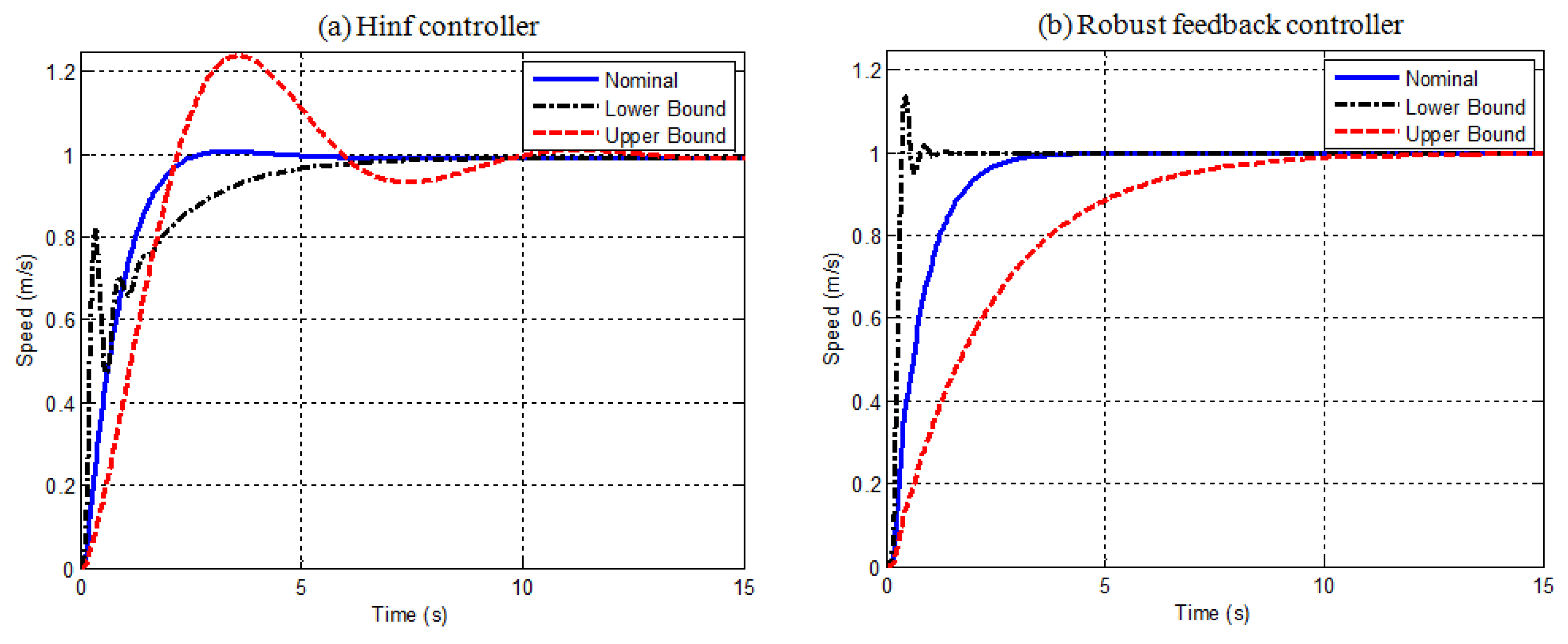
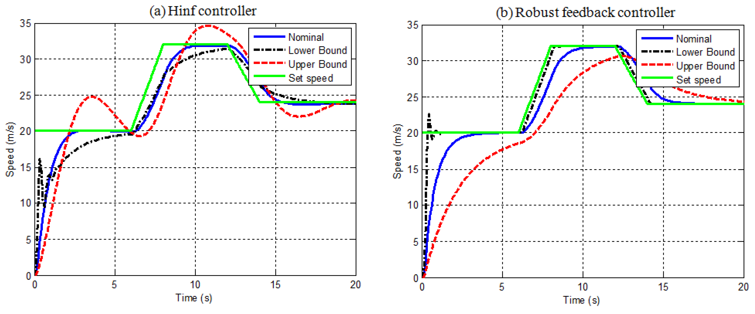
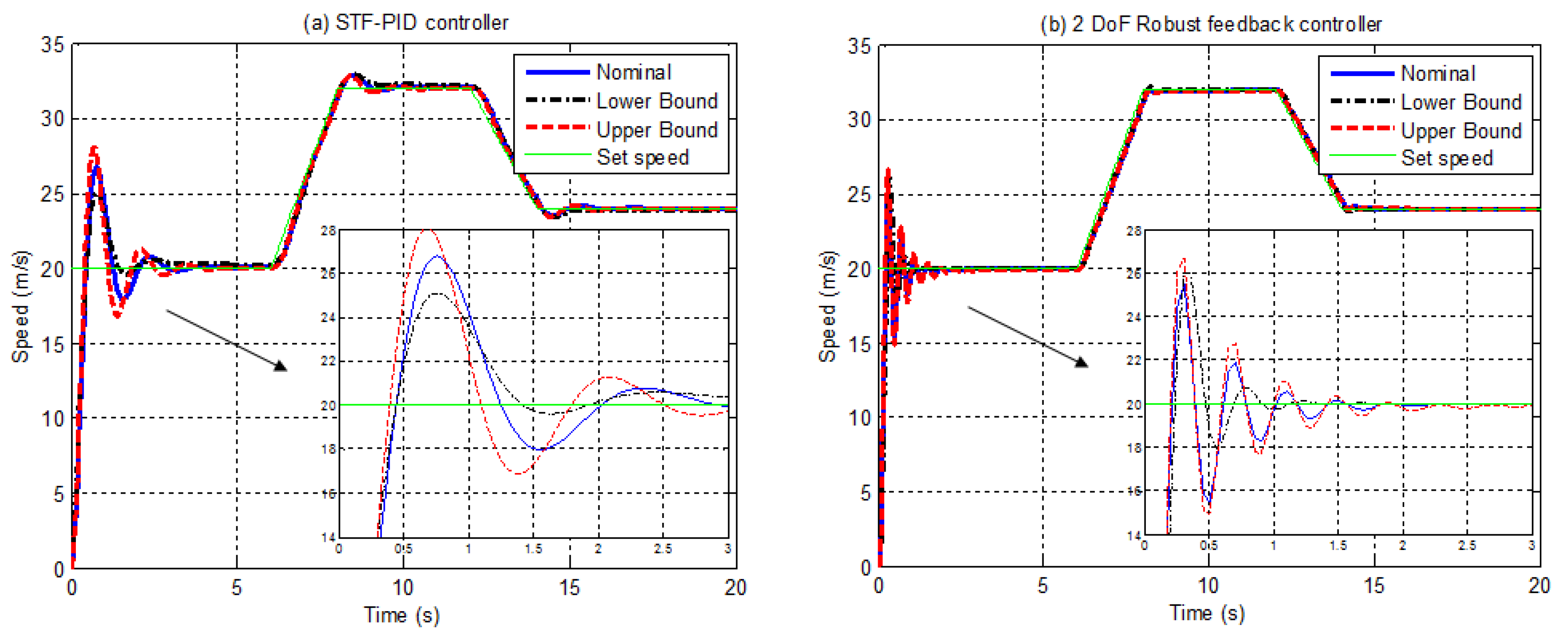
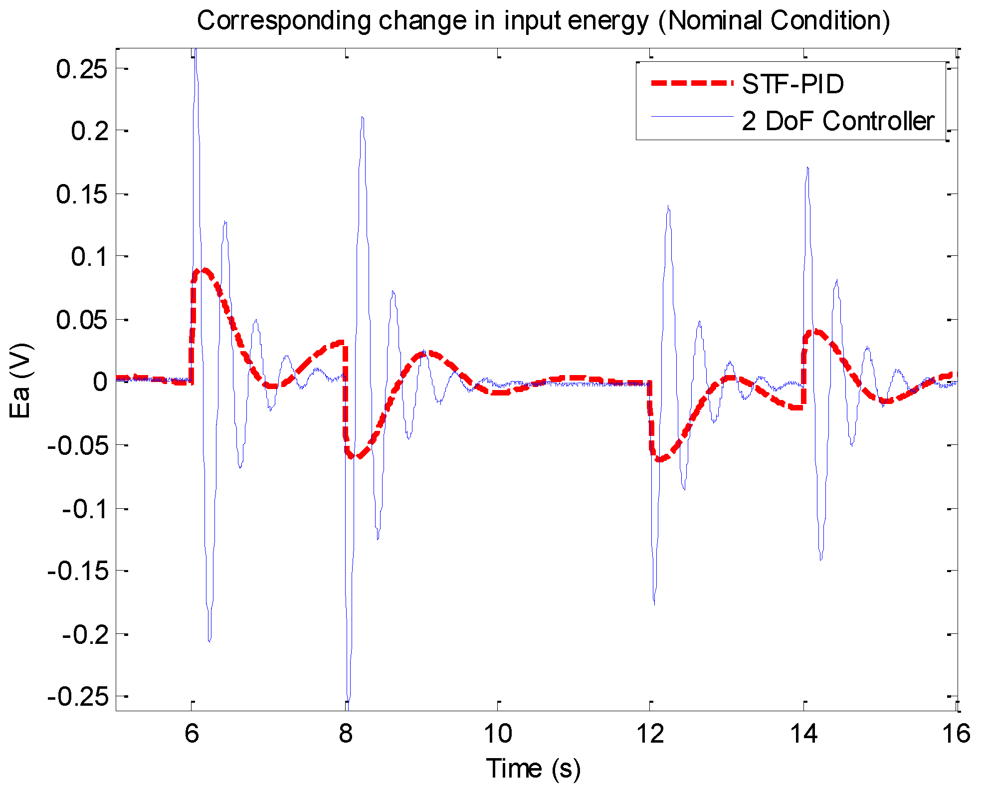
4. Simulation Results

This section illustrates how to design robust longitudinal speed control systems for HEVs based on a 2-DoF design method.

Simulation of Optimal Based Robust Feedback Controller

In Equation (16), the transfer function of the HEV system with parametric variation is expressed as:
G ˜ ( s ) = [ 1.87   17 ] × 10 8 s 5 + [ 655   764 ] s 4 + [ 1.19   2.2 ] × 10 4 s 3 + [ 3.9   9.1 ] × 10 4 s 2 + [ 1.56   25 ] × 10 4 s + [ 5.5   200 ]
For convenience, we translate this equation into its controllable canonical form, and the transfer function of the parametric uncertain system in Equation (21) is expressed as:
x ˙ [ 0 1 0 0 0 0 0 1 0 0 0 0 0 1 0 0 0 0 0 1 [ 5.5   200 ] [ 1.56   25 ] × 10 4 [ 3.9   9.1 ] × 10 4 [ 1.19   2.2 ] × 10 4 [ 655   764 ] ] A x + [ 0 0 0 0 1 ] B u u C = [ [ 1.87   17 ] × 10 8 0 0 0 0 ]
In order to satisfy the requirement of LQT, we augment the system Equations (38) to (29).
Using Equation (20), the maximum uncertainty ϕ ( q ˜ ) is bounded by:
ϕ ( q ˜ ) = [ 1.3 × 10 8 194.5 234 , 400 52 , 000 10 , 100 109 ]
The upper bound of the uncertainty in Equation (24) can be expressed as F = ϕ T ϕ . Then, the LQT weighting matrix Q can be written as [ F + I ] . Considering R = 1000 and solving the feedback control gain by using the LQT approach, we obtain K L Q T as follows:
K L Q T = [ 1.38 × 10 8 1.45 × 10 7 8.99 × 10 5 29096.8 98.5 3.45 ]
With the feedback control law, all four of Kharitonov’s extreme characteristic polynomials over all of the operating conditions can be expressed as:
k 1 ( s ) = s 6 + 753.5 s 5 + 40 , 997 s 4 + 9.9 × 10 5 s 3 + 1.47 × 10 7 s 2 + 1.38 × 10 8 s + 5.85 × 10 7 k 2 ( s ) = s 6 + 862.5 s 5 + 51 , 097 s 4 + 9.3 × 10 5 s 3 + 1.45 × 10 7 s 2 + 1.38 × 10 8 s + 6.45 × 10 8 k 3 ( s ) = s 6 + 862.5 s 5 + 40 , 997 s 4 + 9.3 × 10 5 s 3 + 1.47 × 10 7 s 2 + 1.38 × 10 8 s + 5.85 × 10 7 k 4 ( s ) = s 6 + 753.5 s 5 + 51 , 097 s 4 + 9.9 × 10 5 s 3 + 1.45 × 10 7 s 2 + 1.38 × 10 8 s + 6.45 × 10 8
We verify the conditions for robust stability in Equation (41) and find the entire fuzzy uncertain system to be stable. Furthermore, to demonstrate that the proposed feedback approach can consider robustness, we evaluate the proposed approach by comparing H methods [12] with different cruise-tracking regimes.
The step responses of the system with two kinds of feedback controller are shown in Figure 7. The comparison of the time domain performance indices in terms of the overshoot (OS), rise time (RT), delay time (DT) and settling time (ST) that correspond to transient state characteristics is shown in Table 3. Both control schemes stabilize the entire uncertain system. The simulation results show higher overshoot and longer settling times in the H controller. However, the proposed robust feedback controller yields longer response times.
Because the speed does not generally change stepwise in practical applications, trapezoidal speed profiles are used instead. In this case, the accurate tracking of the reference input during acceleration and deceleration is crucial. Again, the robust properties and tracking performance of the two control schemes are also assessed. The scenario of wide-range cruise-tracking performance is set as follows: the vehicle speed is 20 m/s for the first 6 s; there is then an acceleration at the rate of 6 m/s2; thence, the vehicle runs at a constant speed of 32 m/s for 8 to 12 s. For a time interval of 12 to 14 s, the vehicle runs in a decelerating mode at 4 m/s2, reaching 24 m/s; finally, from 14 to 20 s, the vehicle runs at a constant speed of 24 m/s. The wide-range cruise-tracking responses of the system with two types of feedback controllers are shown in Figure 8.
Although both the H feedback controller and proposed LQ feedback controller are robust because of high nonlinearities in the HEV system, when the range of operation is complex, the single-type feedback controller deteriorates in tracking performance. Figure 8 shows that the 1-DoF fixed-value controller cannot yield adequate tracking performance. To improve the slow transient response and enhance the tracking performance of the 1-DoF robust feedback controller, it can be paired with the forward compensator F C in Figure 6. The proposed 2-DoF fuzzy controller has an additional component to compensate for the effects of the response.
Based on Figure 6, the FLC is a two input and one output system. For successful implementation of the fuzzy forward compensator, we must estimate the maximum excursion of the input and output signals of the fuzzy controller. Using trial and error, the universe of discourse in fuzzy membership function designed for the error, the change of error and the output covers a range of [–10,20], [–25,25] and [0.25,7.5], respectively.
The tracking performance of the designed 2-DoF controller is analyzed by comparing it to that of the self-tuning fuzzy logic PID (STF-PID) controller in [12]. The integral error performance indices are used to obtain greater insight into HEV tracking performance with two controllers. The wide-range cruise-tracking responses of the system with two types of controllers are shown in Figure 9. The comparison of input energy for the period from t =5 s to t = 16 s in the nominal condition are shown in Figure 10. Table 4 shows the performance index analysis of the integral squared error (ISE) and integral absolute error (IAE).
The proposed 2-DoF controller uses more input energy to adjust the throttle position quickly to satisfy the performance requirement. Although the input energy of the proposed controller (0.0343) is bigger than that of STF-PID controller (0.0078), the performance of the proposed controller is higher than that of the STF-PID controller, as shown in Figure 9 and Table 4. Compared to the STF-PID controller, the maximum tracking errors (IAE, ISE) of the 2-DoF controller are smaller and reach 8.15 and 49.7, respectively. From the practical point of view, the accuracy of speed control is the key technology to improve many important applications of HEVs (E.g. adaptive cruise control, intelligent collision avoidance or car following). Besides, the accuracy of throttle position control can upgrade the fuel economy and reduce the pollutant emission. Furthermore, if the performance requirements concern the factor of input energy, based on the LQT character, the proposed methodology still has the flexibility to adjust the LQT weighting matrix R to reduce the magnitude of input energy.

5. Conclusions

In this paper, a 2-DoF robust fuzzy controller is successfully applied to the nonlinear uncertain HEV longitudinal speed control model. First, using the proposed algorithm, the uncertainty intervals of HEV dynamic systems are approximated by fuzzy α-cut coefficients. Subsequently, the maximum uncertainty interval is then translated into the weighting matrix Q of the LQT problem to guarantee that the designed optimal feedback controller is robust under various values of α [0,1]. The robust stability of the longitudinal speed control is analyzed using Kharitonov’s theorem. Finally, to compensate for the longer response time of the single-type feedback controller, the forward compensator is connected to enhance tracking performance. In contrast to many previously-proposed nonlinear controllers, our controller is easy to understand and implement. The proposed 2-DoF method was successfully applied in speed tracking control of HEVs and can also be extended to general servo control design.

Acknowledgments

This paper was supported by the Ministry of Science and Technology, Taiwan (No. MOST 104-3011-E-110-001).

Author Contributions

Yi-Horng Lai wrote this manuscript and contacted the editor. Jau-Woei Perng was in charge of the research architecture and revising the English editing in this manuscript.

Conflicts of Interest

The authors declare no conflict of interest.

References

  1. Liu, T.; Zou, Y.; Liu, D.; Sun, F. Reinforcement Learning-Based Energy Management Strategy for a Hybrid Electric Tracked Vehicle. Energies 2015, 8, 7243–7260. [Google Scholar] [CrossRef]
  2. Fu, Z.; Gao, A.; Wang, X.; Song, X. Torque Split Strategy for Parallel Hybrid Electric Vehicles with an Integrated Starter Generator. Discret. Dyn. Nat. Soc. 2014, 2014. [Google Scholar] [CrossRef]
  3. He, H.; Sun, C.; Zhang, X. A Method for Identification of Driving Patterns in Hybrid Electric Vehicles Based on a LVQ Neural Network. Energies 2012, 5, 3363–3380. [Google Scholar]
  4. Moura, S.J.; Fathy, H.K.; Callaway, D.S.; Stein, J.L. A Stochastic Optimal Control Approach for Power Management in Plug-in Hybrid Electric Vehicles. IEEE Trans. Control Syst. Technol. 2011, 19, 545–555. [Google Scholar] [CrossRef]
  5. Assadian, F.; Fekri, S.; Hancock, M. Hybrid electric vehicles challenges: Strategies for advanced engine speed control. In Proceedings of the 2012 IEEE International Conference in Electric Vehicle (IEVC), Greenville, SC, USA, 4–8 March 2012; pp. 1–8.
  6. Yan, C.; Junmin, W. Adaptive Vehicle Speed Control With Input Injections for Longitudinal Motion Independent Road Frictional Condition Estimation. IEEE Trans. Veh. Technol. 2011, 60, 839–848. [Google Scholar]
  7. Vajedi, M.; Azad, N.L. Ecological Adaptive Cruise Controller for Plug-In Hybrid Electric Vehicles Using Nonlinear Model Predictive Control. IEEE Trans. Intell. Transp. Syst. 2015, 17, 113–122. [Google Scholar] [CrossRef]
  8. Yu, K.; Mukai, M.; Kawabe, T. Performance of an Eco-Driving Model Predictive Control System for HEVs during Car Following. Asian J. Control 2015, 7, 55–62. [Google Scholar] [CrossRef]
  9. Conatser, R.; Wagner, J.; Ganta, S.; Walker, I. Diagnosis of automotive electronic throttle control systems. Control Eng. Pract. 2004, 12, 23–30. [Google Scholar]
  10. Zulkifli, S.A.; Asirvadam, V.S.; Saad, N.; Aziz, A.R.A.; Mohideen, A.A.M. Implementation of electronic throttle-by-wire for a hybrid electric vehicle using National Instruments’ CompactRIO and LabVIEW Real-Time. In Proceedings of the 2014 5th International Conference in Intelligent and Advanced Systems (ICIAS), Kuala Lumpur, Malaysia, 3–5 June 2014; pp. 1–6.
  11. Shupeng, Z.; Yang, J.J.; Zhu, G.G. LPV Modeling and Mixed Constrained H2/Hinf Control of an Electronic Throttle. IEEE/ASME Trans. Mechatron. 2015, 20, 2120–2132. [Google Scholar]
  12. Yadav, A.; Gaur, P. Robust adaptive speed control of uncertain hybrid electric vehicle using electronic throttle control with varying road grade. Nonlinear Dyn. 2014, 76, 305–321. [Google Scholar]
  13. Li, Y.; Yang, B.; Zheng, T.; Li, Y. Extended State Observer Based Adaptive Back-Stepping Sliding Mode Control of Electronic Throttle in Transportation Cyber-Physical Systems. Math. Probl. Eng. 2015, 2015, 1–11. [Google Scholar]
  14. Yadav, A.K.; Gaur, P. Intelligent modified internal model control for speed control of nonlinear uncertain heavy duty vehicles. ISA Trans. 2015, 56, 288–298. [Google Scholar] [CrossRef] [PubMed]
  15. Chamsai, T.; Jirawattana, P.; Radpukdee, T. Robust Adaptive PID Controller for a Class of Uncertain Nonlinear Systems: An Application for Speed Tracking Control of an SI Engine. Math. Probl. Eng. 2015, 2015, 12. [Google Scholar] [CrossRef]
  16. Yadav, A.K.; Gaur, P.; Jha, S.K.; Gupta, J.R.P.; Mittal, A.P. Optimal Speed Control of Hybrid Electric Vehicles. J. Power Electron. 2011, 11, 393–400. [Google Scholar] [CrossRef]
  17. Bhiwani, R.J.; Patre, B.M. Stability analysis of fuzzy parametric uncertain systems. ISA Trans. 2011, 50, 538–547. [Google Scholar] [CrossRef] [PubMed]
  18. Tao, C.W.; Taur, J.S. Robust fuzzy control for a plant with fuzzy linear model. IEEE Trans. Fuzzy Syst. 2005, 13, 30–41. [Google Scholar] [CrossRef]
  19. Bhiwani, R.J.; Patre, B.M. Design of Robust PI/PID Controller for Fuzzy Parametric Uncertain Systems. Int. J. Fuzzy Syst. 2011, 13, 16–23. [Google Scholar]
  20. Patre, B.M.; Bhiwani, R.J. Robust controller design for fuzzy parametric uncertain systems: An optimal control approach. ISA Trans. 2013, 52, 184–191. [Google Scholar] [CrossRef] [PubMed]
  21. Barai, R.K.; Nonami, K. Optimal two-degree-of-freedom fuzzy control for locomotion control of a hydraulically actuated hexapod robot. Inf. Sci. 2007, 177, 1892–1915. [Google Scholar] [CrossRef]
  22. Harnefors, L.; Saarakkala, S.E.; Hinkkanen, M. Speed Control of Electrical Drives Using Classical Control Methods. IEEE Trans. Ind. Appl. 2013, 49, 889–898. [Google Scholar] [CrossRef]
  23. Nam, K.; Oh, S.; Fujimoto, H.; Hori, Y. Robust yaw stability control for electric vehicles based on active front steering control through a steer-by-wire system. Int. J. Automot. Technol. 2012, 13, 1169–1176. [Google Scholar] [CrossRef]
Figure 1. The speed control scheme of the HEV with an electronic throttle control system (ETCS) and a nonlinear vehicle dynamic system.
Energies 09 00290 g001
Figure 2. Fuzzy α -cut representation of the uncertain parameter.
Energies 09 00290 g002
Figure 3. Membership function for p ˜ 0 , q ˜ 0 , q ˜ 1 , q ˜ 2 , q ˜ 3 and q ˜ 4 .
Energies 09 00290 g003
Figure 4. Block diagram for the HEV longitudinal speed control with robust feedback controller.
Energies 09 00290 g004
Figure 5. Block diagram for the HEV longitudinal speed control with forward compensator.
Energies 09 00290 g005
Figure 6. Block diagram for the HEV longitudinal speed control with the 2-DoF fuzzy controller. FLC, fuzzy logic controller.
Energies 09 00290 g006
Figure 7. Step response for the HEV speed control (a) with the H controller and (b) with the robust feedback controller.
Energies 09 00290 g007
Figure 8. Wide range cruise tracking response for the HEV speed control (a) with the H controller and (b) with the robust feedback controller.
Energies 09 00290 g008
Figure 9. Wide range operation response for the HEV speed control (a) with STF-PID and (b) with the 2-DoF robust controller.
Energies 09 00290 g009
Figure 10. Corresponding change in input energy for the period from t = 5 s to t = 16 s.
Energies 09 00290 g010
Table 1. The nominal values and uncertainty parameters of the HEV.
ETCS
DescriptionsSymbolNominal Value (SI unit)Uncertainty Bounds
Armature resistance R a 2 Ω [1.5,2.5]
Armature inductance L a 0.003 H[0.002,0.004]
Back electromotive force (EMF) constant K b 0.11 Vs/rad[0.07,0.15]
Gear ratio N 4[2,6]
Motor torque constant K t 0.1 N m/A[0.08,0.12]
Throttle spring constant K s p 0.4 N ms/rad[0.3,0.5]
Equivalent inertia J 0.021 kg m 2 [0.009,0.0502]
Damping constant B 0.482 N ms/rad[0.082,1.443]
Vehicle Dynamic Model
DescriptionsSymbolNominal Value (SI unit)Uncertainty Bounds
Vehicle mass m 1000 kg[750,1250]
Drag coefficient α 0.48 N/ ( m / s ) 2 [0.4,0.56]
Engine force coefficient γ 12500 N[10000,15000]
Engine idle force F i 6400 N[5500,7300]
Engine time constancy τ e 0.5 s[0.2,0.8]
Bearing damping coefficient b w 0.035 N ms/rad[0.03,0.04]
Radius of tire r t i r e 70 mm[50,90]
Friction coefficient μ 0.011[0.01,0.012]
Road slope/grade β Variable[ ± 2 ° , ± 30 ° ]
Table 2. The rule base of the FLC: positive big (PB), positive (P), zero (Z), negative (N), negative big (NB), small (S), medium small (MS), medium (M), medium big (MB) and big (B).
ErrorNBNZPPB
Change in Error
NBSSMSMSM
NSMSMSMMB
ZMSMSMMBMB
PMSMMBMBB
PBMMBMBBB
Table 3. The comparison of the time domain performance index: overshoot (OS), rise time (RT), delay time (DT) and settling time (ST).
ControllerConditionOS (%)RT (s)DT (s)ST (s)
H controllerNominal1.3691.590.632.17
Lower Bound02.860.25.27
Upper Bound25.131.921.138.99
Proposed feedback controllerNominal01.70.612.8
Lower Bound13.370.310.240.72
Upper Bound05.271.678.77
Table 4. The comparison of the integral error performance index. IAE, integral absolute error; ISE, integral squared error; STF, self-tuning fuzzy logic.
IAEISE
ControllerNominalLowerUpperNominalLowerUpper
STF-PID13.5812.9413.2786.8068.7788.18
2-DoF controller7.356.598.1544.5949.0745.84

