Crop Management Effects on the Energy and Carbon Balances of Maize Stover-Based Ethanol Production

Abstract

This study was conducted to identify the crop management options—the combinations of various cultivars, irrigation amounts, planting dates, and soils—that would maximize the energy sustainability and eco-friendliness of maize (Zea mays L.) stover-based ethanol production systems in the Mississippi Delta. Stover yields simulated with CERES-Maize were used to compute net energy value (NEV) and carbon credit balance (CCB), the indicators of sustainability and eco-friendliness of ethanol production, respectively, for various scenarios. As the results showed, deeper soils with higher water holding capacities had larger NEV and CCB values. Both NEV and CCB had sigmoid relationships with irrigation amount and planting date and could be maximized by planting the crop during the optimum planting window. Stover yield had positive effects on NEV and CCB, whereas travel distance had negative. The influence of stover yield was larger than that of travel distance, indicating that increasing feedstock yields should be emphasized over reducing travel distance. The NEV and CCB values indicated that stover-based ethanol production in the Mississippi Delta is sustainable and environmentally friendly. The study demonstrated that the energy sustainability and eco-friendliness of maize stover-based ethanol production could be increased with alternative crop management options.

1. Introduction

Ethanol is being promoted as an alternative energy source due to its economic, environmental, societal, and strategic benefits [1,2,3,4,5,6,7]. Ethanol can be produced from plant materials such as lignocellulose, starch, and sugar. Ethanol production from starch and sugar, however, has issues related to environment, food security, and grain price increase [8,9]. Lignocellulosic ethanol, on the other hand, can displace more non-renewable energy and reduce environmental risks more efficiently than can starch- or sugar-based ethanol [10,11]. Also, lignocellulosic feedstocks are abundant, relatively cheap, and widely available [7,12,13,14]. The United States has an annual potential of producing about 189 million m³ of biofuels from lignocellulosic feedstocks [12]. Lignocellulosic ethanol production technology is still evolving, and once streamlined, lignocellulosic biomass has the potential to make substantial contribution toward biofuel production [15]. One of the most suitable and abundantly available lignocellulosic feedstocks is maize (Zea mays L.) stover, the above-ground portion of the maize plant minus the grains [16,17]. In the USA, maize is a principal feedstock for ethanol production [18] and is expected to contribute approximately 42% of the target annual use of biofuels in the country by 2022 [19].

Maize biomass yield is influenced by a number of environmental and management factors. Variation in cultivar, irrigation amount, planting date, or soil type can cause a considerable variation in maize stover yield. Accordingly, alterations in these variables might also affect non-renewable energy displacement and carbon emissions associated with maize stover-based ethanol production [20,21]. Previous studies that examined these issues did not specifically address the effects of cultivar, irrigation, planting date, and soil type on maize stover yield and stover-based ethanol production systems [20,21,22].

Biofuel production is associated with the issue of non-renewable energy displacement or energy sustainability [2,3,5,6]. The sustainability of biofuel production can be quantified using net energy value (NEV), a measure defined as the difference between renewable energy produced and non-renewable energy used to produce the renewable energy [23]. While a positive NEV value is an indication of a sustainable system, a larger NEV value indicates that the system is more sustainable.

Another important issue regarding biofuel production is CO₂ emissions during feedstock delivery and ethanol processing [24,25]. The increasing level of CO₂ in the atmosphere has been identified as a cause of global warming [2,26], a driver of several environmental problems. With the rise in concern about global climate change, therefore, studying CO₂ emissions becomes more and more important. For determining the effect of biofuel production on the environment, many previous studies have used CO₂ emissions as a basis. With a rise in stover yield, CO₂ emissions increase due to more material to harvest, transport, and process. During these activities, about 95.72 kg CO₂ is emitted for each Mg of stover [24,25]. The yield increase is beneficial; the associated emissions increase, however, is not. To reflect the positive aspect of yield increase as well as the negative aspect of a rise in emissions, a system of measurement called the carbon credits balance (CCB; [20]) can be used. One carbon credit can be regarded as a reward for extracting one Mg of CO₂ gas from the atmosphere. The CCB is defined as the amount of CO₂ (Mg) taken up by a maize plant from the atmosphere through fixation and stored in the stover minus the amount of CO₂ (Mg) emitted to the atmosphere through burning of fossil fuel for supplying a given quantity of stover to a biorefinery and processing it. Supply includes all activities in the feedstock supply chain, namely harvesting, collection, storage, and transportation. While a positive CCB value is indicative of an environmentally friendly ethanol production system (in terms of carbon emissions reduction), a larger value is an indication of a more environmentally friendly system.

Among the various regions of the USA, the southeastern region is more suitable for biomass production due to long crop growing seasons and high rainfall [27]. Due to an increase in the demand for ethanol, an interest in cultivating maize for ethanol production is growing in this country. In Mississippi, a southeastern state, favorable environmental conditions make biomass production a potential source of income for farmers. The large historical in addition to recently increasing maize area, as well as increasing maize yields, increasing switch of farmers from cotton to maize, and favorable climate and soil conditions for maize production in Mississippi all suggest that a large area is potentially available for maize stover-based ethanol production in this state [28,29]. The climate, soils, and other crop-growing conditions in Mississippi are also representative for other states in the southeastern USA. Although the southeastern region has good potential for lignocellulosic ethanol production, the production is still limited to the experimental scale [30]. The response of ethanol production systems to various environmental and crop management factors are largely unknown for this region [22,31,32]. Detailed knowledge about the impacts of variability in management and environment on the sustainability and eco-friendliness of maize stover-based ethanol production systems might be helpful in evaluating maize stover as a potential energy feedstock. Thus, additional information is needed to characterize the sustainability and eco-friendliness of maize stover-based ethanol production systems as influenced by management and environmental factors such as cultivar, irrigation, planting date, and soil.

The objective of this study was to identify the crop management options—the combinations of various management variables, namely cultivar, irrigation, planting date, and soil—that would maximize the energy sustainability and eco-friendliness of maize stover-based ethanol production systems in the Mississippi Delta. Specifically, this study examined how variations in these management variables would affect the NEV and CCB of maize stover-based ethanol production systems using crop modeling approach.

2. Materials and Methods

2.1. Sites and Data

For the study, the Mississippi Delta—an alluvial plain in northwestern Mississippi—was selected. The largest agricultural area in the state of Mississippi [33], the Delta region, has land use greater than 90% as agriculture and contributes significantly to the state’s economy. Maize is a primary crop in the region. Taking into account maize growing area, weather data availability, and geographical distribution, three locations in the Mississippi Delta were chosen for the study: Moorhead (center), Tunica (far north), and Vicksburg (far south).

For each location, daily weather data of minimum and maximum temperatures and precipitation for the climatic normal period of 1971–2000 were obtained from the Delta Agricultural Weather Center (http://www.deltaweather.msstate.edu) and the National Climate Data Center (http://www.ncdc.noaa.gov/oa/climate/stationlocator.html). Daily values of solar radiation for these locations and years were estimated using the WP model (Equation (16) of Woli and Paz [34]). Figure 1 shows the 30-year-average daily values of mean temperature and solar radiation at these locations during maize growing seasons.

Figure 1. The 30-year-average (1971–2000) daily values of: (a) Mean temperature; (b) Solar radiation at three locations in the Mississippi Delta during maize growing season.

Figure 1. The 30-year-average (1971–2000) daily values of: (a) Mean temperature; (b) Solar radiation at three locations in the Mississippi Delta during maize growing season.

2.2. Experimental Design

This study examined the effects of four factors on NEV and CCB: cultivar, irrigation, planting date, and soil type. Based on the suitability to growing maize and the proportion of availability in the region, the three most dominant soils were considered: sandy loam, silt loam, and silt clay loam [35].

No cultivar, including the ones used in the variety performance trials of the Mississippi State University Extension Service (MSUES; http://msucares.com/pubs/crops3.html#grain), the most reliable source of these data, was found to have been grown for a number of locations and years in the region. In order to establish consistency, recognizing the fact that new cultivars are established every year, the average of the top five highest grain yields of the Mississippi State University Extension Service performance trials each year was assumed to be the yield of AvTop5, a hypothetical cultivar. Additionally, three more cultivars were considered. The performance trial data contained many cultivars of several seed companies. From the list of companies, the Dyna-Gro Seed (http://www.dynagroseed.com) was chosen as it is one of the most popular companies for seeds in the region. From the yield records of Dyna-Gro every year, highest, average, and lowest values were taken and considered as the yields of hypothetical cultivars DynaGro-High, DynaGro-Mid, and DynaGro-Low, respectively.

For irrigation, five treatments were considered. In crop model simulations, irrigation was automatically applied based on the threshold, known as the management allowed depletion, the fraction of total plant-available water capacity that is to be depleted from the active root zone before irrigation is applied. When soil water content in the management depth, 40 cm [32], would fall below the threshold of a certain percent, irrigation in simulations would automatically be given to bring the soil water content back to the capacity. In this study, five threshold values (treatments) were considered: 0, 25, 50, 75, and 90. In the threshold 0, irrigation would be applied only when the plant-available water in the management depth would completely deplete. In the thresholds 25, 50, 75, and 90, irrigation would not be applied until the plant-available water would deplete down to 25%, 50%, 75%, and 90% of the available water capacity, respectively. For simplicity, the thresholds 0, 25, 50, 75, and 90 hereinafter are referred to as no, light, moderate, heavy, and extreme irrigations, respectively. The irrigation effects were studied for three weather conditions: dry, wet, and average. For dry (wet) condition, the driest (wettest) year was chosen for each location from the 1971–2000 period. For an average condition, all 30 years were considered. The driest and wettest years were determined based on the amount of precipitation within the crop-growing season.

In the Mississippi Delta, maize is generally planted from the beginning of March to the end of April [36]. Considering the fact that maize in southeastern USA can be planted from early March through early July [37], the planting window for the Delta region was considered to be early March through late May. Thus, 12 planting dates were created at one-week intervals: 4 March, 11 March, and so on, until 25 May.

2.3. Model Calibration

This is a simulation study. Maize yields, which later were used to compute NEV and CCB, were simulated using Crop Environment Resource Synthesis (CERES)-Maize [38], a widely tested and used model [39,40,41,42,43,44] coupled to the Decision Support System for Agrotechnology Transfer (DSSAT Version 4.0) [45,46], a suite of computer programs that facilitate the application of crop models. The CERES-Maize model needs to be calibrated, that is, its six cultivar coefficients need to be estimated for every cultivar that does not have coefficients previously estimated for the region. The six cultivar coefficients are: P1, the thermal time from seedling emergence to the end of juvenile phase (°C·days); P2, extent to which development is delayed for each hour increase in the photoperiod above the longest photoperiod at which development occurs at a maximum rate (days); P5, the thermal time from silking to physiological maturity (°C·days); G2, maximum possible kernels per plant (number); G3, kernel filling rate (mg·day⁻¹); and PHINT, phylochron interval between successive leaf tip appearances (°C·days). Considering that cultivars adapted to southeastern USA have low photoperiod sensitivity, 0.2 was assumed for P2 due to the unavailability of anthesis date data to calibrate with [47]. Similarly, due to the lack of information, PHINT was assumed to be 45 based on experience. Using the P2 and PHINT values, P1 was estimated through simulating a leaf number of 18 for the short-season cultivars. Values of P5, G2, and G3 were estimated following the procedures of Boote [48].

For estimating the cultivar coefficients for each cultivar, 17 observed yields of maize along with their planting and physiological maturity dates were used. The number of observed values was limited by the availability of historical weather data and the MSUES trials. Most properties of soils on which the trials had been conducted were obtained from the Soil Data Access (http://sdmdataaccess.nrcs.usda.gov/). The values of drained upper limit and lower limit, saturated water content, drainage coefficient, and runoff curve number were estimated using the techniques of Rawls et al. [49], Dalgliesh and Foale [50], Suleiman and Ritchie [51], and the United States Department of Agriculture (USDA) Natural Resources Conservation Service [52], respectively. The daily weather data related to the observed yields were obtained from the Delta Agricultural Weather Center (http://www.deltaweather.msstate.edu).

After the cultivar coefficients were estimated, the performance of the CERES-Maize model was evaluated using leave-one-out cross validation as the technique and root mean square error (RMSE), percent error (PE), coefficient of determination (R²), and the Willmott index (d-index; [53]) as the measures of fit. The d-index, represented as the ratio of mean squared error to the potential error, is a measure of the degree to which the observed values are approached by the model-predicted values. Its values range from 0 to 1, with 0 indicating no agreement between the observed and predicted values and 1 indicating the perfect agreement. The d-index overcomes the insensitivity of R² to differences in the observed and predicted means and variances [54] and is also better than PE as the general utility of PE is questionable because it is unbounded and unstable when the mean observed value or the number of observation becomes small. A good model’s d-index should approach 1 and the RMSE or PE 0. For a good model, PE ≤ 10 and d-index > 0.94, and for an acceptable or satisfactory model, R² > 0.5, 10 ≤ PE ≤ 20, and d-index > 0.86 [55,56].

2.4. Yield Simulation

For each location and each of the 30 maize growing seasons of 1971 through 2000, maize grain yields were simulated for 720 scenarios (3 soils × 4 cultivars × 5 irrigations × 12 planting dates). Soils were assumed to be in standard fertility conditions, so no fertilizer balance was simulated. Seed rate and row spacing were specified as 7.9 kg·m⁻² and 75 cm, respectively [57]. The soil profile data used in simulations were obtained following the procedure explained in Section 2.3 (Table 1).

Table 1. Various properties of three soil types at three locations in the Mississippi Delta.

Location Soil b		Property a
		Depth (cm)	Sand (%)	Silt (%)	Clay (%)	LL (v/v)	DUL (v/v)	WHC (v/v)	SOC (%)	CEC (mmol/g)
Tunica	SA	203	61.0	25.1	13.9	0.10	0.20	0.10	0.49	0.10
	SL	152	18.1	59.0	22.8	0.10	0.33	0.23	0.30	0.09
	SC	152	18.3	45.6	36.1	0.20	0.36	0.16	0.60	0.22
Moorhead	SA	152	53.2	24.4	22.5	0.08	0.21	0.13	0.37	0.09
	SL	152	11.1	66.7	22.2	0.13	0.34	0.21	0.42	0.19
	SC	152	20.9	50.7	28.4	0.15	0.32	0.17	0.42	0.17
Vicksburg	SA	203	52.6	20.5	26.9	0.05	0.28	0.23	0.63	0.22
	SL	152	14.5	73.3	12.2	0.08	0.27	0.19	0.37	0.07
	SC	203	7.1	66.4	26.5	0.16	0.35	0.19	0.43	0.19

Notes: ^a LL = soil water content at lower limit (wilting point); DUL = water content at drained upper limit (field capacity); WHC = water holding capacity, SOC = soil organic carbon; CEC = cation exchange capacity. ^b SA = sandy loam; SL = silt loam; SC = silty clay loam.

Table 1. Various properties of three soil types at three locations in the Mississippi Delta.

Location Soil b		Property a
		Depth (cm)	Sand (%)	Silt (%)	Clay (%)	LL (v/v)	DUL (v/v)	WHC (v/v)	SOC (%)	CEC (mmol/g)
Tunica	SA	203	61.0	25.1	13.9	0.10	0.20	0.10	0.49	0.10
	SL	152	18.1	59.0	22.8	0.10	0.33	0.23	0.30	0.09
	SC	152	18.3	45.6	36.1	0.20	0.36	0.16	0.60	0.22
Moorhead	SA	152	53.2	24.4	22.5	0.08	0.21	0.13	0.37	0.09
	SL	152	11.1	66.7	22.2	0.13	0.34	0.21	0.42	0.19
	SC	152	20.9	50.7	28.4	0.15	0.32	0.17	0.42	0.17
Vicksburg	SA	203	52.6	20.5	26.9	0.05	0.28	0.23	0.63	0.22
	SL	152	14.5	73.3	12.2	0.08	0.27	0.19	0.37	0.07
	SC	203	7.1	66.4	26.5	0.16	0.35	0.19	0.43	0.19

Notes: ^a LL = soil water content at lower limit (wilting point); DUL = water content at drained upper limit (field capacity); WHC = water holding capacity, SOC = soil organic carbon; CEC = cation exchange capacity. ^b SA = sandy loam; SL = silt loam; SC = silty clay loam.

Maize stover yields were estimated from the simulated maize grain yields, assuming the grain to stover ratio of 1:1 [58,59,60,61]. Because CERES-Maize has not been tested and widely used for stover yield simulation purpose, the simulated stover (non-grain component) yields were not used. An alternative and probably a better approach could be to parameterize the model to simulate the stover, evaluate the model for stover production systems, and then apply the model to estimate stover. Due to the lack of data, however, this approach could not be applied.

2.5. Ethanol Production System

In the maize stover-based ethanol production system considered in this study, stover and fossil fuel are the inputs, whereas ethanol, electricity, and CO₂ are the outputs (Figure 2). Within the system are two subsystems, namely farm and refinery. Of the various processes occurring in the system, harvesting and densification take place in the farm. Harvesting includes the combining, shredding, baling, and stacking of stover in the field and collecting the stacked stover from several points in the production area to a storage centrally located. Densification, then, prepares the material for cheap and easy transportation through grinding and compaction. The densified material is transported from the farm to the refinery, where stover is processed to produce ethanol. The stover-processing process includes the co-generation of electricity and heat through the burning of lignin and syrup, the waste products of the process. The thermal energy and a portion of electricity so produced are cycled into the processing facility. The extra electricity produced, which is in excess of that required by the facility, is counted as the co-product energy. For each process in the system—harvesting, densification, transportation, and processing—energy from the fossil fuel is used. Accordingly, the associated CO₂ gas is emitted from each process.

Figure 2. The system diagram of the maize stover-based ethanol production system in the Mississippi Delta, with the system boundary indicated by bold, dashed lines.

Figure 2. The system diagram of the maize stover-based ethanol production system in the Mississippi Delta, with the system boundary indicated by bold, dashed lines.

In the stover-based ethanol production system considered in this study, the stover was assumed to be a free material. Because the stover is a by-product of maize grain production, all the energy required for maize production and the associated CO₂ emissions were assumed to be accounted for grain production only. Because the objective of growing maize is generally to produce maize grains, the production costs can reasonably be applied only to grains, not the stover [62]. Thus, the energy use and the CO₂ emissions associated with stover production for producing or applying the inputs such as seeds, fertilizers, chemicals, manure, irrigation, and tillage were not considered in this study.

Stover removal obviously has effects on soil erosion and soil carbon. However, the removal rate that is constrained to keep soil erosion within tolerable soil-loss limit—the maximum amount of soil that can be allowed to erode without adversely affecting soil and water resources—has no significant environmental problems [60]. Depending on management, soil type, and terrain, up to 75% of the stover can be removed from the field [60]. For the study region, Mississippi Delta, which has nearly level ground and continuous maize production and mulch-till system, approximately 40% of the stover can be collected with keeping soil loss within tolerable limit [59,60,63]. In this study, therefore, 40% of stover was considered for removal. The removal of stover generally depletes soil carbon. However, the tolerable soil-loss limit constraint also works well for ensuring maintenance of soil organic carbon [60]. The scenario of stover removal constrained to maintain soil erosion at tolerable levels under continuous maize production and mulch-till system not only maintains soil carbon levels but also builds them up modestly over time [60]. The 40% stover removal scenario may also remove some nutrients from soil. In this study, however, the nutrient replacement cost was assumed to be accounted for grain production, the primary objective of growing maize. Thus, nutrient replacement cost was not considered for stover.

2.6. Net Energy Value (NEV) Computation

The NEV for a stover-based ethanol production scenario was computed using the relationship:

$$\text{NEV}=[({\mathrm{e}}_{\mathrm{e}}+{\mathrm{e}}_{\mathrm{c}})-({\mathrm{e}}_{\mathrm{h}}+{\mathrm{e}}_{\mathrm{d}}+2{\mathrm{e}}_{\mathrm{t}}D+{\mathrm{e}}_{\mathrm{p}})]\text{r}S$$

(1)

where NEV is net energy value (GJ·ha⁻¹); e_e, e_c, e_h, e_d, e_t, and e_p are energy constants (GJ·m⁻³) related to ethanol and its co-product (electricity) production and stover harvesting, densification, transportation, and processing, respectively; D is the distance from a stover field to a biorefinery (km); r is the stover to ethanol conversion ratio (m³·Mg⁻¹); and S is the amount of stover used (with 40% removal rate) for ethanol production (Mg·ha⁻¹). Because the energy required for transportation is also a function of the distance traveled, e_t is multiplied by 2D, the round-trip distance. Energy in a combustion process may be expressed as the lower heating value (LHV) or the higher heating value (HHV). For NEV computation, LHV was used because it does not take into account the relatively useless latent heat of vaporization [10,22].

Values of the energy constants were obtained from literature (Table 2) and used in Equation (1) to produce Equation (2) for computing NEV. The energy constant values presented in Table 2 are the best available values for the contemporary set of farm and refinery technologies and were considered fixed since the focus of this study was only on stover production as influenced by crop management options.

$$\text{NEV}=6.432S-0.00165SD$$

(2)

The term 6.432S in Equation (2) refers to the combined effect of all operations other than transportation, namely stover harvesting, densification, and processing. The other term in Equation (2) represents the effect of transportation. These terms indicate that the contribution of stover yield to NEV relative to travel distance is significantly larger. The NEV was computed on two different bases: (i) per Mg stover (NEV_s = 6.432 − 0.00165D) and (ii) per m³ ethanol (NEV_e = NEV_s/r).

Table 2. Energy constants used for estimating net energy value (NEV) for the Mississippi Delta.

Energy constants	Value	Unit	Source
Stover to ethanol conversion ratio (r)	0.30	m3·Mg−1	[59,64,65]
Energy from ethanol (ee)	21.20	GJ·m−3	[10,64,65]
Energy from co-product (ec)	2.60	GJ·m−3	[66]
Energy for harvesting (eh)	1.20	GJ·m−3	[24]
Energy for densification (ed)	0.86	GJ·m−3	[25]
Energy for transportation (et)	2.75	MJ·m−3·km−1	[25]
Energy for processing (ep)	0.30	GJ·m−3	[66]

Table 2. Energy constants used for estimating net energy value (NEV) for the Mississippi Delta.

Energy constants	Value	Unit	Source
Stover to ethanol conversion ratio (r)	0.30	m3·Mg−1	[59,64,65]
Energy from ethanol (ee)	21.20	GJ·m−3	[10,64,65]
Energy from co-product (ec)	2.60	GJ·m−3	[66]
Energy for harvesting (eh)	1.20	GJ·m−3	[24]
Energy for densification (ed)	0.86	GJ·m−3	[25]
Energy for transportation (et)	2.75	MJ·m−3·km−1	[25]
Energy for processing (ep)	0.30	GJ·m−3	[66]

The energy required for transportation was computed for the nearest existing or planned lignocellulosic feedstock-based biorefinery from the maize production location considered. The closest biorefineries for Moorhead, Tunica, and Vicksburg were in Ackerman, Mississippi (D = 145 km); Stuttgart, Arkansas (D = 160 km); and Lake Providence, Louisiana (D = 90 km), respectively.

2.7. Carbon Credit Balance (CCB) Computation

The CCB for a stover-based ethanol production scenario was computed using the relationship:

$$\text{CCB}=[\text{f} 44/12-({\mathrm{c}}_{\mathrm{h}}+{\mathrm{c}}_{\mathrm{d}}+2{\mathrm{c}}_{\mathrm{t}}D+{\mathrm{c}}_{\mathrm{p}})]S$$

(3)

where CCB is carbon credit balance (credits·ha⁻¹); f is stover carbon content; and c_h, c_d, c_t, and c_p are emission constants (Mg CO₂·Mg⁻¹S) associated with harvesting, densification, transportation, and processing, respectively. Because the amount of CO₂ emitted from transportation is also influenced by travel distance, the unit of c_t is Mg·Mg⁻¹·km⁻¹. The CO₂ released through stover production was not accounted for by assuming the stover as a by-product. Emissions from transportations were computed for the nearest biorefineries. Values of the emission constants were obtained from literature (Table 3) and used in Equation (3) to get Equation (4). The emission constants presented in Table 3 are the best available values for the contemporary set of technologies and were considered fixed since the focus of this study was only on stover production as influenced by crop management options.

$$\text{CCB}=1.408S-0.00042SD$$

(4)

The term 1.408S in Equation (4) represents the combined effect of all activities in biomass supply logistics, except transportation which is represented by the last term, indicating that the contribution of stover yield to CCB relative to travel distance is much larger. The CCB was computed on two different bases: (i) per Mg stover (CCB_s = 1.408 − 0.00042D) and (ii) per m³ ethanol (CCB_e = CCB_s/r).

Table 3. Emission constants used for estimating carbon credit balance (CCB) for Mississippi Delta.

Emission constants	Value	Unit	Source
Fraction of carbon in stover (f)	0.41	kg·kg−1	[62,67,68,69]
CO2 emission from harvesting (ch)	26.77	kg·Mg−1	[24]
CO2 emission from densification (cd)	19.69	kg·Mg−1	[25]
CO2 emission from transportation (ct)	202.66	g·Mg−1·km−1	[25]
CO2 emission from processing (cp)	49.06	kg·Mg−1	[25]

Table 3. Emission constants used for estimating carbon credit balance (CCB) for Mississippi Delta.

Emission constants	Value	Unit	Source
Fraction of carbon in stover (f)	0.41	kg·kg−1	[62,67,68,69]
CO2 emission from harvesting (ch)	26.77	kg·Mg−1	[24]
CO2 emission from densification (cd)	19.69	kg·Mg−1	[25]
CO2 emission from transportation (ct)	202.66	g·Mg−1·km−1	[25]
CO2 emission from processing (cp)	49.06	kg·Mg−1	[25]

2.8. Statistical Analyses

Responses of NEV and CCB to cultivar, irrigation, planting date, and soil were examined using the Analysis of Variance (ANOVA). Statistical significance tests were performed to determine if values of a response variable associated with various treatments of a factor would differ from each other. Such tests were done for each location, response variable, and factor. For irrigation, tests were carried out for three weather conditions: dry, wet, and average. The significance tests were also performed to find out if a response variable associated with a particular treatment of a factor would differ across locations. Such tests were performed for each treatment of each factor and each response variable. For planting date, its effect on a response variable was explored through identifying an optimum planting window for each location. For this, a planting date with the highest value of a response variable, called the optimum planting date, was identified out of the values associated with the 12 planting dates. Then, significance tests were performed to find out if values of a response variable associated with various planting dates would differ from that of the optimum planting date. Those that did not differ were included in the optimum planting window.

3. Results

3.1. Cultivar Coefficients

Values of the cultivar coefficients estimated for the four cultivars are presented in Table 4. For all cultivars, values of both P1 and P5 were the same because they belonged to the same maturity group, short season, and were estimated using the same values of both P2 and PHINT. The only coefficients that were different across cultivars were G2 and G3, both of which decreased in the order of AvTop5, DynaGro-High, DynaGro-Mid, and DynaGro-Low because AvTop5 and DynaGro-High belonged to top yielders, DynaGro-Mid to mid yielders, and DynaGro-Low to low yielders. Among the cultivars, AvTop5 and DynaGro-High were not different among themselves as they were from the same group, high-yielders. However, they were different from DynaGro-Mid and DynaGro-Low, the mid- and low-yielders, respectively. Cultivars DynaGro-Mid and DynaGro-Low were also different from each other as they were from different groups.

Table 4. Cultivar coefficients estimated for various maize cultivars in the Mississippi Delta.

Cultivar	Cultivar coefficient a
	P1	P2	P5	G2	G3	PHINT
AvTop5	201	0.2	950	930	9.5	45
DynaGro-High	201	0.2	950	900	9.2	45
DynaGro-Mid	201	0.2	950	820	8.4	45
DynaGro-Low	201	0.2	950	770	7.9	45

Notes: ^a P1 = emergence-to-juvenility thermal time (°C·days); P2 = development delay extent (days); P5 = silking-to-maturity thermal time (°C·days); G2 = maximum kernels per plant; G3 = kernel filling rate (mg·day⁻¹); and PHINT = phylochron interval for two leaf tips (°C·days).

Table 4. Cultivar coefficients estimated for various maize cultivars in the Mississippi Delta.

Cultivar	Cultivar coefficient a
	P1	P2	P5	G2	G3	PHINT
AvTop5	201	0.2	950	930	9.5	45
DynaGro-High	201	0.2	950	900	9.2	45
DynaGro-Mid	201	0.2	950	820	8.4	45
DynaGro-Low	201	0.2	950	770	7.9	45

Notes: ^a P1 = emergence-to-juvenility thermal time (°C·days); P2 = development delay extent (days); P5 = silking-to-maturity thermal time (°C·days); G2 = maximum kernels per plant; G3 = kernel filling rate (mg·day⁻¹); and PHINT = phylochron interval for two leaf tips (°C·days).

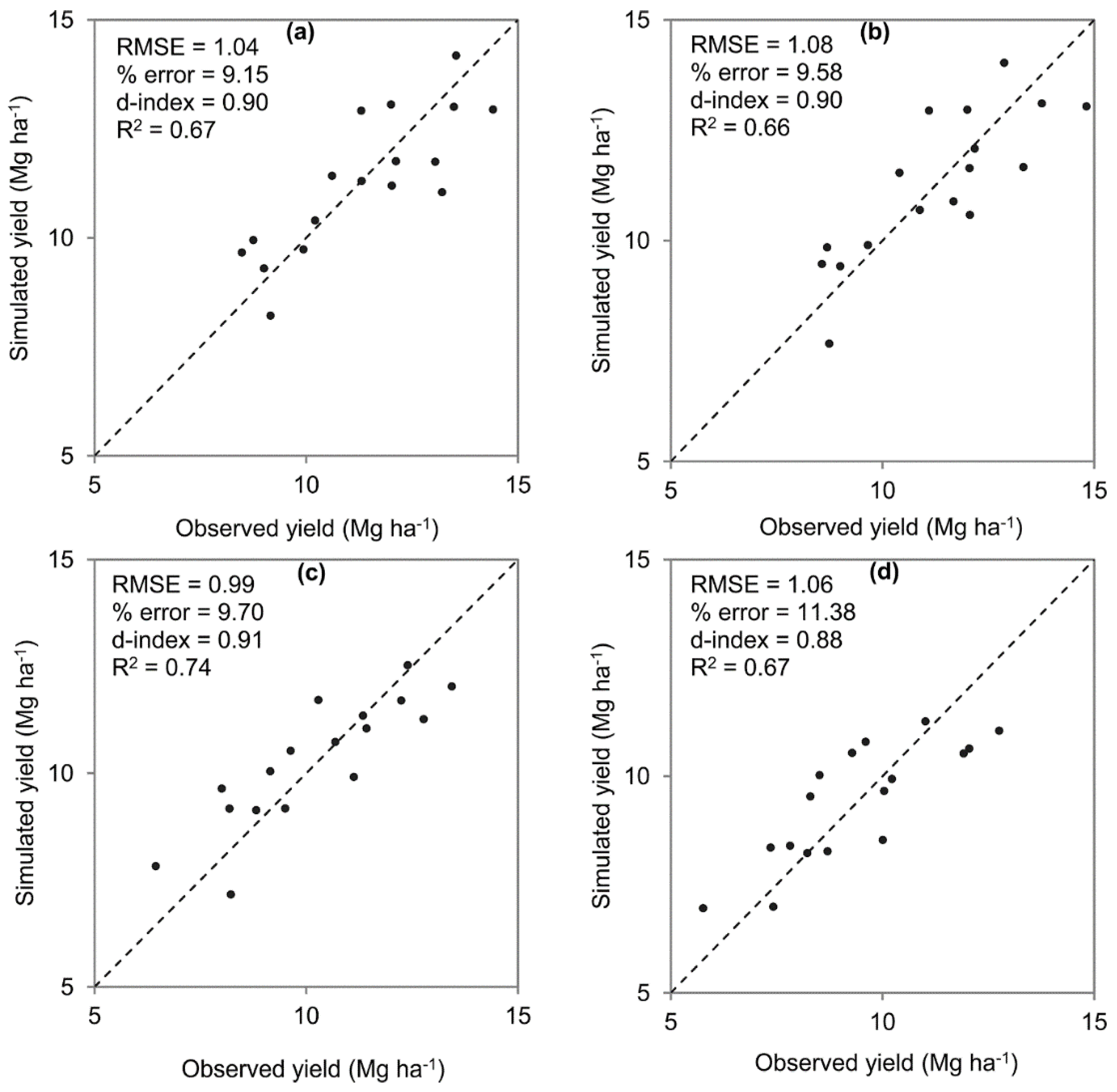
The statistics associated with the performance of the model while estimating the cultivar coefficients for each of the four cultivars is presented in Figure 3. The figure as well as the values of the goodness-of-fit measures used—RMSE, % error, R², and d-index—indicated that the performance of the CERES-Maize model was satisfactory. The model-simulated yields agreed with the observed yields (MSUES; http://msucares.com/pubs/crops3.html#grain) reasonably well.

Figure 3. The CERES-Maize-simulated vs. observed grain yields of maize (Mg·ha⁻¹) in the Mississippi Delta for cultivar: (a) AvTop5; (b) DynaGro-High; (c) DynaGro-Mid; and (d) DynaGro-Low.

Figure 3. The CERES-Maize-simulated vs. observed grain yields of maize (Mg·ha⁻¹) in the Mississippi Delta for cultivar: (a) AvTop5; (b) DynaGro-High; (c) DynaGro-Mid; and (d) DynaGro-Low.

3.2. Cultivar Effect

For all locations, the NEV values of cultivars AvTop5 and DynaGro-High did not vary from each other as they belonged to the same class, high-yielders, but varied from those of DynaGro-Mid and DynaGro-Low which were different from each other as they belonged to two different groups, mid-yielders and low-yielders, respectively (Table 5 and Figure 4). For all locations, the NEV values of DynaGro-High were highest and those of DynaGro-Low lowest as they were from high-yielders and low-yielders, respectively. The CCB had the same patterns as the NEV (Figure 4) because the latter was linearly associated with the former as: CCB = 0.2218NEV + 0.0477, where CCB is in credits·ha⁻¹ and NEV in GJ·ha⁻¹.

Table 5. Mean net energy values (NEV: GJ·ha⁻¹) associated with various factors and treatments at three locations in the Mississippi Delta. This table is summarized in Figure 4 for easier interpretation.

Factor	Treatment	Location
		Tunica	Moorhead	Vicksburg
Soil	Sandy loam	†B24.80c §	C24.22c	A30.27a
	Silty loam	A26.79a	A26.58a	A26.77c
	Silty clay loam	B25.04b	B25.51b	A28.24b
Cultivar	AvTop5	B26.94a	B27.06a	A30.97a
	DynaGro-High	B27.16a	B27.27a	A30.90a
	DynaGro-Mid	B25.11b	B24.87b	A27.28b
	DynaGro-Low	B22.97c	B22.64c	A24.60c
Irrigation (dry year)	No	B24.46c	B23.43b	A30.85b
	Light	B29.22a	C25.34a	A33.60a
	Moderate	B29.49a	C25.39a	A33.75a
	Heavy	B29.40a	C24.66a	A33.42a
	Extreme	B27.12b	C22.77b	A30.16b
Irrigation (wet year)	No	A20.36b	B15.09a	A22.37a
	Light	A23.23a	B15.09a	A22.37a
	Moderate	A22.69a	B15.10a	A21.87a
	Heavy	A22.70a	C14.69a	B20.96a
	Extreme	A20.80b	C10.38b	B17.40b
Irrigation (average year)	No	B25.34c	B25.27c	A28.80b
	Light	B26.60a	B26.47a	A29.63a
	Moderate	B26.53a	B26.36a	A29.55a
	Heavy	B25.99b	B25.78b	A28.99b
	Extreme	B23.26d	B23.29d	A25.22c

Notes: ^† Means preceded by the same upper case letter across locations within a treatment of a factor (horizontally) are not significantly different at p < 0.05 by the Tukey-Kramer LSD test; ^§ Means followed by the same lower case letter across treatments of a factor within a location (vertically) are not significantly different at p < 0.05 by the Tukey-Kramer LSD test.

Table 5. Mean net energy values (NEV: GJ·ha⁻¹) associated with various factors and treatments at three locations in the Mississippi Delta. This table is summarized in Figure 4 for easier interpretation.

Factor	Treatment	Location
		Tunica	Moorhead	Vicksburg
Soil	Sandy loam	†B24.80c §	C24.22c	A30.27a
	Silty loam	A26.79a	A26.58a	A26.77c
	Silty clay loam	B25.04b	B25.51b	A28.24b
Cultivar	AvTop5	B26.94a	B27.06a	A30.97a
	DynaGro-High	B27.16a	B27.27a	A30.90a
	DynaGro-Mid	B25.11b	B24.87b	A27.28b
	DynaGro-Low	B22.97c	B22.64c	A24.60c
Irrigation (dry year)	No	B24.46c	B23.43b	A30.85b
	Light	B29.22a	C25.34a	A33.60a
	Moderate	B29.49a	C25.39a	A33.75a
	Heavy	B29.40a	C24.66a	A33.42a
	Extreme	B27.12b	C22.77b	A30.16b
Irrigation (wet year)	No	A20.36b	B15.09a	A22.37a
	Light	A23.23a	B15.09a	A22.37a
	Moderate	A22.69a	B15.10a	A21.87a
	Heavy	A22.70a	C14.69a	B20.96a
	Extreme	A20.80b	C10.38b	B17.40b
Irrigation (average year)	No	B25.34c	B25.27c	A28.80b
	Light	B26.60a	B26.47a	A29.63a
	Moderate	B26.53a	B26.36a	A29.55a
	Heavy	B25.99b	B25.78b	A28.99b
	Extreme	B23.26d	B23.29d	A25.22c

Notes: ^† Means preceded by the same upper case letter across locations within a treatment of a factor (horizontally) are not significantly different at p < 0.05 by the Tukey-Kramer LSD test; ^§ Means followed by the same lower case letter across treatments of a factor within a location (vertically) are not significantly different at p < 0.05 by the Tukey-Kramer LSD test.

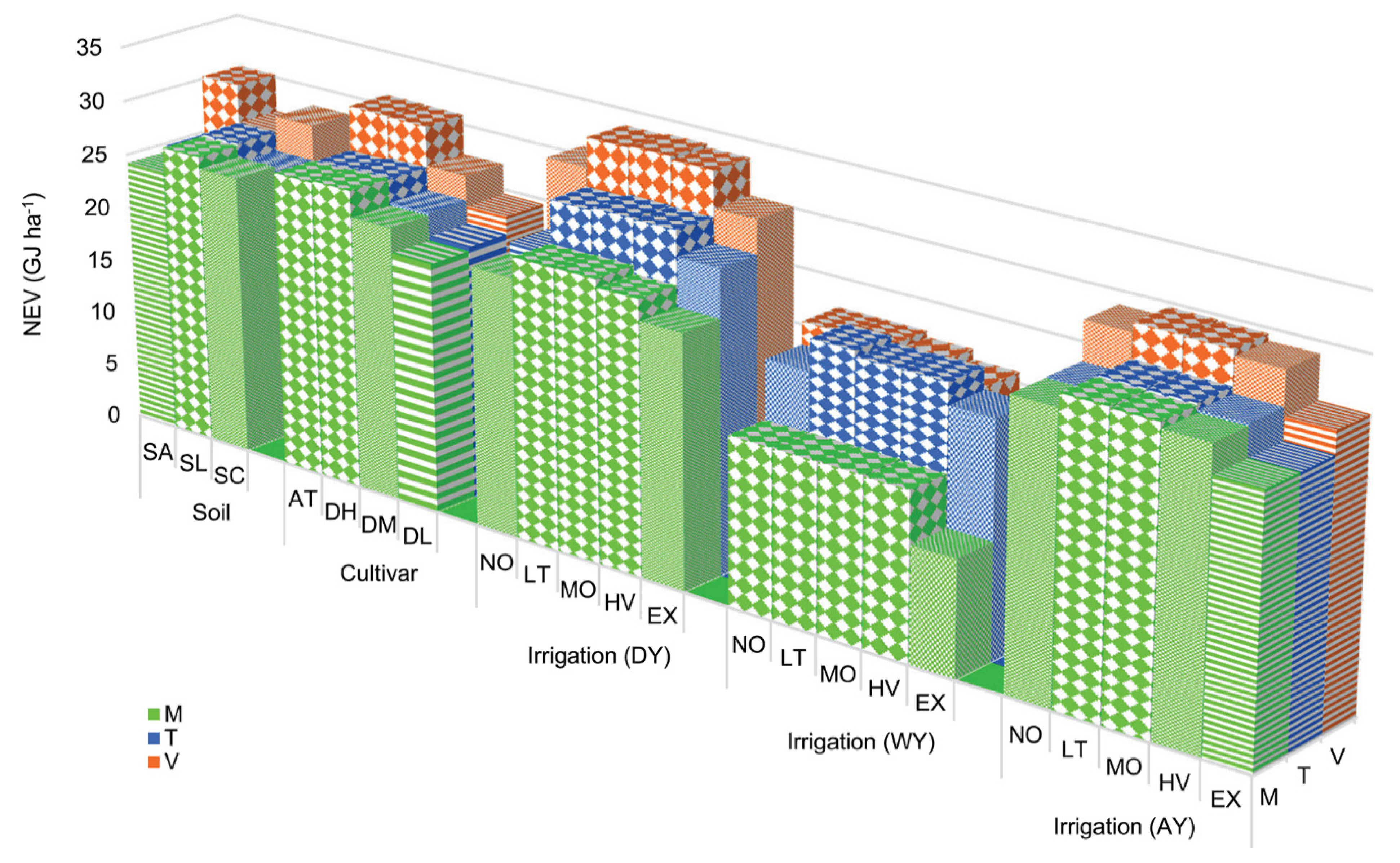
The NEV and CCB values of each cultivar in Vicksburg were greater than those in the other locations due to its larger root zone depth (RZD) and higher water holding capacity (WHC) (Table 1). The soil profile of larger RZD with higher WHC held more plant-available water in the soil for a longer period of time, thus leading to higher stover yields and ultimately greater NEV and CCB values. Although the average root zone in Tunica was deeper (169 cm) than that in Moorhead (152 cm), the average WHC of the former was lower (0.16) than that of the latter (0.18). Thus, no difference in NEV as well as CCB was found between these two locations for all cultivars.

Figure 4. Mean net energy values (NEV: GJ·ha⁻¹) for various factors, treatments, and locations. Values represented by the bars of the same color pattern across the treatments of a factor within a location are not significantly different, whereas those represented by the bars of different patterns are different from each other. For instance, the cultivars AT and DH for Moorhead (green bars) are not different from each other but are so from DM and DL which are different from each other. Abbreviations: SA = sandy loam, SL = silt loam, SC = silty clay loam, AT = average top 5, DH = DyanGro-High, DM = DynaGro-Mid, DL = Dynagro-Low, NO = no, LT = light, MO = moderate, HV = heavy, EX = extreme, M = Meadville, T = Tunica, V = Vicksburg, DY = dry year, WY = wet year, and AY = average year.

Figure 4. Mean net energy values (NEV: GJ·ha⁻¹) for various factors, treatments, and locations. Values represented by the bars of the same color pattern across the treatments of a factor within a location are not significantly different, whereas those represented by the bars of different patterns are different from each other. For instance, the cultivars AT and DH for Moorhead (green bars) are not different from each other but are so from DM and DL which are different from each other. Abbreviations: SA = sandy loam, SL = silt loam, SC = silty clay loam, AT = average top 5, DH = DyanGro-High, DM = DynaGro-Mid, DL = Dynagro-Low, NO = no, LT = light, MO = moderate, HV = heavy, EX = extreme, M = Meadville, T = Tunica, V = Vicksburg, DY = dry year, WY = wet year, and AY = average year.

3.3. Irrigation Effect

In general, NEV and CCB each showed a sigmoid relationship with the amount of irrigation applied. The NEV and CCB responses varied with weather conditions (Table 5 and Figure 4). Under dry conditions, the NEV and CCB values associated with light, moderate, and heavy irrigations were larger than those with no and extreme irrigations, but were not different among themselves for all locations. The difference in NEV as well as CCB with no irrigation was because soil never remained dry with light, moderate, and heavy irrigations as at least 25% of the field capacity was always maintained. Because soil water content even with light irrigation was nearly enough to sustain basic plant physiological processes, it did not vary across light, moderate, and heavy irrigations. Larger irrigation amounts did add additional water to the soil, but the marginal utilities of the added waters were not larger. The NEV and CCB values associated with no and extreme irrigations were smaller than those with light, moderate, and heavy irrigations because of drought and flooding, respectively. No and extreme irrigations had about the same values of NEV as well as CCB for Moorhead and Vicksburg, but different values for Tunica due to variation in minimum precipitation (out of 720 scenarios) during growing seasons. The minimum precipitation in Moorhead and Vicksburg was about the same, 170 and 155 mm, respectively, whereas that in Tunica, 231 mm, was significantly larger. Under dry conditions, larger precipitation led to more plant-available water, higher yields, and thus larger values of both NEV and CCB. For each irrigation treatment, values of NEV as well as CCB were different across locations due to variations in the RZD and WHC of their soils. In general, the NEV and CCB values increased in the order of Moorhead, Tunica, and Vicksburg for all irrigation treatments due to differences in RZD and WHC. The average values of RZD and WHC, respectively, were 152 cm and 0.16 for Moorhead, 170 cm and 0.18 for Tunica, and 187 cm and 0.21 for Vicksburg.

Under wet conditions, the values of both NEV and CCB associated with light, moderate, and heavy irrigations were not different from each other in all locations because irrigation did not significantly contribute to plant-available water as a large amount of water was already present in the soil. The NEV and CCB values associated with light, moderate, and heavy irrigations were larger than those with no and extreme irrigations in Tunica, but only with extreme irrigation in Moorhead and Vicksburg. The difference with no irrigation in Tunica was due to smaller precipitation. Because of high water content already in the soil due to large precipitation, the no irrigation could raise further the yields and thus the NEV as well as CCB values in Moorhead and Vicksburg. Instead, the increased irrigation amounts reduced yields and thus NEV and CCB values due to flooding. The NEV and CCB values associated with no and extreme irrigations were about the same in Tunica, but different in Moorhead and Vicksburg each due to precipitation differences (Tunica: 573 mm, Moorhead: 858 mm, Vicksburg: 853 mm). Because of large precipitation, the NEV and CCB values in Moorhead and Vicksburg fell down even below rainfed level due to excessive flooding. In Tunica, however, they did plunge significantly below rainfed level because of relatively less precipitation and flooding. At low irrigation levels (no, light, and moderate), the NEV and CCB values in Moorhead were smaller than those in Tunica and Vicksburg, which were about the same, but at high irrigation levels (heavy and extreme), the NEV and CCB values were different across locations. The smaller values of NEV and CCB in Moorhead were due to larger precipitation and shallower root zone (152 cm) and thus more water logging. Vicksburg had about the same precipitation, but its root zone was deeper (203 cm) so its root zone did not saturate as quickly as that of Moorhead and the NEV and CCB values did not plunge much. The difference across locations with heavy and extreme irrigations was because at these irrigation treatments even the deepest layer of Vicksburg got nearly saturated, causing yields and thus NEV and CCB values to decline further.

Under average conditions, values of both NEV and CCB associated with light and moderate irrigations were the largest of all irrigation treatments for all locations due to optimum soil moisture conditions. For the same reason, the NEV and CCB values associated with light and moderate irrigations were about the same. Values of NEV as well as CCB associated with extreme irrigation were lowest for all locations because of excessive irrigation and frequent flooding. The NEV and CCB values associated with heavy irrigation were larger than those with no irrigation due to less water deficit, but smaller than those with light and moderate irrigations due to more waterlogging. For all irrigation treatments, the NEV and CCB values in Vicksburg were larger than those in Tunica and Moorhead whereby values were about the same. The larger values of both NEV and CCB in Vicksburg were mainly due to its larger RZD and higher WHC.

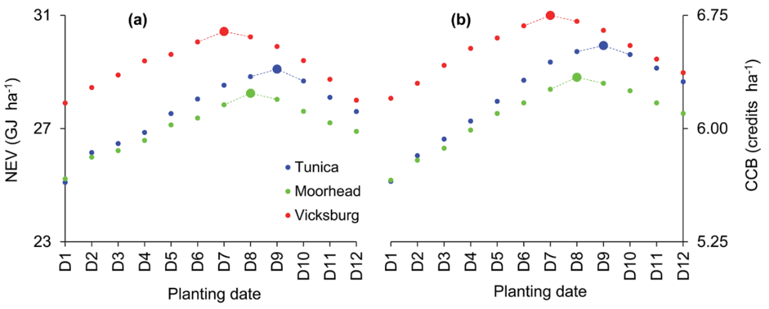
3.4. Planting Date Effect

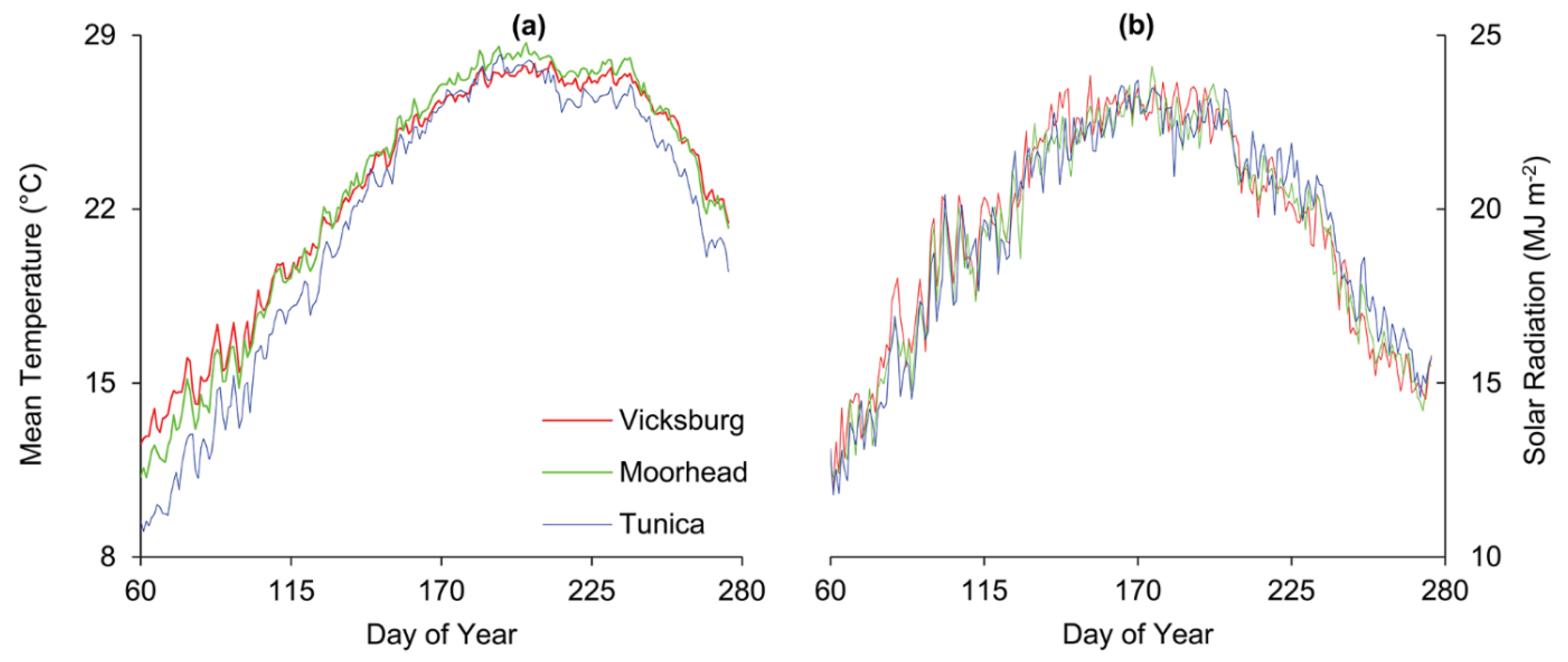
Both NEV and CCB increased with a delay in planting date until the middle part of the planting window, peaked at 18 April for Vicksburg, 25 April for Moorhead, and 4 May for Tunica, and declined thereafter (Figure 5). Such responses were due to temperature and solar radiation, both of which increased quickly in the beginning but slowly later in the season (Figure 1). While the rate of temperature increase affected the rates of plant physiological activities and development, the rate of solar radiation affected the rates of photosynthesis and plant growth. When day temperatures reached above favorable temperature range, crop growth and development rates decreased considerably, causing the NEV and CCB values to fall.

Figure 5. Planting date effect on: (a) net energy value (NEV) and (b) carbon credit balance (CCB) at three locations in the Mississippi Delta. The largest marker for each location in each panel indicates the largest value of the response variable and the associated optimum planting date. Values connected by dashed lines were not significantly different (p < 0.05) from the largest value for the given location. Planting dates: D1 = 4 March, D2 = 11 March, D3 = 18 March, D4 = 25 March, D5 = 4 April, D6 = 11 April, D7 = 18 April, D8 = 25 April, D9 = 4 May, D10 = 11 May, D11 = 18 May, and D12 = 25 May.

Figure 5. Planting date effect on: (a) net energy value (NEV) and (b) carbon credit balance (CCB) at three locations in the Mississippi Delta. The largest marker for each location in each panel indicates the largest value of the response variable and the associated optimum planting date. Values connected by dashed lines were not significantly different (p < 0.05) from the largest value for the given location. Planting dates: D1 = 4 March, D2 = 11 March, D3 = 18 March, D4 = 25 March, D5 = 4 April, D6 = 11 April, D7 = 18 April, D8 = 25 April, D9 = 4 May, D10 = 11 May, D11 = 18 May, and D12 = 25 May.

Although the overall response of NEV and CCB each to planting date was the same across locations, values of both NEV and CCB and the optimum planting dates/windows were different. For Moorhead and Tunica, the NEV/CCB values associated with initial planting dates (in March) were about the same because the amount of solar radiation in these locations during this period was also the same (Figure 1b). During the mid and terminal parts of the planting window, however, the values for Tunica were larger than those for Moorhead due to the difference in solar radiation. Values of NEV/CCB in Vicksburg were the largest of all locations for all planting dates. However, due to decreasing differences in both temperature and solar radiation, the NEV/CCB gaps between Vicksburg and Tunica decreased almost linearly until the planting date reached peak values. Values of temperature and solar radiation in Vicksburg were always larger than those in Tunica throughout the first half of the crop growing season, but with a linear decrease in the gap. During the second half of the season, however, values of solar radiation in Tunica were always larger than those in Vicksburg. The larger values of NEV/CCB in Vicksburg than in Tunica even at the terminal part of the planting window were due to more radiation during initial vegetative phase. The decline in NEV/CCB values thereafter was due to high temperatures.

Due to daily rise in solar radiation and temperature in the northern hemisphere during spring and summer seasons, values of NEV and CCB increased for every delay in planting until an optimum planting date (associated with the highest yield) was reached. The NEV and CCB values associated with planting dates after the optimum date declined due to temperatures too high to optimal plant growth. Because in a particular day or period locations at lower latitudes get warmer earlier, Vicksburg (32.36° N) attained the optimum planting date earlier (18 April) than the other locations. The NEV and CCB values associated with planting dates after 18 April kept declining as daily maximum temperature entered suboptimal zone, thus hampering germination and early crop development. Moorhead (33.45° N) and Tunica (34.68° N) approached the peak values with the planting dates of 25 April and 4 May, respectively, after which they entered the suboptimal temperature zone.

For Vicksburg, the NEV and CCB values associated with planting dates 11 April, 18 April, and 25 April were not significantly different from those associated with 18 April, the optimum planting date, indicating 11–25 April as the optimum planting window for this location (Figure 5). Similarly, the optimum planting windows for Moorhead and Tunica were found to be the periods of 18 April through 7 May and 25 April through 11 May. With a northward shift in location from Vicksburg to Moorhead to Tunica, the optimum planting window shifted forward by a week.

3.5. Soil Effect

The values of NEV as well as CCB associated with the three soils were different from each other for all locations (Table 5 and Figure 4) due to variation in soil properties (Table 1). The order of difference among the soils, however, was different across locations. While silt loam was the largest producer of stover yields and thus was associated with the largest values of both NEV and CCB for Tunica and Moorhead, sandy loam produced the most and provided the largest values for Vicksburg. Among the three soils, the smallest values of NEV and CCB for Tunica and Moorhead were associated with sandy loam and those for Vicksburg with silt loam. The largest and smallest NEV/CCB values associated with silt loam and sandy loam for Tunica were due to its highest and lowest WHCs, respectively. The largest, intermediate, and smallest NEV/CCB values associated with silt loam, silty clay loam, and sandy loam for Moorhead were due to, respectively, the largest, intermediate, and smallest values of WHC, soil organic carbon content (SOC), and cation exchange capacity (CEC) each. For Vicksburg, sandy loam was associated with the largest NEV/CCB values due to its highest WHC and deepest root zone and silt loam with the smallest values due to its shallowest root zone and relatively lower WHC. Silty clay loam had smaller NEV/CCB values than sandy loam due to its smaller WHC, SOC, and CEC values, but larger NEV/CCB values than silt loam due to its deeper root zone and larger values of SOC and SEC.

The NEV and CCB values associated with sandy loam were different across locations. The sandy loam-related values were largest for Vicksburg due to its highest WHC and deeper root zone and smallest for Moorhead due to its shallowest root zone and smallest CEC and SOC values. The NEV and CCB values in Tunica were intermediate due to its intermediate RZD, WHC, CEC, and SOC values. For silt loam-associated values, no location was different from the others because of similar soil properties. For silty clay loam-related values, only Vicksburg was different due to its highest WHC and deepest root zone. Moorhead and Tunica did not vary from each other because of similar soil properties.

3.6. Interaction Effect

To examine the interaction effects of the four factors, the factor combinations associated with the largest and smallest values of NEV and CCB were chosen out of the total 720 scenarios and analyzed for each location and each of the three weather conditions. Under dry condition, values of both NEV and CCB increased by 121%, 126%, and 257% for Tunica, Vicksburg, and Moorhead, respectively, when moved from the lowest to the highest value scenario (Table 6). Under wet condition, the increase was 279%, 297%, and 552% for Tunica, Vicksburg, and Moorhead, respectively. Under average weather condition, values of both NEV and CCB increased by 416%, 665%, and 690% for Vicksburg, Moorhead, and Tunica, respectively. For shifts from dry to wet, dry to average, and wet to average conditions, the gaps widened by 2.1 to 2.4, 2.6 to 5.7, and 1.2 to 2.5 folds, respectively, depending on location.

Table 6. Values of net energy (NEV: GJ·ha⁻¹) and carbon credit balance (CCB: credits·ha⁻¹) under highest and lowest production situations for dry, average, and wet years at three locations.

Scenario		Tunica			Moorhead			Vicksburg
		Combination	NEV	CCB	Combination	NEV	CCB	Combination	NEV	CCB
Dry year	Lowest	C4-I1-D8-S1 a	38	8	C4-I5-D1-S1	24	5	C4-I5-D12-S3	44	9
	Highest	C2-I5-D5-S1	85	18	C2-I5-D10-S2	85	18	C1-I3-D2-S3	99	21
	PI b	-	121	121	-	257	257	-	126	126
Wet year	Lowest	C4-I3-D3-S1	22	5	C4-I5-D5-S1	13	3	C4-I5-D3-S2	21	5
	Highest	C2-I5-D13-S1	83	18	C2-I4-D12-S2	82	18	C1-I1-D8-S3	84	18
	PI	-	279	279	-	552	552	-	297	297
Av. year	Lowest	C4-I1-D12-S1	12	3	C4-I5-D5-S1	13	3	C4-I5-D2-S2	21	5
	Highest	C2-I4-D1-S1	97	21	C2-I1-D12-S3	96	21	C1-I5-D6-S1	108	23
	PI	-	690	690	-	665	665	-	416	416

Notes: ^a C4-I1-D8-S1: The scenario of C4, I1, D8, and S1. C1 = AvTop5, C2 = DynaGro-High; C4 = DynaGro-Low; I1 = no irrigation; I3 = moderate irrigation; I4 = heavy irrigation; I5 = extreme irrigation; D1 = 4 March; D2 = 11 March; D3 = 18 March; D4 = 25 March; D5 = 4 April; D6 = 11 April; D8 = 25 April; D10 = 11 May; D12 = 25 May; S1 = sandy loam; S2 = silt loam; S3 = silty clay loam; ^b PI = Percent increase from the lowest to the highest scenario = 100(highest – lowest)/lowest.

Table 6. Values of net energy (NEV: GJ·ha⁻¹) and carbon credit balance (CCB: credits·ha⁻¹) under highest and lowest production situations for dry, average, and wet years at three locations.

Scenario		Tunica			Moorhead			Vicksburg
		Combination	NEV	CCB	Combination	NEV	CCB	Combination	NEV	CCB
Dry year	Lowest	C4-I1-D8-S1 a	38	8	C4-I5-D1-S1	24	5	C4-I5-D12-S3	44	9
	Highest	C2-I5-D5-S1	85	18	C2-I5-D10-S2	85	18	C1-I3-D2-S3	99	21
	PI b	-	121	121	-	257	257	-	126	126
Wet year	Lowest	C4-I3-D3-S1	22	5	C4-I5-D5-S1	13	3	C4-I5-D3-S2	21	5
	Highest	C2-I5-D13-S1	83	18	C2-I4-D12-S2	82	18	C1-I1-D8-S3	84	18
	PI	-	279	279	-	552	552	-	297	297
Av. year	Lowest	C4-I1-D12-S1	12	3	C4-I5-D5-S1	13	3	C4-I5-D2-S2	21	5
	Highest	C2-I4-D1-S1	97	21	C2-I1-D12-S3	96	21	C1-I5-D6-S1	108	23
	PI	-	690	690	-	665	665	-	416	416

Notes: ^a C4-I1-D8-S1: The scenario of C4, I1, D8, and S1. C1 = AvTop5, C2 = DynaGro-High; C4 = DynaGro-Low; I1 = no irrigation; I3 = moderate irrigation; I4 = heavy irrigation; I5 = extreme irrigation; D1 = 4 March; D2 = 11 March; D3 = 18 March; D4 = 25 March; D5 = 4 April; D6 = 11 April; D8 = 25 April; D10 = 11 May; D12 = 25 May; S1 = sandy loam; S2 = silt loam; S3 = silty clay loam; ^b PI = Percent increase from the lowest to the highest scenario = 100(highest – lowest)/lowest.

The factor combinations associated with the lowest and highest scenarios under the three weather conditions did not show any specific pattern due to interactions among the factors (Table 6). For each location, the interaction effects were significant for most of the 2-, 3-, and 4-factor interactions. The insignificant interactions were very few and varied by location due to differences in root zone depth and water holding capacity.

3.7. Travel Distance Effect

The values of NEV and CCB estimated in terms of per Mg stover used for ethanol production and per m³ ethanol produced for three locations in the Mississippi Delta are presented in Table 7. The figures in the table show that travel distance has negative influence on NEV_s, NEV_e, CCB_s, and CCB_e. The values of these variables decreased in the order of Vicksburg, Moorhead, and Tunica because the travel distance increased in the same order. Although the NEV/CCB variables decreased with an increase in travel distance, they did not vary significantly across locations due to little contribution of transportation relative to those of the other activities in the biomass supply chain combined (Equations (2) and (4)). The insignificant difference was also because the travel distance difference across locations was not significantly large. Even though the differences were not very significant, the results at least gave an impression that the energy and emission costs of stover-based ethanol production would increase with an increase in travel distance.

Table 7. Net energy value (NEV) and carbon credit balance (CCB) as influenced by travel distance for three locations in the Mississippi Delta.

Variable a		Unit	Location
			Vicksburg	Moorhead	Tunica
Travel distance (D)		km	90	145	160
NEV	NEVs	GJ·Mg−1	6.29	6.19	6.17
	NEVe	GJ·m−3	20.96	20.65	20.56
CCB	CCBs	credits·Mg−1	1.397	1.390	1.388
	CCBe	credits·m−3	4.656	4.632	4.625

Notes: ^a NEV_s = NEV on per Mg stover basis; NEV_e = NEV on per m³ ethanol basis; CCB_s = CCB on per Mg stover basis; CCB_e = CCB on per m³ ethanol basis.

Table 7. Net energy value (NEV) and carbon credit balance (CCB) as influenced by travel distance for three locations in the Mississippi Delta.

Variable a		Unit	Location
			Vicksburg	Moorhead	Tunica
Travel distance (D)		km	90	145	160
NEV	NEVs	GJ·Mg−1	6.29	6.19	6.17
	NEVe	GJ·m−3	20.96	20.65	20.56
CCB	CCBs	credits·Mg−1	1.397	1.390	1.388
	CCBe	credits·m−3	4.656	4.632	4.625

Notes: ^a NEV_s = NEV on per Mg stover basis; NEV_e = NEV on per m³ ethanol basis; CCB_s = CCB on per Mg stover basis; CCB_e = CCB on per m³ ethanol basis.

4. Discussion

This study demonstrated that different soils in combination with different cultivars, planting dates, and irrigation amounts change the NEV and CCB of maize stover-based ethanol production. This study is different from the previous ones that examined biofuel production systems, such as Shapouri et al. [23], Kim and Dale [59], Hill et al. [70], and Pradhan et al. [71], in that not only did it analyze ethanol production from NEV and CCB perspectives but also explicitly accounted for the effects of variability in cultivar, irrigation level, planting date, and soil type using a modeling approach.

This study showed that cultivar can significantly affect the NEV and CCB of stover-based ethanol production for the Mississippi Delta, which is in agreement with the results of Persson et al. [30] and Woli et al. [20]. Persson et al. [30] compared three maize hybrids in Georgia and found NEV to be significantly different across cultivars. Woli et al. [20] demonstrated that the CCB and NEV of switchgrass-based ethanol production systems in Mississippi could be increased with alternative soil and cultivar options.

As this study showed, variation in irrigation levels could significantly change the values of NEV and CCB. Persson et al. [22,32] also found similar results for the NEV associated with maize grain-based ethanol production for Georgia. The positive effects of irrigation on NEV and CCB were due to increased stover yields. Woli and Paz [21] found that the sustainability and eco-friendliness of ethanol production associated with maize-stover and switchgrass would increase with an increase in yield level and utilization rate. Under all the three weather conditions, extreme irrigation produced the lowest yields and thus the smallest values of NEV and CCB, and light and moderate irrigations produced the largest values. Under dry conditions, light, moderate, and heavy irrigations produced the largest values of NEV and CCB. Under wet conditions, however, no effect of irrigation on these variables was found, except for extreme irrigation. The differences in NEV and CCB among irrigation treatments, however, are valid under the assumption that the energy and emissions costs of irrigation are applied to grain, not stover, a by-product of grain production.

This study also demonstrated that planting date has significant effects on NEV and CCB, and that these variables can be maximized by planting the crop during the optimum planting window of 11–25 April for Vicksburg, 18 April through 7 May for Moorhead, and 25 April through 11 May for Tunica. Persson et al. [22] also found that delayed planting increased maize yields, but the differences among the three planting dates they compared (3, 17, and 31 March) were not large. The optimum planting windows estimated in our study did not match with those suggested by the Mississippi State University Extension Service: 5 March through 10 April for Vicksburg, 15 March through 20 April for Moorhead, and 20 March through 25 April for Tunica [36]. The suggested windows are based on maintaining soil temperature at 10–13 °C at the beginning of planting season, avoiding the outbreak of insects and diseases later in the season through early crop development, and avoiding water and temperature stresses during peak growing period, which generally occurs in July and August if planted late. These suggestions are for all years and all cultivars in general. Our estimates, on the other hand, are based on weather-specific simulations. Moreover, the MSUES-suggested dates are for typical cultivars, whereas our estimated dates are based on new hybrids. In southeastern USA, maize can be planted from late February through early July, and summer rainfall is often more favorable for the crop planted from mid-May to mid-June [37]. Maize hybrids that are being developed from tropical germplasm are adapted to the summer rainfall pattern in this region [72]. However, planting is generally terminated by early May due to severe insect pressure later in the season [37]. Because our study represented only standard production conditions (no occurrence of pest and disease assumed), the estimated optimum planting windows were defined mainly by genotype and weather variables. Thus, these estimates are mainly applicable to standard production conditions. Because planting date is a function of cultivar (genotype) and new cultivars evolve every year, determining the optimum planting date for every new cultivar through research is necessary. Our estimates may be taken as a starting point for new hybrids.

The results of this study indicated that soils with deeper root zones and larger values of WHC, CEC, and SOC can produce larger values of NEV and CCB. Persson et al. [32] also observed that larger values of NEV were associated with soils with higher WHC.

The NEV and CCB values were found to increase with an increase in stover yield, but to decrease with an increase in travel distance. However, the influence of stover yield on NEV and CCB was found to have been far more than that of travel distance because the latter affected only transportation costs, whereas the former affected the costs of all activities in the feedstock supply chain [24]. The ratio of CO₂ emitted to CO₂ fixed was 0.071 for Vicksburg, 0.076 for Moorhead, and 0.077 for Tunica. That is, the overall ratio of CO₂ emitted to stover yield in the Mississippi Delta was about 0.0001. These results indicated that increasing feedstock yields should get more emphasis [73] relative to decreasing travel distance or decreasing the emissions from feedstock transportation although both are important. Macedo et al. [74] also found similar results for sugarcane-based ethanol production systems in Brazil.

This study showed, in terms of NEV and CCB, respectively, that the sustainability and eco-friendliness of maize stover-based ethanol production in the Mississippi Delta could be increased with alternative cultivar, irrigation, and planting date options. The location-specific information on the responses of NEV and CCB to these options might be helpful to maize stover producers and biorefineries in this region in promoting the sustainability (in terms of non-renewable energy displacement) and eco-friendliness (in terms of carbon emissions reduction) of ethanol production. Farming practices increasing NEV and CCB might be promoted through various measures, policies, and programs such as consumer awareness [75], government support [76,77,78], and personal carbon trading [79,80].

The factors and variables considered in this study represented only simplified conditions. For simplicity, other crop management variables such as fertilization, plant protection, and tillage were assumed to be fixed and in standard conditions. For instance, soils were assumed to be fertile, and crops were assumed to be well protected from pests and diseases. In reality, however, these conditions might vary over time and space. Removing stover from the production field might promote soil erosion, deplete soil carbon, and reduce the return of nutrients to the soil. For the ethanol production system considered in this study, the removal rate that would keep soil erosion within tolerable soil-loss limit and would also not let soil carbon level deplete was assumed to be 40% [60]. This removal rate, however, applies only to a region having nearly level ground and continuous maize production with mulch-till system. For the other regions that are different from the one considered in this study, this removal rate might promote soil erosion and carbon depletion. For the other systems, therefore, this removal rate may not be applicable. The stover removal rate even with tolerable soil-loss limit removes some nutrients from the soil. In this study, however, the nutrient replacement cost was not considered for stover, a by-product of maize grain production. If stover production also is an objective of growing maize, the nutrient replacement cost must be considered for stover. Assuming stover as a free material (by-product), the energy use and CO₂ emissions associated with stover production for producing or applying various inputs were not included in analyses [66]. In the systems that do not consider stover a free material, however, the energy used and CO₂ emitted during input production and application must also be accounted for. The optimum planting dates or windows determined for the three locations were based on average yields of 30 years, that is, 30 replications. For other replication numbers, the results could be different because of annual climate variability. The optimum planting dates might fluctuate more with fewer replications, but could be more robust with more replications. In our study, the weather data of the 1971–2000 normal period was used, considering the three-decade interval as long enough to filter out many of the short-term inter-annual fluctuations and anomalies and short enough to reflect long-term climatic trends [81]. Our study computed CCB only for the production side of ethanol, that is, for supplying a given quantity of stover to a biorefinery and processing it. The CO₂ emissions associated with distribution and combustion of ethanol were beyond the scope of this study.

This work may be regarded as an example of studying the effects of soil, cultivar, and management on the NEV and CCB of ethanol from crop residues and other lignocellulosic resources. The effects of these variables on other feedstocks may be studied applying the methodology used in this study. To provide a broader perspective of soil, cultivar, and management effects on greenhouse gas (GHG) emissions, additional GHGs such as methane and nitrous oxide may be considered [60]. The approach of our study might be expanded to other maize production areas of Mississippi or other maize growing states such as the Corn Belt. This study considered travel distance as fixed assuming the production area as small. As travel distance is influenced by several factors such as crop yield, production area, and refinery capacity [82], computing NEV and CCB as a function of varying travel distance may be a consideration for a future study. The objective of this study was to identify the agronomic conditions—the combinations of cultivar, irrigation, planting date, and soil—that would maximize the NEV and CCB of the ethanol production systems under the contemporary set of farm and refinery technologies, so a fixed set of energy and emission values were used in this study. If the objective were also to identify the engineering conditions—the combinations of various harvesting, baling, transportation, and processing technologies—the energy and emission constants would be parameters and thus have ranges of values. This study did not include the engineering aspects considering agricultural community using the contemporary set of technologies as the principal target audience; identifying engineering conditions that would maximize the NEV and CCB values, however, can be a potential subject matter for a separate future study targeted for a broader audience.

5. Conclusions

The results of this study showed that the NEV and CCB of maize stover-based ethanol production would vary significantly across soils and cultivars. Deeper soils with higher water holding capacity were found to have larger values of NEV and CCB. With an increase in irrigation and with every one-week delay in planting, the NEV and CCB values increased at first but decreased after reaching a peak. Planting date had significant effects on NEV and CCB, which could be maximized by planting the crop from 11 to 25 April for Vicksburg, 18 April to 7 May for Moorhead, and 25 April to 11 May for Tunica. Stover yield was found to have positive effects on NEV and CCB, whereas travel distance negative. The influence of stover yield was larger than that of travel distance, indicating that increasing feedstock yields should be emphasized over reducing travel distance. Values of NEV and CCB were positive for all scenarios, indicating that stover-based ethanol production in the Mississippi Delta is sustainable and environmentally friendly. The study demonstrated that the energy sustainability and eco-friendliness of maize stover-based ethanol production could be increased with alternative soil, cultivar, irrigation, and planting date options.

References

1. National Research Council. Review of the Research Strategy for Biomass-Derived Transportation Fuels; National Academy Press: Washington, DC, USA, 1999. [Google Scholar]
2. Smith, P.; Powlson, D.S.; Smith, J.U.; Falloon, P.; Coleman, K. Meeting Europe’s climate change commitments: Quantitative estimates of the potential for carbon mitigation by agriculture. Glob. Chang. Biol. 2000, 6, 525–539. [Google Scholar] [CrossRef]
3. McLaughlin, S.B.; de la Torre Ugarte, D.G.; Garten, T., Jr.; Lynd, L.R.; Sanderson, M.A.; Tolbert, V.R.; Wolf, D.D. High value renewable energy from prairie grasses. Environ. Sci. Technol. 2002, 36, 2122–2129. [Google Scholar] [CrossRef] [PubMed]
4. U.S. Department of Energy. Office of the Biomass Program: Multiyear Analysis Plan FY04-FY08. Available online: http://www.nrel.gov/docs/fy05osti/36999.pdf (accessed on 7 January 2014).
5. Tilman, D.; Socolow, R.; Foley, J.A.; Hill, J.; Larson, E.; Lynd, L.; Pacala, S.; Reilly, J.; Searchinger, T.; Somerville, C.; et al. Beneficial biofuels: The food, energy, and environment trilemma. Science 2009, 325, 270–271. [Google Scholar] [CrossRef] [PubMed]
6. Cherubini, F.; Jungmeier, G. LCA of biorefinery concept producing bioethanol, bioenergy, and chemicals from switchgrass. Int. J. Life Cycle Assess. 2010, 15, 53–66. [Google Scholar] [CrossRef]
7. Shields, S.; Boopathy, R. Ethanol production from lignocellulosic biomass of energy cane. Int. Biodeterior. Biodegrad. 2011, 65, 142–146. [Google Scholar] [CrossRef]
8. Giampietro, M.; Ulgiati, S.; Pimentel, D. Feasibility of large-scale biofuel production. Bioscience 1997, 47, 587–600. [Google Scholar] [CrossRef]
9. Gnansounou, E.; Dauriat, A. Techno-economic analysis of lignocellulosic ethanol: A review. Bioresour. Technol. 2010, 101, 4980–4991. [Google Scholar] [CrossRef] [PubMed]
10. Hammerschlag, R. Ethanol’s energy return on investment: A survey of the literature 1990–present. Environ. Sci. Technol. 2006, 40, 1744–1750. [Google Scholar] [CrossRef] [PubMed]
11. Fischer, G.; Prieler, S.; van Velthuizen, H.; Lensink, S.M.; Londo, M.; de Wit, M. Biofuel production potentials in Europe: Sustainable use of cultivated land and pastures. Part I: Land productivity potentials. Biomass Bioenergy 2010, 34, 159–172. [Google Scholar] [CrossRef]
12. Perlack, R.D.; Wright, L.L.; Turhollow, A.F.; Graham, R.L.; Stokes, B.J.; Erbach, D.C. Biomass as Feedstock for a Bioenergy and Bioproducts Industry: The Technical Feasibility of a Billion-Ton Annual Supply; U.S. Department of Agriculture (USDA)/U.S. Department of Energy (USDE): Washington, DC, USA, 2005. [Google Scholar]
13. Chandel, A.K.; Singh, O.V. Weedy lignocellulosic feedstock and microbial metabolic engineering: Advancing the generation of “Biofuel”. Appl. Microbiol. Biotechnol. 2011, 89, 1289–1303. [Google Scholar] [CrossRef] [PubMed]
14. Narayanaswamy, N.; Faik, A.; Goetz, D.J.; Gu, T. Supercritical carbon dioxide pretreatment of corn stover and switchgrass for lignocellulosic ethanol production. Bioresour. Technol. 2011, 102, 6995–7000. [Google Scholar] [CrossRef] [PubMed]
15. Dhugga, K.S. Maize biomass yield and composition for biofuels. Crop. Sci. 2007, 47, 2211–2227. [Google Scholar] [CrossRef]
16. Perlack, R.D.; Turhollow, A.F. Assessment of Options for the Collection, Handling, and Transport of Maize Stover; ORNL/TM-2002/44; Oak Ridge National Laboratory: Oak Ridge, TN, USA, 2002. [Google Scholar]
17. Qiu, C. Evaluating Biomass Feedstock Availability and Cost for Fueling Ethanol Production in South Dakota Counties. Master’s Thesis, South Dakota State University, Brookings, SD, USA, 2009. [Google Scholar]
18. Historic US Fuel Ethanol Production; Renewable Fuels Association (RFA): Washington, DC, USA, 2009. Available online: http://www.ethanolrfa.org/pages/statistics#A (accessed on 5 March 2014).
19. Fact Sheet: Energy Independence and Security Act 2007; United States Department of Energy (USDE): Washington, DC, USA, 2007.
20. Woli, P.; Paz, J.O.; Lang, D.J.; Baldwin, B.S.; Kiniry, J.R. Soil and variety effects on the energy and carbon balances of switchgrass-derived ethanol. J. Sustain. Bioenergy Syst. 2012, 2, 65–74. [Google Scholar] [CrossRef]
21. Woli, P.; Paz, J.O. Biomass yield and utilization rate effects on the sustainability and environment-friendliness of maize stover- and switchgrass-based ethanol production. Int. J. Environ. Bioenergy 2013, 7, 28–42. [Google Scholar]
22. Persson, T.; Garcia y Garcia, A.; Paz, J.O.; Jones, J.W.; Hoogenboom, G. Maize ethanol feedstock production and net energy value as affected by climate variability and crop management practices. Agric. Syst. 2009, 100, 11–21. [Google Scholar] [CrossRef]
23. Shapouri, H.; Duffield, J.A.; Wang, M. The Energy Balance of Maize Ethanol: An Update; Agricultural Economic Report 814; United States Department of Agriculture: Washington, DC, USA, 2002. [Google Scholar]
24. Sokhansanj, S.; Kumar, A.; Turhollow, A.F. Development and implementation of integrated biomass supply analysis and logistics model (IBSAL). Biomass Bioenergy 2006, 30, 838–347. [Google Scholar] [CrossRef]
25. Morey, R.V.; Kaliyan, N.; Tiffany, D.G.; Schmidt, D.R. A corn stover supply logistics system. Appl. Eng. Agric. 2010, 26, 455–461. [Google Scholar] [CrossRef]
26. Kheshgi, H.S.; Princes, R.C.; Marland, G. The potential of biomass fuels in the context of global climate change: Focus on transportation fuels. Annu. Rev. Energy Environ. 2000, 25, 199–244. [Google Scholar] [CrossRef]
27. Persson, T.; Ortiz, B.V.; Bransby, D.I.; Wu, W.; Hoogenboom, G. Determining the impact of climate and soil variability on switchgrass (Panicum virgatum L.) production in the south-eastern USA; A simulation study. Biofuels Bioprod. Biorefin. 2011, 5, 505–518. [Google Scholar] [CrossRef]
28. Eksioglu, S.D.; Acharya, A.; Leightley, L.E.; Arora, S. Analyzing the design and management of biomass-to-biorefinery supply chain. Comput. Ind. Eng. 2009, 57, 1342–1352. [Google Scholar] [CrossRef]
29. Data and Statistics; United States Department of Agriculture (USDA) National Agricultural Statistics Service: Washington, DC, USA, 2011. Available online: http://www.nass.usda.gov/Data_and_Statistics/Quick_Stats_1.0/index.asp#top (accessed on 9 November 2013).
30. Persson, T.; Garcia y Garcia, A.; Paz, J.O.; Ortiz, B.V.; Hoogenboom, G. Simulating the production potential and net energy yield of maize-ethanol in the southeastern USA. Eur. J. Agron. 2010, 32, 272–279. [Google Scholar] [CrossRef]
31. McLaughlin, S.B.; Kszos, L.A. Development of switchgrass (Panicum virgatum) as a bioenergy feedstock in the United States. Biomass Bioenergy 2005, 28, 515–535. [Google Scholar] [CrossRef]
32. Persson, T.; Garcia y Garcia, A.; Paz, J.O.; Jones, J.W.; Hoogenboom, G. Net energy value of maize ethanol as a response to different climate and soil conditions in the southeastern USA. Biomass Bioenergy 2009, 33, 1055–1064. [Google Scholar] [CrossRef]
33. Snipes, C.E.; Evans, L.P.; Poston, D.H.; Nichols, S.P. Agricultural practices of the Mississippi Delta. In Water Quality Assessments in the Mississippi Delta: Regional Solutions Scope (ACS Symposium Series 877); Nett, M.T., Locke, M.A., Pennington, D.A., Eds.; American Chemical Society: Washington, DC, USA, 2004; pp. 43–60. [Google Scholar]
34. Woli, P.; Paz, J.O. Evaluation of various methods for estimating global solar radiation in the southeastern USA. J. Appl. Meteorol. Climatol. 2012, 51, 972–985. [Google Scholar] [CrossRef]
35. Soil Data Access; United States Department of Agriculture (USDA) Natural Resources Conservation Service: Washington, DC, USA, 2014. Available online: http://msucares.com/pubs/infosheets/is0866.htm (accessed on 10 March 2014).
36. Mississippi State University Extension Service. Corn Production: Planting Dates and Crop Developmente. Available online: http://msucares.com/pubs/infosheets/is0866.htm (accessed on 10 March 2014).
37. Wiatrak, P.J.; Wright, D.L.; Marois, J.J.; Sprenkel, R. Corn hybrids for late planting in the southeast. Agron. J. 2004, 96, 1118–1124. [Google Scholar] [CrossRef]
38. Jones, C.A.; Kiniry, J.R. CERES-Maize: A Simulation Model of Maize Growth and Development; Texas A&M University Press: College Station, TX, USA, 1996. [Google Scholar]
39. Hodges, T.; Botner, D.; Sakamoto, C.; Hays, H.J. Using the CERES-Maize model to estimate production for the U.S. Cornbelt. Agric. For. Meteorol. 1987, 40, 293–303. [Google Scholar] [CrossRef]
40. O’Neal, M.R.; Frankenberger, J.R.; Ess, D.R. Use of CERES-Maize to study the effect of spatial precipitation variability on yield. Agric. Syst. 2002, 73, 205–225. [Google Scholar] [CrossRef]
41. Asadi, M.E.; Clemente, R.S. Evaluation of the CERES-Maize of DSSAT model to simulate nitrate leaching, yield, and soil moisture content under tropical conditions. Food Agric. Environ. 2003, 1, 270–276. [Google Scholar]
42. De Faria, R.T.; Bowen, W.T. Evaluation of DSSAT soil-water balance module under cropped and bare soil conditions. Braz. Arch. Biol. Technol. 2003, 46, 489–498. [Google Scholar] [CrossRef]
43. Lopez-Cedron, F.X.; Boote, K.J.; Ruiz-Nogueira, B.; Sau, F. Testing CERES-Maize versions to estimate maize production in a cool environment. Eur. J. Agron. 2005, 23, 89–102. [Google Scholar] [CrossRef]
44. Thorp, K.R.; Batchelor, W.D.; Paz, J.O.; Kaleita, A.L.; de Jonge, K.C. Using cross-validation to evaluate CERES-Maize yield simulations within a decision support system for precision agriculture. Trans. ASABE 2007, 50, 1467–1479. [Google Scholar] [CrossRef]
45. Jones, J.W.; Hoogenboom, G.; Porter, C.H.; Boote, K.J.; Batchelor, W.D.; Hunt, L.A.; Wilkense, P.W.; Singhe, U.; Gijsmana, A.J.; Ritchie, J.T. The DSSAT cropping system model. Eur. J. Agron. 2003, 18, 235–265. [Google Scholar] [CrossRef]
46. Hoogenboom, G.; Jones, J.W.; Porter, C.H.; Wilkens, P.W.; Boote, K.J.; Batchelor, W.D.; Hunt, L.A.; Tsuji, G.Y. Decision Support System for Agrotechnology Transfer, Version 4.0; University of Hawaii: Honolulu, HI, USA, 2004. [Google Scholar]
47. Lizaso, J.; Universidad Politécnica de Madrid, Madrid, Spain. Personal communication, 2012.
48. Boote, K.J. Concepts for Calibrating Crop Growth Models. In DSSAT, Version 3; Hoogenboom, G., Wilkens, P.W., Tsuji, G.Y., Eds.; University of Hawaii: Honolulu, HI, USA, 1999; pp. 179–199. [Google Scholar]
49. Rawls, W.J.; Brakensiek, D.L.; Saxton, K.E. Estimation of soil water properties. Trans. ASAE 1982, 25, 1316–1320. [Google Scholar] [CrossRef]
50. Dalgliesh, N.; Foale, M. Soil Matters: Monitoring Soil Water and Nutrients in Dryland Farming; The CSIRO Agricultural Production Systems Research Unit: Toowoomba, Australia, 1998. [Google Scholar]
51. Suleiman, A.; Ritchie, J.T. Modifications to the DSSAT vertical drainage model for more accurate soil water dynamics estimation. Soil Sci. 2004, 169, 745–757. [Google Scholar] [CrossRef]
52. Natural Resources Conservation Service. Urban Hydrology for Small Watersheds (TR-55); United States Department of Agriculture: Washington, DC, USA, 1986. [Google Scholar]
53. Willmott, C.J. On the validation of models. Phys. Geogr. 1981, 2, 184–194. [Google Scholar]
54. Legates, D.R.; McCabe, G.J. Evaluating the use of “goodness-of-fit” measures in hydrologic and hydroclimatic model validation. Water Resour. Res. 1999, 35, 233–241. [Google Scholar] [CrossRef]
55. Timsina, J.; Humphreys, E. Performance of CERES-Rice and CERES-Wheat models in rice-wheat systems: A review. Agric. Syst. 2006, 90, 5–31. [Google Scholar] [CrossRef]
56. Stöckle, C.O.; Bellocchi, G.; Nelson, R.L. Evaluation of the Weather Generator ClimGen for Several World Locations. In Proceedings of the 7th International Congress for Computer Technology in Agriculture, Florence, Italy, 15–18 November 1998; pp. 34–41.
57. Larson, E. Grain Crops Update: Corn Planting Suggestions; Mississippi State University: Starkville, MS, USA, 2009. [Google Scholar]
58. Sokhansanj, S.; Turhollow, A.; Cushman, J.; Cundiff, J. Engineering aspects of collecting corn stover for bioenergy. Biomass Bioenergy 2002, 23, 347–355. [Google Scholar] [CrossRef]
59. Kim, S.; Dale, B.E. Global potential bioethanol production from wasted crops and crop residues. Biomass Bioenergy 2004, 26, 361–375. [Google Scholar] [CrossRef]
60. Sheehan, J.; Aden, A.; Paustian, K.; Killian, K.; Brenner, J.; Walsh, M.; Nelson, R. Energy and environmental aspects of using corn stover for fuel ethanol. J. Ind. Ecol. 2004, 7, 117–146. [Google Scholar] [CrossRef]
61. Roth, G. Corn Stover for Biofuel Production; eXtension Initiative: Lincoln, NE, USA, 2014. Available online: http://www.extension.org/pages/26618/maize-stover-for-biofuel-production (accessed on 4 April 2014).
62. Johnson, J.M.F.; Allmaras, R.R.; Reicosky, D.C. Estimating source carbon from crop residues, roots and rhizodeposits using the national grain-yield database. Agron. J. 2006, 98, 622–636. [Google Scholar] [CrossRef]
63. Petrolia, D.R. Economics of Crop Residues: Corn Stover. In The Role of Extension in Energy; English, B.C., Menard, J., Jensen, K., Eds.; Farm Foundation: Oak Brook, IL, USA, 2009; pp. 58–59. [Google Scholar]
64. Luo, L.; van der Voet, E.; Huppes, G. An energy analysis of ethanol from cellulosic feedstock—Maize stover. Renew. Sustain. Energy Rev. 2009, 13, 2003–2011. [Google Scholar] [CrossRef]
65. Luo, L.; van der Voet, E.; Huppes, G. Energy and environmental performance of bioethanol from different lignocelluloses. Int. J. Chem. Eng. 2010, 2010. [Google Scholar] [CrossRef]
66. Lavigne, A.; Powers, S.E. Evaluating fuel ethanol feedstocks from energy policy perspectives: A comparative energy assessment of maize and its stover. Energy Policy 2007, 35, 5918–5930. [Google Scholar] [CrossRef]
67. Sakala, W.D.; Cadisch, G.; Giller, K.E. Interactions between residues of maize and pigeonpea and mineral N fertilizers during decomposition and N mineralization. Soil Biol. Biochem. 2000, 32, 679–688. [Google Scholar] [CrossRef]
68. Bunemann, E.K.; Bossio, D.A.; Smithson, P.C.; Frossard, E.; Oberson, A. Microbial community composition and substrate use in a highly weathered soil as affected by crop rotation and P fertilization. Soil Biol. Biochem. 2004, 36, 889–901. [Google Scholar] [CrossRef]
69. Makumba, W.; Akinnifesi, F.K. Mineralization and N-use efficiency of tree legume prunings from fertilizer tree systems and low quality crop residues in Malawi. Afr. J. Biotechnol. 2008, 7, 3266–3274. [Google Scholar]
70. Hill, J.; Nelson, E.; Tilman, D.; Polasky, S.; Tiffany, D. Environmental, economic, and energetic costs and benefits of biodiesel and ethanol biofuels. Proc. Natl. Acad. Sci. USA 2006, 103, 11206–11210. [Google Scholar] [CrossRef] [PubMed]
71. Pradhan, A.; Shrestha, D.S.; van Gerpen, J.; Duffield, J. The energy balance of soybean oil biodiesel production: A review of past studies. Trans. ASABE 2008, 51, 185–194. [Google Scholar] [CrossRef]
72. Wright, D.L.; Teare, I.D.; Gallaher, R.N. Tropical Corn for Silage. In Proceedings of the Southern Regional Tropical Corn Symposium, Quincy, FL, USA, 27–28 June 1991; Teare, I.D., Brown, E., Eds.; Potash and Phosphate Institute and Foundation for Agronomic Research: Atlanta, GA, USA, 1991; pp. 15–20. [Google Scholar]
73. Liska, A.J.; Yang, H.S.; Bremer, V.R.; Klopfenstein, T.J.; Walters, D.T.; Erickson, G.E.; Cassman, K.G. Improvements in life cycle energy efficiency and greenhouse gas emissions of corn-ethanol. J. Ind. Ecol. 2009, 13, 58–74. [Google Scholar] [CrossRef]
74. Macedo, I.C.; Seabra, J.E.A.; Silva, J.E.A.R. Greenhouse gases emissions in the production and use of ethanol from sugarcane in Brazil: The 2005/2006 averages and a prediction for 2020. Biomass Bioenergy 2008, 32, 582–595. [Google Scholar] [CrossRef]
75. Tan, K.T.; Lee, K.T.; Mohamed, A.R. Role of energy policy in renewable energy accomplishment: The case of second-generation bioethanol. Energy Policy 2008, 36, 3360–3365. [Google Scholar] [CrossRef]
76. Weersink, M. Policy options to account for the environmental costs and benefits of agriculture. Can. J. Plant. Pathol. 2002, 24, 265–273. [Google Scholar] [CrossRef]
77. Winters, P. Industrial Biotechnology is Revolutionizing the Production of Ethanol Transportation Fuel; Biotechnology Industry Organization: Washington, DC, USA, 2007. [Google Scholar]
78. Wiesenthal, T.; Leduc, G.; Christidis, P.; Schade, B.; Pelkmans, L.; Govaerts, L.; Georgopoulos, P. Biofuel support policies in Europe: Lessons learnt for the long way ahead. Renew. Sustain. Energy Rev. 2009, 13, 789–800. [Google Scholar] [CrossRef]
79. Fawcett, T.; Parag, Y. An introduction to personal carbon trading. Clim. Policy 2010, 10, 329–338. [Google Scholar] [CrossRef]
80. Parag, Y.; Strickland, D. Personal carbon trading: A radical policy option for reducing emissions from the domestic sector. Environ. Sci. Policy Sustain. Dev. 2011, 53, 29–37. [Google Scholar] [CrossRef]
81. Climatic Normals; Wisconsin State Climatology Office (WSCO): Madison, WI, USA, 2003. Available online: http://www.aos.wisc.edu/~sco/normals.html (accessed on 17 May 2014).
82. Stephen, J.D.; Sokhansanj, S.; Bi, X.; Sowlati, T.; Kloeckc, T.; Townley-Smithd, L.; Stumborg, M.A. The impact of agricultural residue yield range on the delivered cost to a biorefinery in the Peace River region of Alberta, Canada. Biosyst. Bioeng. 2010, 105, 298–305. [Google Scholar] [CrossRef]