Article

Real Options Volatility Surface for Valuing Renewable Energy Projects

by
Rosa-Isabel González-Muñoz
1,
Jesús Molina-Muñoz
2,
Andrés Mora-Valencia
1 and
Javier Perote
3,*
1
School of Management, Universidad de los Andes, Bogota 111711, Colombia
2
School of Management, Universidad del Rosario, Bogota 111221, Colombia
3
Department of Economics and Economic History and IME, Campus Miguel de Unamuno, University of Salamanca, 37007 Salamanca, Spain
*
Author to whom correspondence should be addressed.
Energies 2024, 17(5), 1225; https://doi.org/10.3390/en17051225
Submission received: 28 December 2023 / Revised: 23 February 2024 / Accepted: 28 February 2024 / Published: 4 March 2024
(This article belongs to the Collection Renewable and Sustainable Energy)

Abstract

:
Real options analysis is an adequate tool with which to value companies and projects under investment uncertainty. Nevertheless, the estimation of the volatility to be employed in the valuation procedure is a challenging task. The volatility parameter not only affects the investment value, but is also important in strategic decision-making. The aim of this paper is to provide a suitable methodology for the estimation of volatility in real option project valuation, with a focus on renewable energy projects. Our procedure is a straightforward extension of the implied volatility methodology employed for financial options; however, our proposal considers the debt-to-equity ratio instead of the moneyness or strike price. Thus, the volatility of the project is the implied volatility obtained from the volatility surface of comparable firms for a certain valuation date and the given debt-to-equity relation of a renewable project. Furthermore, the natural spline model is utilized to calibrate the volatility surface for real option valuation purposes. The empirical results demonstrate that the implied volatility ranges from 3.37% to 113.78%, with median values between 16.42% and 47.10%, in the period from January 2014 to December 2020, for our research study. Finally, we consider that our proposal is a natural and straightforward manner in which to estimate the implied volatility for projects under investment uncertainty, since real option valuation is based on the same idea and tools used in financial option pricing.

1. Introduction

Although renewable sources of energy—biomass, hydropower, geothermal, wind power or solar power, among others—are increasing their market share at the expense of other resources, a major concern in this direction is the search for accurate valuation methods for renewable energy (RE) projects. For this purpose, the use of the real option analysis (ROA) is gaining importance as it provides more realistic values for energy projects [1,2,3,4] and incorporates managerial flexibility in the valuation.
However, one shortcoming that emerges from this approach is the estimation of the volatility parameter. As a matter of fact, for new and RE investments, the absence of historical and market data makes the volatility estimation challenging. Furthermore, renewable market uncertainty, high investment costs, and fossil fuel prices affect the risk of the inflows in this type of project. The estimation and analysis of volatility is not only important for a more reliable assessment of the project value but also crucial for strategic decision-making due to the fact that higher volatility may delay the investment decision [5], and thus increase (decrease) the owner’s (manager’s) value [6]. As a consequence, the analysis of volatility for RE projects requires more research [7].
A common approach for volatility estimation is the use of the standard deviation of the net present value (NPV) distribution obtained by Monte Carlo simulations; however, several works have demonstrated an overestimation of volatility when employing such a methodology [8,9,10]. In particular, different studies focused on energy projects employ the volatility of the WTI, electricity, or other commodity prices, either directly or as an input in Monte Carlo simulations [11,12]. Nevertheless, the volatility of some projects is higher than that of commodity prices [13]. Another approach considers the volatility of a stock or commodity as a proxy for the project volatility. This is an appropriate approach provided that the chosen ‘twin’ asset is highly related to the assets of the project—one example is the implied volatility of call options on comparable firms [14]. Nonetheless, it is often difficult to find an asset or similar company with the same characteristics as the analyzed project. In the same line, the market proxy approach (MPA) [15] consists of adjusting the volatility of stock prices of similar companies by the financial leverage ratio of their respective companies. The main disadvantage of this method is that volatility estimation could be distorted by different factors, including financial bubbles and investors’ overreactions.
A more natural technique for estimating volatility is the implied volatility approach, which employs the volatility that satisfies the Black–Scholes–Merton (BSM) option pricing formula to value European options. In our case, the implied volatility for real options is the volatility that makes the value of a company equal to its market value. A similar procedure was proposed by Brach and Paxson [14], but the authors suggest that a stock with volatility similar to the analyzed project should be found. The practical disadvantage, as previously mentioned, lies in the search for a suitable twin stock. In financial options, it is usual to use the plot of the implied volatility against the strike price or moneyness. For real options, we suggest the use of the debt-to-equity relation rather than the moneyness or strike price. Therefore, our methodology relies on Merton’s model [16], where the equity value can be seen as a call option on the firm’s assets. Under the assumption that the firm value follows a geometric Brownian motion (GBM), the debt and equity values satisfy the well-known BS partial differential equation. It is then assumed that the volatility employed for RE project valuation is comparable to the implied volatility extracted from the firms listed in an appropriate stock index, and this is the basis of our methodology described in the next section. For a review and comparison of different methodologies to estimate project volatility, see, for instance, Lewis et al. [17], Nicholls et al. [18], and Godinho [19].
Thus, the aim of this paper is to provide a suitable methodology with which to estimate the volatility parameter for firms that invest in projects of RE sectors and use real options for valuation purposes. Depending on the debt-to-equity level of the project, the firm may employ an implied volatility estimated from the market data of peers. Therefore, our procedure to estimate the implied volatility for real options resembles the methodology employed to calculate the implied volatility in financial options. The difference is that we employ levels of ‘debt-to-equity’ rather than values of ‘moneyness’ to obtain the volatility surface under the real options framework. Given that real option tools are an application of financial option machinery, we consider that our proposal is a natural and straightforward approach to estimate the volatility for real options.
Although there are several approaches with which to estimate the implied volatility for real options, to the best of our knowledge, this is the first attempt to determine the implied volatility depending on the capital structure of RE projects. As noted by Myers and Read [20,21], traditional financial theory about capital structures does not consider the leverage capacity of real options, even though it is shown that the value of a real option is affected by the option’s leverage capacity.
We expect that this methodology can be applied by practitioners and academics, where the obtained results can be compared with actual methodologies in this field and be considered for valuing investment projects.

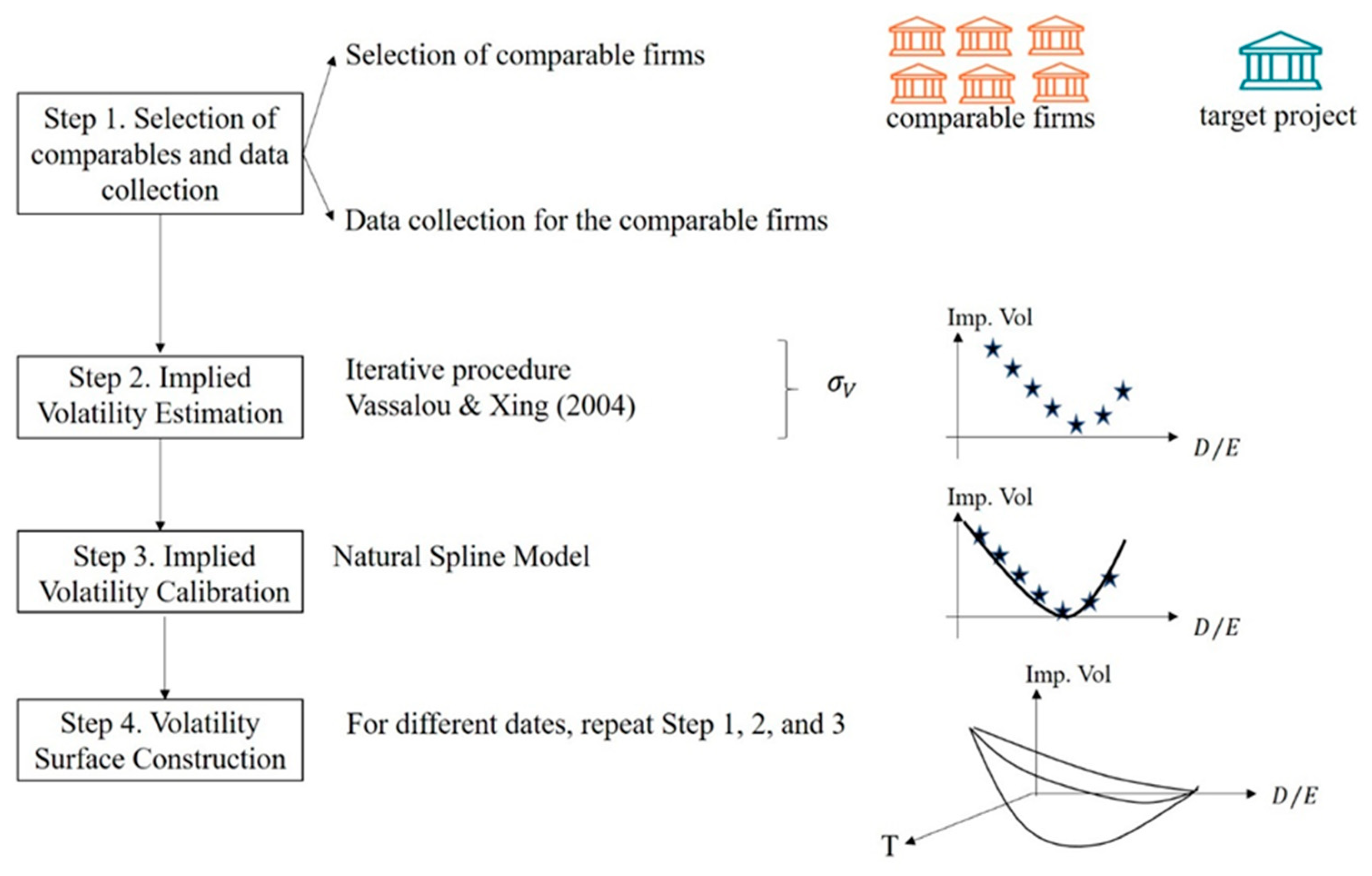
2. Materials and Methods
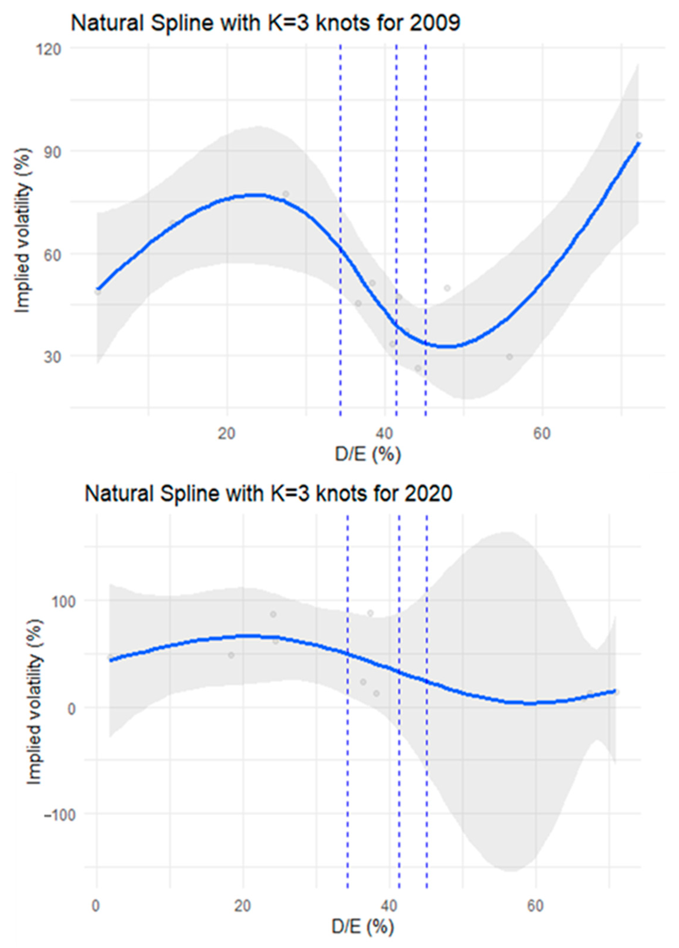
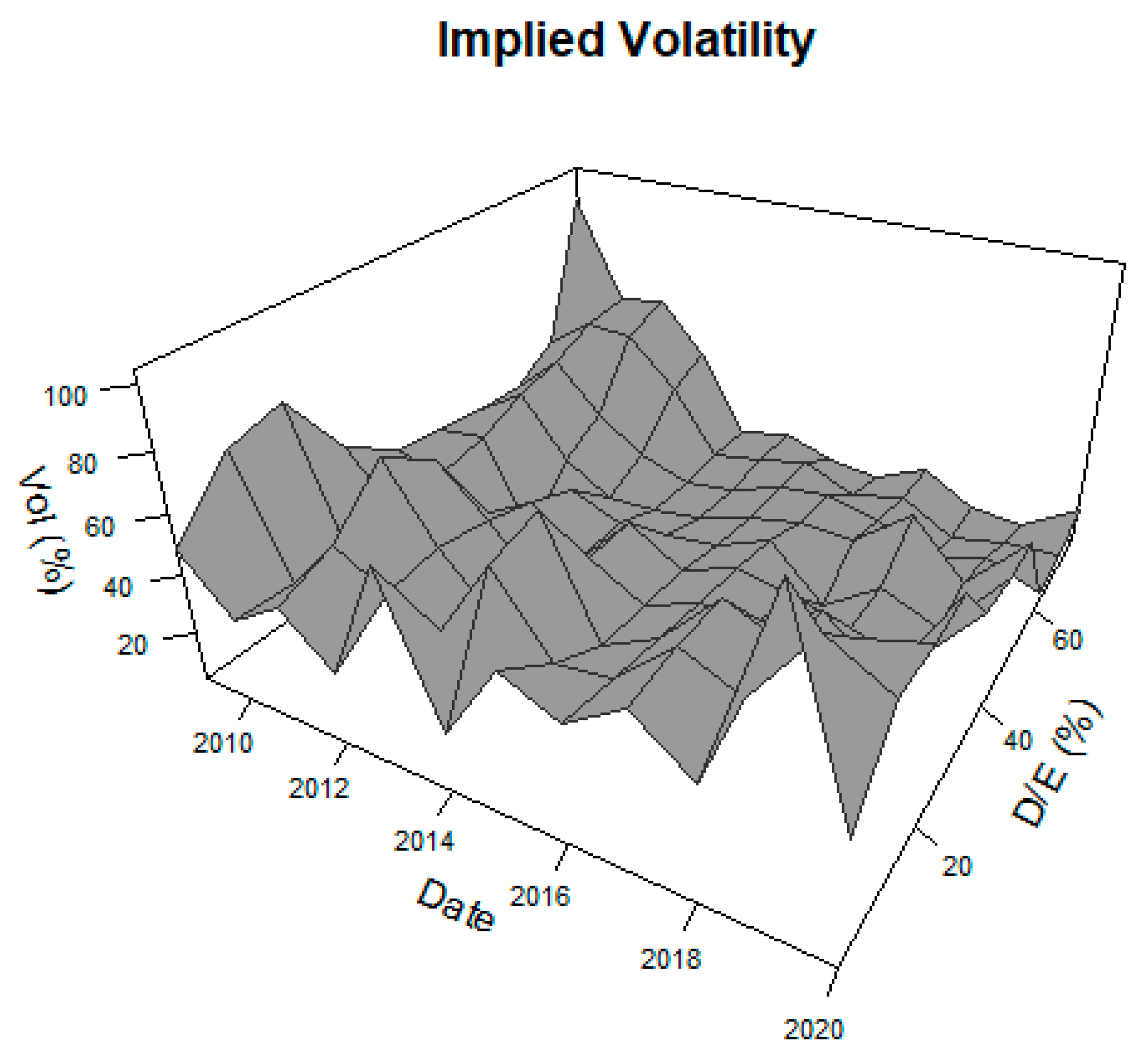
Merton’s model [16] has been successfully applied in structural models for credit risk frameworks, such as the KMV model, to estimate the distance-to-default (DD). To this end, different methodologies have been proposed to estimate necessary but unobservable variables such as the firm’s assets volatility and the face value of debt [22]. One of the first attempts was the proposal by Ronn and Verma [23] who developed two equations to solve these two unknowns. However, as noted by Milidonis and Stathopoulos [24], the disadvantage of this proposal is the non-consistency with Merton’s assumption of stochastic equity volatility. To overcome it, Duan [25] suggests a data transformation method based on the maximum likelihood, which seems to be superior to the previous methodology [24]. Moreover, several modifications have been introduced in the literature (see, e.g., [26] and the references therein; however, this method presents estimation problems when the likelihood function is relatively flat). An approach with similar results is the one proposed by Vassalou and Xing [27], which is an iterated procedure—as is the one utilized by the KMV model—to find the volatility and drift of the asset value. This method is considered an expectation–maximization (EM) algorithm, according to Duan et al. [28]. More recently, Christoffersen et al. [29] found that, although the maximum likelihood method yields similar results to the iterative approach for the usual levels of firm leverage, there are remarkable differences when asset values are comparatively lower than the face value of the firm’s debt. In addition, the authors argue that the KMV method cannot be seen as an EM algorithm, in contrast to Duan et al. [28], and consider the lognormality assumption as a salient drawback [26]. The iterative procedure, and similar methods, have been successfully employed in the literature in different applications. For instance, Lee [30] estimated the firm value and its volatility to assess the default probability in credit risk applications; this was followed by Charitou et al. [31], Doumpos et al. [32], Afik et al. [33], and more recently by Andreou et al. [34] and Levine and Wu [35]. Other similar approximations were applied by Zhang et al. [36] in the case of a bank’s liquidity risk framework and by Lovreta and Silaghi [37] to obtain the surface of CDS implied in a firm’s asset volatility.
Overall, Vassalou and Xing’s [27] methodology has major advantages for the estimation of asset volatility—see also [38]—and, based on this, we assume that the market value of the RE firm’s assets follows the GBM as expressed in Equation (1):
d V = μ V d t + σ V V d B
where V is the value of the assets of the renewable company, μ and σ V are the instantaneous drift and volatility, respectively, and B is a standard Brownian motion. According to the Black–Scholes–Merton formula, the equity’s market value ( E ) is given by:
E = V N d 1 D e r T t N d 2
where
d 1 = l n V / D + r + σ V 2 / 2 T σ V T
d 2 = d 1 σ V T
N d 1 and N d 2 represent the standard normal cumulative distribution functions, T is the time to maturity, and D is the market value of debt. Then, an iterative procedure is employed to solve the firm’s asset volatility, σ V . More details about the procedure are found in Christoffersen [39], and it is implemented in our work. In our study, we employ the 10-year treasury bill rate, which is equal to 1.5%, as the proxy for the risk-free rate (although the results are not sensitive to the use of other proxies), and the time to maturity is set to 2 years. An important input is the face value of debt, which is unobservable, and we assume that it is equal to the short-term debt plus one half of the long-term debt as per Vassalou and Xing [27], Bharath and Shumway [40], and Amaya et al. [41]. We also employ quarterly data of equity market value, and short- and long-term debt due to data availability. Data from the S&P/TSX RE and Clean Technology Index (This index measures performance of green technologies and sustainable infrastructure companies listed on the TSX. Constituents are screened by Sustainalytics. Source: us.spindices.com.) members were downloaded from Bloomberg. For the asset value, the current market capitalization (CUR_MKT_CAP ticker) proxy was employed, while for the short-term debt and the long-term debt variables, the BS_ST_BORROW and BS_LT_BORROW tickers, respectively, were utilized.
To estimate the implied volatilities, we employ the iterative method of BS_fit command included in the Distance to Default—‘DtD’ library of R—and the aforementioned variables.
Once the volatilities are estimated, these parameter values are calibrated by employing the natural spline model, which are b-spline in intermediate regions and linear splines in extremes. Specifically, natural spline models are a class of functions defined piecewise by the (cubic) polynomial, which is twice continuously differentiable, where the breakpoints (also called knots) divide disjoint segments in the data, and the regression function is fitted as a separate polynomial portion in each segment. For this reason, natural splines perform better than cubic splines in the tails. For more details, please see, e.g., Hastie ([42], Chapter 7).
We use the lm command from the ‘splines’ library of R, where the dependent variable is the estimated volatility in the previous step and the independent variables are their respective leverage ratios for each year. As usual, the selected knots are the first, second, and third quartiles. Figure 1 depicts an example for implied volatility estimations in 2009 and 2020.
Finally, after the implied volatilities are estimated and calibrated for each date of valuation, the volatility surface is obtained. For a given date, the graph of implied volatility against the debt-to-equity ratio can be represented and combined to obtain the surface shape. Hence, for a given date of valuation and the leverage ratio of a project, the (implied) volatility can be used to estimate the value of the project. It is noteworthy that we employ the date of the implied volatility estimation (namely, the valuation date) rather than the time to maturity used in the case of financial options. Although the main purpose of our work is to provide an adequate methodology to estimate volatility in order to valuate new RE projects, the implied volatility may also be used to valuate different strategic options, as can be seen in our empirical results. Figure 2 depicts our proposed methodology.

3. Results

For the sake of general application on RE projects, information about stocks from the S&P/TSX RE and Clean Technology Index is used to estimate the implied volatility in the period 2009–2020. From the 17 stocks listed in the index, 11 stocks (these companies are Brookfield Renewable Partners LP (Toronto, Canada), Ballard Power Systems Inc. (Burnaby, Canada), Boralex Inc. (Kingsey Falls, Canada), Cascades Inc. (Kingsey Falls, Canada), Clearwater Seafoods Inc. (Bedford, Canada), Innergex RE Inc. (Longueuil, Quebec, Canada), Northland Power Inc. (Toronto, Canada), SunOpta Inc. (Brampton, Canada), Village Farms International Inc. (Delta, Canada), 5N Plus Inc. (Montreal, Quebec, Canada), and Westport Fuel Systems Inc. (Vancouver, Canada)) were considered due to information availability. Table 1 shows the different renewable firms’ leverage ratios (Lev.) and their respective estimated volatility (Vol.) for each year following the iterated procedure proposed by Vassalou and Xing [27]. The data are sorted according to the leverage ratio, specifically, the debt-to-equity relationship.
As observed, the minimum volatility is 3.37% (when the debt-to-equity ratio is 62.7% in 2013) and the maximum is 113.38% (when the debt-to-equity proportion is 20.7% in 2019); however, the median of the estimated volatility ranges between 16.42% (2013) and 47.10% (2009). For RE data, the volatility surface at the annual basis is mapped in Figure 3. Different values of implied volatility are obtained based on the analyzed period and the leverage ratio of the sample.
To illustrate the utility of our methodology for the valuation of RE projects, this section presents three case studies.
  • Case Study 1
The first case is based on Eissa and Tian [43] who propose a novel methodology based on the construction of the Lobbato3C-Milstein (L3CM) method for real option valuation. In addition, the study applies the proposed L3CM methodology to value a solar power plant investment in the Arab Republic of Egypt, in particular to estimate the value of an option to delay. This real option value is estimated as the price of a European call option with the appropriate input variables. The details about the case study are found in [43] and are summarized in Table 2.
Based on selling electricity prices published in a local decree issued on July 2014 and using Abadie and Chamorro’s [44] methodology, the authors estimate a volatility of 10.45%. With this information, the option to delay is valued at $US 264.7410 by employing the BS formula for a European call option given in Equations (5)–(7):
C = S N d 1 I e r T N d 2
where
d 1 = l n V / D + r + σ V 2 / 2 T σ V T
d 2 = d 1 σ V T
Since the leverage ratio for this specific project is unknown, we employ the minimum and maximum implied volatility obtained from our methodology. In July 2014, these values correspond to 12.48% and 76.05%, respectively for RE projects. Thus, the range of the deferral option is between $US 264.748 and $US 297.363. Though the apparently significant differences between the employed volatilities, our result for the option valuation is similar to the one obtained by Eissa and Tian [43] and is mainly explained by the long time in which to invest.
  • Case Study 2
In this case study, we work with data sourced from Kroniger and Madlener [45]. The authors employ Monte Carlo simulations to obtain the main inputs to apply ROA to a hybrid wind power and hydrogen storage system. The details of the analysis for the project’s viability are found in their paper and we focus on the real option valuation for the base case. The impact of the hybrid energy system is also examined through real options in [46], especially the option to upgrade or reconfigure the system which affects the design choice. On the other hand, [47] employs real options to value wind power projects. Another valuation approach is the model proposed by McDonald and Siegel [48], where the value of the project, V, follows a GBM:
d V = α V d t + σ V d z
where α is the drift of the value process, σ is its volatility, and dz is the increment of a Brownian motion. We are interested in the value of the option to invest, given by:
F V = e r T m a x E V T I
where r is the discount rate, T is the time that the investment is performed, E is the expected value operator, and I is the cost of the investment, which is assumed to be known and fixed. Departing from the Bellman equation:
r F d t = E d F
and applying Itô’s lemma to dF, it is shown that:
1 2 σ 2 V 2 F V + α V F V r F = 0
Thus F V must satisfy the following boundary conditions:
F 0 = 0
F V * = V * I
F V * = 1
where V *   is a critical value such that it is optimal to invest when V V * . The first condition means that the option to invest has no value if V = 0 , whereas the second condition is the value-matching condition and the third condition is the so-called smooth-pasting condition. A typical solution, which satisfies the first boundary condition, for the differential equation is in the form of:
F V = A V β 1
where A is a constant and β 1 > 1 . The second and third boundary conditions are employed to find A and V * , and thus:
A = β 1 1 β 1 1 β 1 β 1 I β 1 1
V * = β 1 β 1 1 I
Finally, the value of β 1 that satisfies the condition ( β 1 > 1 ) is:
β 1 = 1 2 r σ 2 + r σ 2 1 2 2 + r σ 2 .
In the application, the authors set α = 0 and I = 1 for simplicity, and the discount rate is 4%. For more details about the derivation of the model, see, e.g., Dixit and Pindyck [5]. As an alternative for the project volatility, we employ the closest date (Jan 2014) for the lowest and highest volatility estimated using our procedure for RE projects. The results are presented in Table 3.
The volatility used by Kroniger and Madlener [45] is between the lowest and highest implied volatility of our work (12.48–76.05%), but close to the estimated median of the implied volatility (20.19%).
  • Case Study 3
Torani et al. [49] examine the adoption of solar photovoltaic energy by employing a stochastic dynamic model. In the same line as with the previous case, the authors extend the Bellman equation to consider two variables, which are the long-term price of electricity ( P ) and the cost of solar ( C ) . The dynamics for each of these variables are given by:
d P = α P P d t + σ P P d z P
d C = α C C d t + σ C C d z C
where α P ( α C ) is the drift of the electricity price (cost of solar) process, σ P and σ C are the volatilities of the respective processes, and d z P and d z C are the increments of a Wiener process or Brownian motion. Thus, the Bellman equation considering the two variables is:
1 2 σ P 2 P 2 F P P + 2 γ σ P σ C P C F P C + σ C 2 C 2 F C C + α P P F P + α C C F C r F = 0
where γ is the correlation between P and C . The solution for F is analogous to the previous case (one variable), and β 1 is given by
β 1 = 1 2 α P α C σ 2 + α P α C σ 2 1 2 2 + 2 r α C σ 2
and
σ 2 = σ P 2 2 γ σ P σ C + σ C 2
Interestingly, the authors find that:
P R O A * = β 1 β 1 1 P N P V *
where P N P V * and P R O A * are the threshold electricity price at which a residential or commercial consumer will adopt solar photovoltaic energy according to the N P V and   R O A rules, respectively. Once again, we are interested in the valuation result and more details are found in Torani et al. [49]. Table 4 presents the comparison of the results obtained by using the volatility extracted from the volatility surface for real options and r = 3% discount rate.
The authors employ σ P = σ C = 0.1409 and γ = 0 ; therefore, their volatility estimation is 20.07% according to Equation (23). We also assume that the drift values are α P = 0.0289 and α C = −0.0441, and P N P V * as per the study by Torani et al.; however, for the project’s volatility, we apply our proposal, which yields a more appropriate volatility estimation for this RE case study. Since there is no information about the leverage ratio of the project, we employ the information provided in Table 1, with a mean (median) implied volatility of 22.69% (16.42%). Otherwise, we could extract the implied volatility corresponding to the debt-to-equity relation in 2013 from the volatility surface. Thus, replacing the values for σ , α P , and α C in Equation (22) we obtain a value of 1.0111 and 1.027 for β 1 as can be seen in columns 2 and 3 of Table 4. Finally, we apply Equation (24) to find the threshold electricity price at which a residential or commercial consumer will adopt solar photovoltaic energy according to ROA.

4. Discussion

The empirical results demonstrate that the implied volatility ranged from 3.37% to 113.78% in the period from January 2014 to December 2020 for the RE projects. This difference is explained by the dissimilar leverage ratios employed by the analyzed companies. Despite the relatively high range found in the estimated implied volatility, its median for different years ranged between 16.42% and 47.10%. As a matter of fact, these estimates have an impact on the valuation of real options, which would be relevant for practitioners and managers, particularly those deciding on undertaking RE projects. Furthermore, the lower implied volatility of renewable companies (compared with oil companies) supports investment in renewable projects and contributes to a more efficient transition to renewable and cleaner energy.
In an environment where the urgent implementation of renewable energy projects is paramount, the incorporation of real options valuation methodologies allows for a broader evaluation of the viability of these projects that would surely be discarded under traditional methodologies. In particular, the characteristics of solar photovoltaic projects provide an extreme validation of the usefulness of the real option valuation methodology. First, given a fixed and inelastic energy demand, the supply of solar energy is inflexible, since its availability is limited by the effective hours of sunshine. Consequently, the interaction of supply and demand for solar energy can lead to negative energy prices in the market at certain time points, which implies higher price volatility for any investment project feasibility assessment. Second, because of the potential existence of negative prices, traditional project evaluation methodologies would not provide an opportunity for project development. However, the real options methodology allows for the value in waiting or delaying for a better moment for a project’s development to be quantified, based on changes in energy demand patterns or on the appearance of new energy storage technologies that allow for a better cost-efficiency ratio for this type of energy generation. Finally, the valuation of the best moment to implement this type of project is especially valuable in a technology such as solar, which is quicker to implement, e.g., some months compared to years for other renewal energy options such as hydroelectric power plants, wind power and geothermal. To the extent that real options valuation maintains solar photovoltaic projects as active instead of being discarded, changes in the demand or supply situation can be capitalized in a short period of time.

5. Conclusions

RE project valuation requires accurate tools to estimate volatility, a problem that has not been satisfactorily addressed in the literature. We cover this remarkable gap by suggesting a method to estimate volatility for new and RE projects that follows the ROA and thus is based on the concept of implied volatility for financial options. This method is also applicable to conventional energy projects, such as the oil-based projects, which have been extensively studied in the literature, and other types of projects for which market data are available.
As the framework is based on the concept of implied volatility for financial options, we employed the debt-to-equity ratio for real options instead of the moneyness or strike price used in the case of financial options. To this end, we applied the natural spline model to calibrate the implied volatilities. We described our proposal in a step-by-step procedure to be implemented for RE project valuation, which allows for flexibility in managerial decisions. To the best of our knowledge, this is the first study to implement the volatility surface for renewable and conventional energy projects. The main advantages of the implied volatility model (for financial options) are its ability to provide more accurate results and its widespread acceptance among academics and practitioners. Furthermore, we consider that this is a natural and straightforward way to estimate the volatility for ROA, since real option valuation is derived from the same ideas and tools as those used for financial options.
Future research should also be focused on forecasting the implied volatility of energy projects using the techniques proposed in this paper, given the importance of such predictions on decision making, e.g., extreme volatility in oil prices resulting in a decline in manufacturing activity [50] and other types of projects for which market data are available. Thus, a forecast of implied volatility may also help to anticipate real effects on the economy and aid in decision-making processes that incentivize managers to not delay or abandon valuable projects. A new strand in the literature is also pointing towards the analysis of (renewable) energy portfolios [51,52,53]; accordingly, our methodology can be extended to consider investments in projects based on portfolios. Finally, another avenue for research is the use of the Lévy and geometric Lévy process for the calibration of RE projects and a comparison of the results with our methodology.

Author Contributions

R.-I.G.-M.: Methodology, Reviewing and Editing. J.M.-M.: Conceptualization, Software, Writing. A.M.-V.: Conceptualization, Methodology, Software, Writing. J.P.: Conceptualization, Writing, Reviewing and Editing. All authors have read and agreed to the published version of the manuscript.

Funding

This work was supported by the University of Salamanca under Research Program I.A 2022; Universidad del Rosario, School of Management; the Gabriel Vegalara educational fund; the Colombian Department of Science, Technology and Innovation [COLCIENCIAS-757 call] and the FAPA-Uniandes, Colombia [PR.3.2016.2807].

Data Availability Statement

The data presented in this study are available on request from the corresponding author. The data are not publicly available due to Bloomberg property rights.

Acknowledgments

Authors acknowledge the comments received by participants in the CEM 2018, EFMA 2018 and the ICASQF 2019 conferences which significantly enhanced the quality and rigor of this study.

Conflicts of Interest

The authors declare no conflicts of interest.

References

  1. Liu, Y.; Zheng, R.; Chen, S.; Yuan, J. The economy of wind-integrated-energy-storage projects in China’s upcoming power market: A real options approach. Resour. Policy 2019, 63, 101434. [Google Scholar] [CrossRef]
  2. Aquila, G.; de Queiroz, A.R.; Balestrassi, P.P.; Junior, P.R.; Rocha, L.C.S.; Pamplona, E.O.; Nakamura, W.T. Wind energy investments facing uncertainties in the Brazilian electricity spot market: A real options approach. Sustain. Energy Technol. Assess 2020, 42, 100876. [Google Scholar] [CrossRef]
  3. Gupta, S.D. Using real options to value capacity additions and investment expenditures in renewable energies in India. Energy Policy 2021, 148, 111916. [Google Scholar] [CrossRef]
  4. Li, L.; Cao, X. Comprehensive effectiveness assessment of energy storage incentive mechanisms for PV-ESS projects based on compound real options. Energy 2020, 239, 121902. [Google Scholar] [CrossRef]
  5. Dixit, R.K.; Pindyck, R.S. Investment under Uncertainty; Princeton University Press: Princeton, NJ, USA, 1994. [Google Scholar]
  6. Cui, X.; Shibata, T. Investment strategies, reversibility, and asymmetric information. Eur. J. Oper. Res. 2017, 263, 1109–1122. [Google Scholar] [CrossRef]
  7. Li, Y.; Wu, M.; Li, Z. A real options analysis for RE investment decisions under China carbon trading market. Energies 2018, 11, 1817. [Google Scholar] [CrossRef]
  8. Smith, J.E. Alternative Approaches for Solving Real-Options Problems: (Comment on Brandão et al. 2005). Decis. Anal. 2005, 2, 89–102. [Google Scholar] [CrossRef]
  9. Godinho, P. Monte Carlo estimation of project volatility for real options analysis. J. Appl. Financ. 2006, 16, 15–30. [Google Scholar]
  10. Brandão, L.E.; Dyer, J.S.; Hahn, W.J. Volatility estimation for stochastic project value models. Eur. J. Oper. Res. 2012, 220, 642–648. [Google Scholar] [CrossRef]
  11. Ritzenhofen, I.; Spinler, S. Optimal design of feed-in-tariffs to stimulate RE investments under regulatory uncertainty—A real options analysis. Energy Econ. 2016, 53, 76–89. [Google Scholar] [CrossRef]
  12. Zhang, M.M.; Zhou, D.Q.; Zhou, P.; Chen, H.T. Optimal design of subsidy to stimulate RE investments: The case of China. Renew. Sust. Energ. Rev. 2017, 71, 873–883. [Google Scholar] [CrossRef]
  13. Lima, G.A.C.; Suslick, S.B. Estimating the volatility of mining projects considering price and operating cost uncertainties. Resour. Policy 2006, 31, 86–94. [Google Scholar] [CrossRef]
  14. Brach, M.A.; Paxson, D.A. A gene to drug venture: Poisson options analysis. R&D Manag. 2001, 31, 203–214. [Google Scholar]
  15. Mun, J. Real Options Analysis–Tools and Techniques for Valuing Strategic Investments and Decisions; John Wiley& Sons. Inc.: Hoboken, NJ, USA, 2002. [Google Scholar]
  16. Merton, R.C. On the pricing of corporate debt: The risk structure of interest rates. J. Financ. 1974, 29, 449–470. [Google Scholar]
  17. Lewis, N.A.; Eschenbach, T.G.; Hartman, J.C. Can we capture the value of option volatility? Eng. Econ. 2008, 53, 230–258. [Google Scholar] [CrossRef]
  18. Nicholls, G.M.; Lewis, N.A.; Zhang, L.; Jiang, Z. Breakeven volatility for real option valuation. Eng. Manag. J. 2014, 26, 49–61. [Google Scholar] [CrossRef]
  19. Godinho, P. Simulation-based estimation of state-dependent project volatility. Eng. Econ. 2018, 63, 188–216. [Google Scholar] [CrossRef]
  20. Myers, S.C.; Read, J.A. Real Options, Taxes and Financial Leverage (No. w18148); National Bureau of Economic Research: Cambridge, MA, USA, 2012. [Google Scholar] [CrossRef]
  21. Myers, S.C.; Read, J.A. Real Options and Hidden Leverage. J. Appl. Corp. Financ. 2022, 34, 67–80. [Google Scholar] [CrossRef]
  22. Byström, H. An alternative way of estimating asset values and asset value correlations. J. Fixed Income 2011, 21, 30–38. [Google Scholar] [CrossRef]
  23. Ronn, E.I.; Verma, A.K. Pricing risk-adjusted deposit insurance: An option-based model. J. Financ. 1986, 41, 871–895. [Google Scholar]
  24. Milidonis, A.; Stathopoulos, K. Do US insurance firms offer the “wrong” incentives to their executives? J. Risk Insur. 2011, 78, 643–672. [Google Scholar] [CrossRef]
  25. Duan, J.C. Maximum likelihood estimation using price data of the derivative contract. Math. Financ. 1994, 4, 155–167, Erratum in Math. Financ. 2000, 10, 461–462. [Google Scholar] [CrossRef]
  26. Ben-Abdellatif, M.; Ben-Ameur, H.; Chérif, R.; Fakhfakh, T. Quasi-maximum likelihood for estimating structural models. Les Cahiers GERAD ISSN 2021, 711, 2440. [Google Scholar]
  27. Vassalou, M.; Xing, Y. Default risk in equity returns. J. Financ. 2004, 59, 831–868. [Google Scholar] [CrossRef]
  28. Duan, J.C.; Gauthier, G.; Simonato, J.G. On the Equivalence of the KMV and Maximum Likelihood Methods for Structural Credit Risk Models; Groupe D’études et de Recherche en Analyse des Décisions: Montréal, QC, Canada, 2005. [Google Scholar]
  29. Christoffersen, B.; Lando, D.; Nielsen, S.F. Estimating volatility in the Merton model: The KMV estimate is not maximum likelihood. Math. Financ. 2022, 32, 1214–1230. [Google Scholar] [CrossRef]
  30. Lee, W.C. Redefinition of the KMV model’s optimal default point based on genetic-algorithms–Evidence from Taiwan. Expert Syst. Appl. 2011, 38, 10107–10113. [Google Scholar] [CrossRef]
  31. Charitou, A.; Dionysiou, D.; Lambertides, N.; Trigeorgis, L. Alternative bankruptcy rediction models using option-pricing theory. J. Bank Financ. 2013, 37, 2329–2341. [Google Scholar] [CrossRef]
  32. Doumpos, M.; Niklis, D.; Zopounidis, C.; Andriosopoulos, K. Combining accounting data and a structural model for predicting credit ratings: Empirical evidence from european listed firms. J. Bank Financ. 2015, 50, 599–607. [Google Scholar] [CrossRef]
  33. Afik, Z.; Arad, O.; Galil, K. Using Merton model for default prediction: An empirical assessment of selected alternatives. J. Empir. Financ. 2016, 35, 43–67. [Google Scholar] [CrossRef]
  34. Andreou, C.K.; Lambertides, N.; Panayides, P.M. Distress risk anomaly and misvaluation. Br. Account. Rev. 2021, 53, 100972. [Google Scholar] [CrossRef]
  35. Levine, O.; Wu, Y. Asset Volatility and Capital Structure: Evidence from Corporate Mergers. Manag. Sci. 2021, 67, 2773–2798. [Google Scholar] [CrossRef]
  36. Zhang, J.; He, L.; An, Y. Measuring banks’ liquidity risk: An option-pricing approach. J. Bank Financ. 2020, 111, 105703. [Google Scholar] [CrossRef]
  37. Lovreta, L.; Silaghi, F. The surface of implied firm’s asset volatility. J. Bank Financ. 2020, 112, 105253. [Google Scholar] [CrossRef]
  38. Forssbæck, J.; Vilhelmsson, A. Predicting Default–Merton vs. Leland. Leland. 2017. Available online: https://papers.ssrn.com/sol3/papers.cfm?abstract_id=2914545 (accessed on 9 February 2017).
  39. Christoffersen, B. Distance to Default Package. 2020. Available online: https://cran.r-project.org/web/packages/DtD/vignettes/Distance-to-default.pdf (accessed on 19 March 2023).
  40. Bharath, S.T.; Shumway, T. Forecasting default with the Merton distance to default model. Rev. Financ. Stud. 2008, 21, 1339–1369. [Google Scholar] [CrossRef]
  41. Amaya, D.; Boudreault, M.; McLeish, D.L. Maximum likelihood estimation of first-passage structural credit risk models correcting for the survivorship bias. J. Econ. Dyn. Control 2019, 100, 297–313. [Google Scholar] [CrossRef]
  42. Hastie, T.J. Generalized additive models. In Statistical Models in S; Chambers, J.M., Hastie, T.J., Eds.; Wadsworth & Brooks/Cole: Pacific Grove, CA, USA, 1992. [Google Scholar]
  43. Eissa, M.A.; Tian, B. Lobatto-Milstein Numerical Method in Application of Uncertainty Investment of Solar Power Projects. Energies 2017, 10, 43. [Google Scholar] [CrossRef]
  44. Abadie, L.M.; Chamorro, J.M. Valuation of real options in crude oil production. Energies 2017, 10, 1218. [Google Scholar] [CrossRef]
  45. Kroniger, D.; Madlener, R. Hydrogen storage for wind parks: A real options evaluation for an optimal investment in more flexibility. Appl. Energy 2014, 136, 931–946. [Google Scholar] [CrossRef]
  46. Binder, W.R.; Paredis, C.J.J.; Garcia, H.E. The Value of Flexibility in the Design of Hybrid Energy Systems: A Real Options Analysis. IEEE Power Energy Technol. Syst. J. 2017, 4, 74–83. [Google Scholar] [CrossRef]
  47. Martinez-Cesena, E.A.; Mutale, J. Wind Power Projects Planning Considering Real Options for the Wind Resource Assessment. IEEE Trans. Sustain. Energy 2012, 3, 158–166. [Google Scholar]
  48. McDonald, R.; Siegel, D. The value of waiting to invest. Quart. J. Econ. 1986, 101, 707–727. [Google Scholar] [CrossRef]
  49. Torani, K.; Rausser, G.; Zilberman, D. Innovation subsidies versus consumer subsidies: A real options analysis of solar energy. Energy Policy 2016, 92, 255–269. [Google Scholar] [CrossRef]
  50. Elder, J.; Serletis, A. Volatility in Oil Prices and Manufacturing Activity: An Investigation of Real Options. Macroecon Dyn. 2011, 15 (Suppl. 3), 379–395. [Google Scholar] [CrossRef]
  51. Passos, A.C.; Street, A.; Barroso, L.A. A Dynamic Real Option-Based Investment Model for Renewable Energy Portfolios. IEEE Trans. Power Syst. 2017, 32, 883–895. [Google Scholar] [CrossRef]
  52. Ghamkhari, M.; Wierman, A.; Mohsenian-Rad, H. Energy Portfolio Optimization of Data Centers. IEEE Trans. Smart Grid 2017, 8, 1898–1910. [Google Scholar] [CrossRef]
  53. Belz, A.; Giga, A. Of Mice or Men: Management of Federally Funded Innovation Portfolios with Real Options Analysis. IEEE Eng. Manag. Rev. 2018, 46, 1–35. [Google Scholar] [CrossRef]
Figure 1. Natural spline fitted to the implied volatility data for 2009 (upper panel) and 2020 (bottom panel) with k = 3 knots. Vertical lines represent the first, second, and third quartiles. Grey areas correspond to 95% confidence intervals. The graphs were obtained using the ‘splines’ library of R.
Energies 17 01225 g001
Figure 2. Procedure of estimation for the project volatility surface [27]. Stars correspond to the implied volatility estimates following the iterative procedure.
Energies 17 01225 g002
Figure 3. Volatility surface for RE data (annual basis). The graph originated from R 4.2.2 using the library plot3D and the proposed methodology.
Energies 17 01225 g003
Table 1. Implied volatility estimation for the analyzed renewable companies.
2009MeanMedian
Lev (%)3.5513.0127.3336.5640.9342.7144.1947.9155.7972.2338.4241.82MinMax
Vol (%)48.7968.7577.4545.4133.4837.2726.3749.8529.8894.5851.1847.1026.3794.58
2010MeanMedian
Lev (%)3.4810.5923.0829.3636.0040.1546.2549.4458.9863.1536.0538.07MinMax
Vol (%)30.5230.9329.4127.1836.7529.8545.2357.1331.4268.6238.7031.1827.1868.62
2011MeanMedian
Lev (%)24.1525.6531.0935.1440.1647.0253.3255.5261.9963.7043.7743.59MinMax
Vol (%)52.7732.0187.4136.7528.065.658.4247.3828.0275.7340.2234.385.6587.41
2012MeanMedian
Lev (%)16.4726.7636.1538.5242.1044.8951.3357.0660.8661.7843.5943.49MinMax
Vol (%)35.2120.0735.4281.9016.2118.917.1132.588.4357.4131.3326.337.1181.90
2013MeanMedian
Lev (%)13.4322.7927.0438.9639.2742.6859.7559.9962.0762.7342.8740.98MinMax
Vol (%)69.6333.4921.176.2040.159.9213.0210.1519.813.3722.6916.423.3769.63
2014MeanMedian
Lev (%)12.9622.8424.7538.4738.6844.7057.4158.7963.5071.5043.3641.69MinMax
Vol (%)21.7576.0551.6543.0637.3615.7712.4818.6312.6115.1030.4520.1912.4876.05
2015MeanMedian
Lev (%)19.1329.2237.5737.6239.6046.2863.6463.8365.3573.8147.6142.94MinMax
Vol (%)47.7649.7417.709.0845.7321.7421.0724.8112.249.6625.9521.419.0849.74
2016MeanMedian
Lev (%)19.8530.3533.5936.7138.3041.8059.8061.9971.7074.9546.9140.05MinMax
Vol (%)40.3554.4227.0113.0056.9627.1127.8820.469.028.6728.4927.068.6756.96
2017MeanMedian
Lev (%)20.0223.4227.1436.3938.0747.0561.3870.7871.9077.5547.3742.56MinMax
Vol (%)32.0785.4468.9823.887.1434.3922.1617.936.725.3330.4023.025.3385.44
2018MeanMedian
Lev (%)20.5626.7628.2531.4338.2456.7863.7171.6072.2772.3248.1947.51MinMax
Vol (%)26.7083.3063.3512.8920.6040.6626.004.6110.067.8529.6023.304.6183.30
2019MeanMedian
Lev (%)20.7526.6830.2437.4540.8359.2161.3668.8571.8773.6949.0950.02MinMax
Vol (%)113.3835.74101.6820.1815.0033.0010.699.665.439.1135.3917.595.43113.38
2020MeanMedian
Lev (%)1.8318.2824.1224.4736.3737.3738.1266.5767.3770.9838.5536.87MinMax
Vol (%)46.0348.7186.3361.2722.8187.2313.058.2313.1313.6740.0534.428.2387.23
Table 2. Parameters employed for option valuation in Case Study 1.
ParameterSymbolValueUnit
Current cash flow from investmentS302.8878$US million
Fixed investment costI340$US million
Time to investT25Years
Volatility σ 0.1045
Risk-free discount rater0.0875
Source: Eissa and Tian [43].
Table 3. Results comparison on option valuation of Case Study 2.
Kroniger and Madlener [45]Lowest Vol
(January 2014)
Highest Vol
(January 2014)
σ 0.21000.12480.7605
β 1 1.93672.82091.1232
A 0.26150.15980.6782
V * 2.06761.54929.1199
F V * 1.06760.54928.1199
Table 4. Results comparison on option valuation of the case study.
Calculations Based on Torani et al. [49] Mean Vol in 2013 (Our Study)Median Vol in 2013 (Our Study)
σ 0.20070.22690.1642
α P 0.02890.02890.0289
α C −0.0441−0.0441−0.0441
β 1 1.01181.01111.0127
P N P V * 0.01020.01020.0102
P R O A * 0.87600.92850.8137
Disclaimer/Publisher’s Note: The statements, opinions and data contained in all publications are solely those of the individual author(s) and contributor(s) and not of MDPI and/or the editor(s). MDPI and/or the editor(s) disclaim responsibility for any injury to people or property resulting from any ideas, methods, instructions or products referred to in the content.

