

Revolutionizing Wind Power Prediction—The Future of Energy Forecasting with Advanced Deep Learning and Strategic Feature Engineering

Abstract
:1. Introduction
- Extensive analysis of multiple single and hybrid decomposition methods and their combinations is performed to efficiently break down the wind generation data, resulting in important insights into seasonal and internal patterns.
- By using a feature selection approach to optimize the model inputs, we ensure that only highly correlated features are incorporated into the forecasting model.
- Proficient adjustment of hyperparameters refines the performance and precision of the forecasting model.
- A comprehensive comparison with cutting-edge deep learning models is carried out to verify the superiority of the proposed model in predicting wind energy power generation.
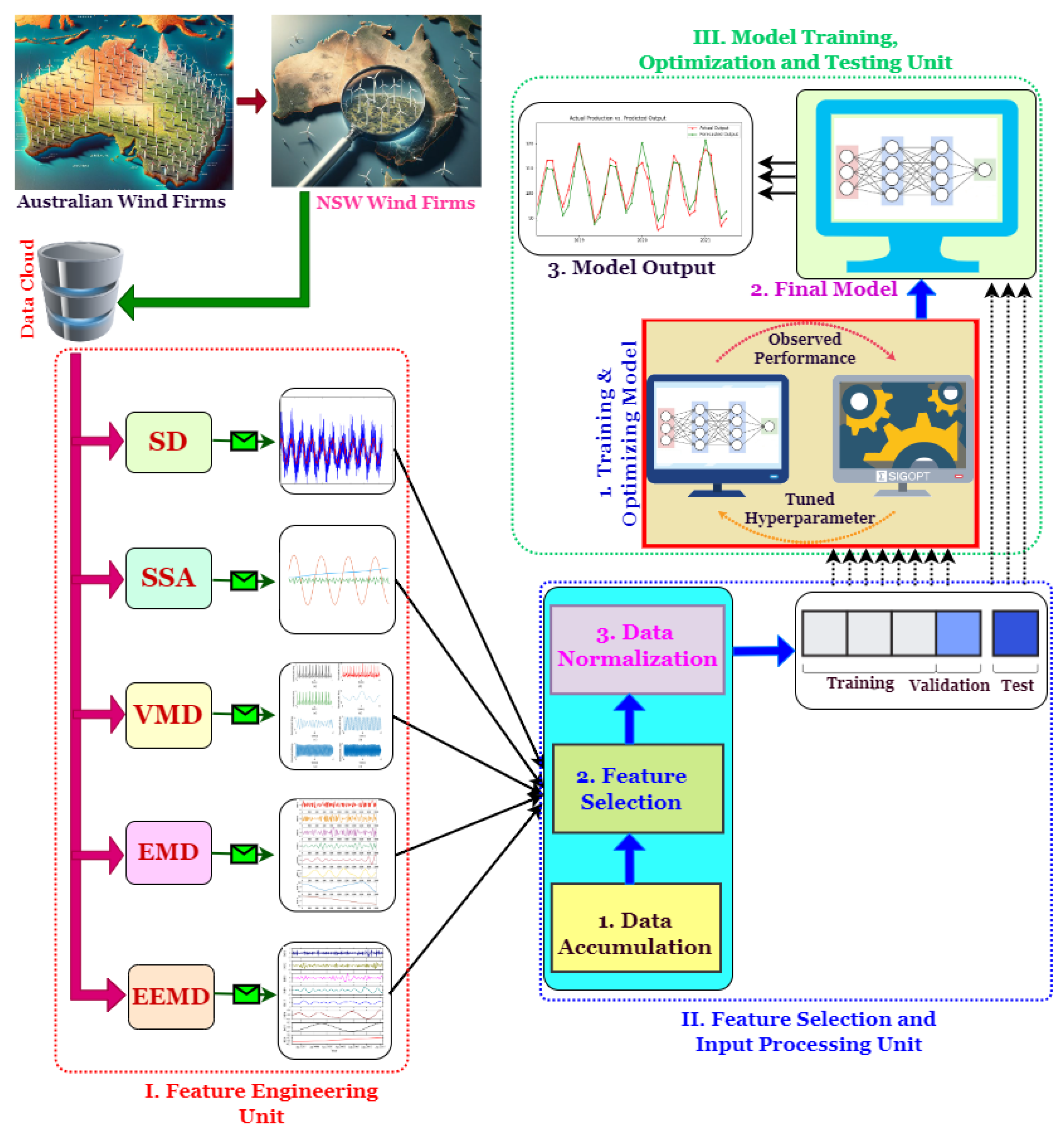
2. Methodology and Model Description
2.1. Feature Engineering Unit
2.1.1. Seasonal Decomposition (SD)
2.1.2. Singular Spectrum Analysis (SSA)
2.1.3. Variational Mode Decomposition (VMD)
2.1.4. Emperical Mode Decomposition (EMD)
- Identify the extrema (local maxima and minima) in the signal.
- Create upper and lower envelopes by connecting the extrema.
- Calculate the mean of the envelopes as a function of time.
- Subtract the mean from the original signal to obtain the first IMF.
- Iteratively sift the IMF to refine it.
- Extract subsequent IMFs from the residue.
- Repeat the process until no further IMFs can be found.
- Let us assume that a given signal is decomposed sequentially into its constituent IMFs. First, local maxima and minima are identified to form upper and lower envelopes. These envelopes are averaged to obtain the local mean . The residual is calculated by subtracting from the cumulative total of previous proto-IMFs, as shown in Equation (17). Equation (18) demonstrates the process of subtracting from to obtain , which is used for the next iteration. For the first iteration,The second iteration uses the updated signal from the previous iteration as the input signal. The upper and lower envelopes are updated as a result of recalculating the local maxima and minima. In Equation (19), the residual is calculated using and for this iteration. The derivation of from for the following iteration is shown in Equation (20).This iterative improvement process is continued until the n-th iteration. Equations (21) and (22) respectively yield the residual and cumulative sum produced in the same way. This iterative modification continues until the residual converges to zero, which indicates that the proto-IMF is complete and meets the IMF criteria. Convergence is indicated by the limit as n approaches infinity ().The first step in determining the IMF is to compute each proto-IMF using the set of equations in Equation (25). To obtain the final IMF (), the proto-IMFs are added together to form a single function that represents the inherent oscillatory mode of the original signal .
2.1.5. Ensemble Empirical Mode Decomposition (EEMD)
- Introduce a white noise seriesto the original power series, where represents the original time series data and is the white noise series, then determine the EMD related components.
- Determine the local maxima and minima of .
- Construct the upper envelope and lower envelope .
- Repeat Steps 1–3 until is less than or equal to a preset threshold indicating the allowable error by substituting for . Assigning as the initial EMD component of , the residual is
- The time series y(t) can be expressed as a sum of its IMFs and a residue, as follows:where denotes the IMFs and is the final residue.
2.2. Feature Selection and Input Processing Unit
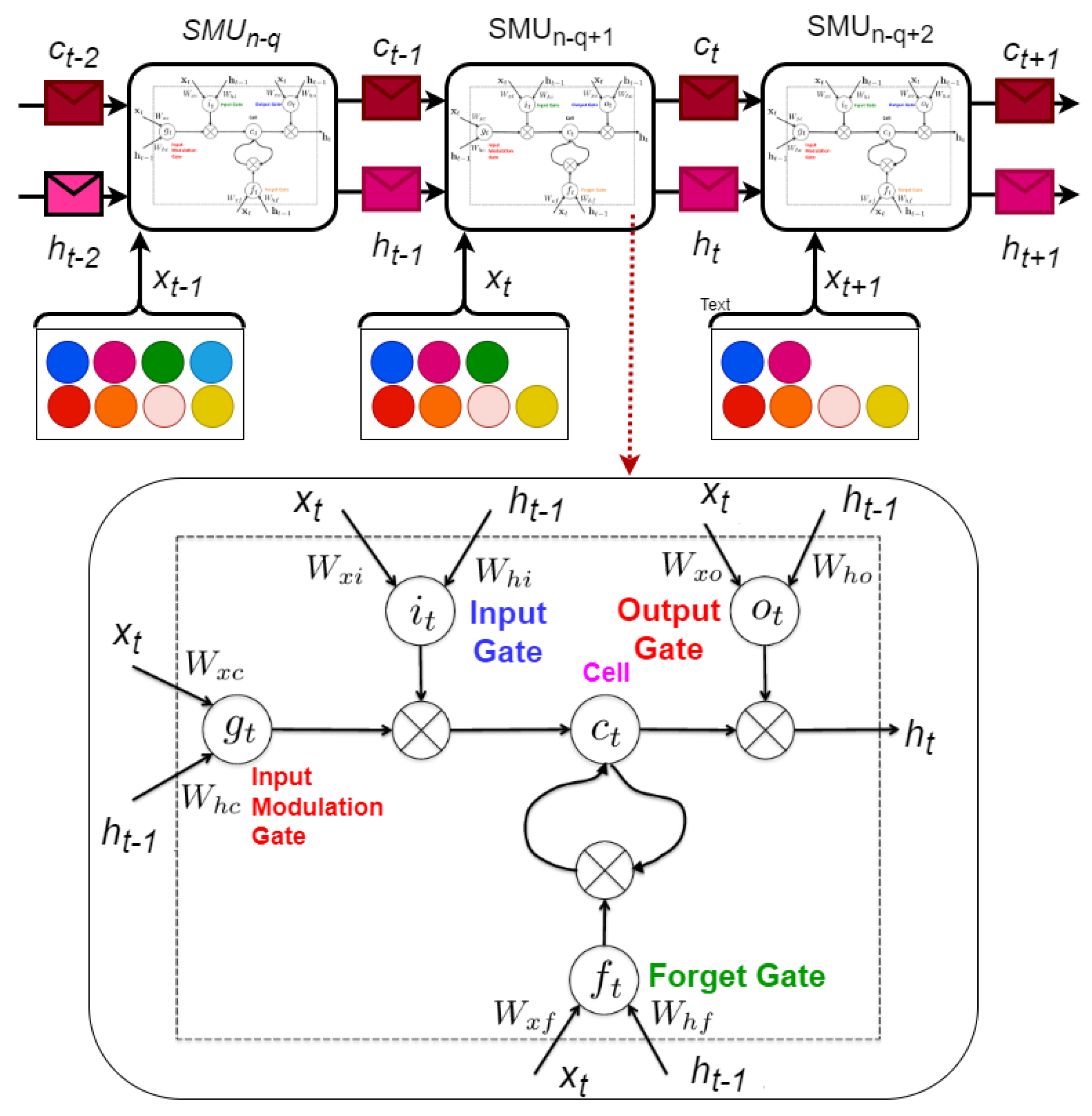
2.3. Model Training, Optimization, and Testing Unit
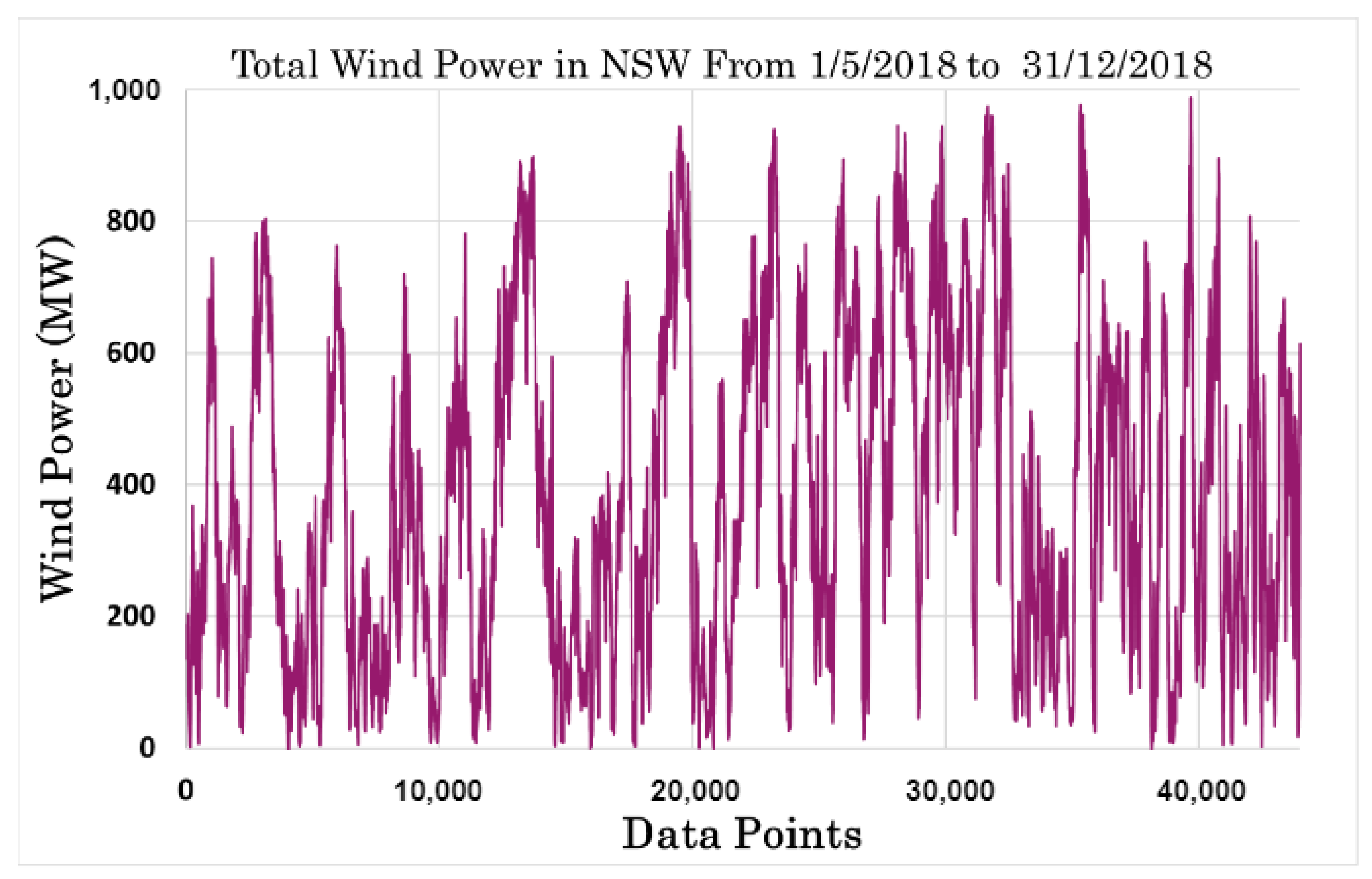
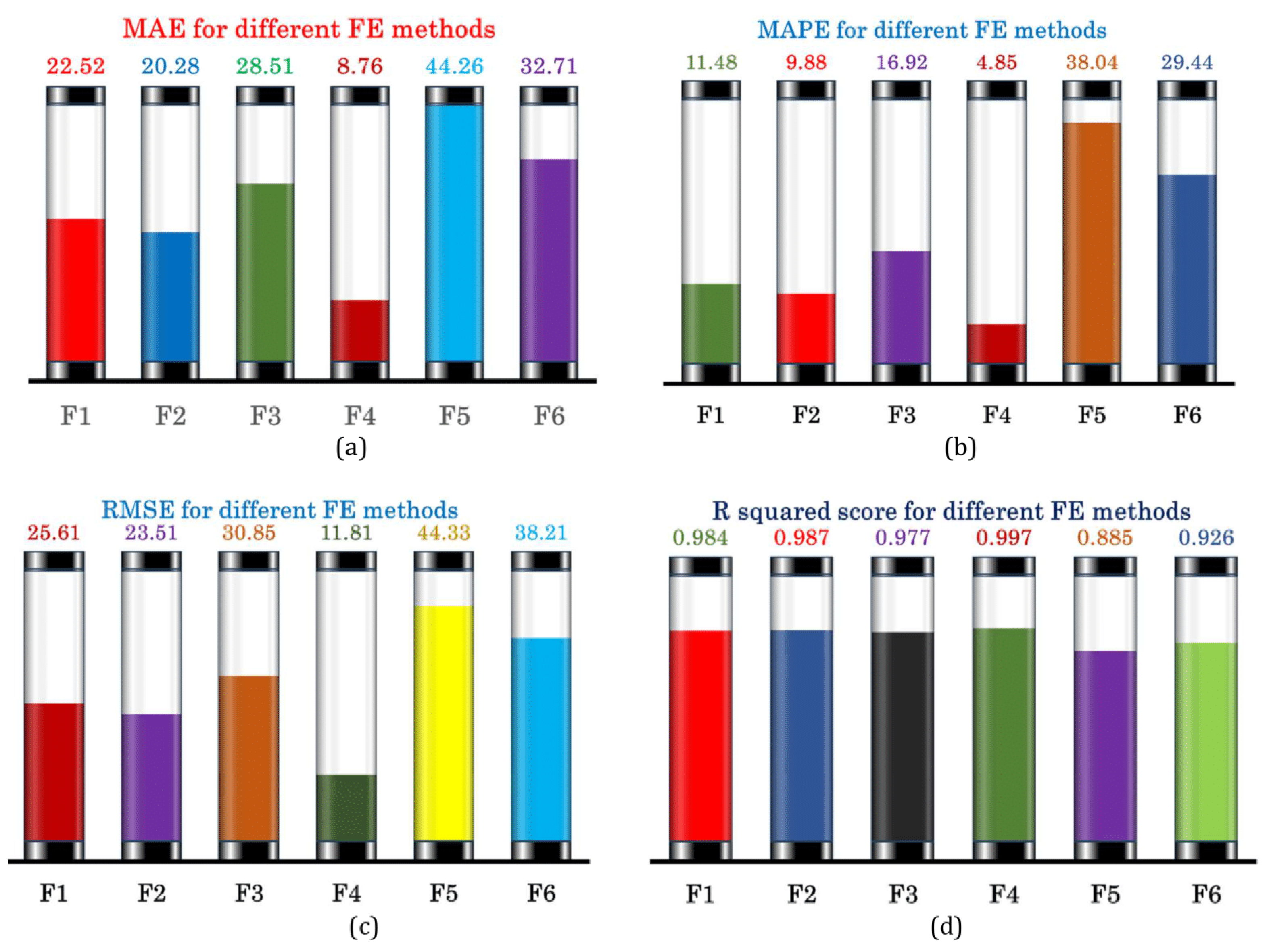
3. Results and Discussion
4. Conclusions and Future Directions
Author Contributions
Funding
Data Availability Statement
Conflicts of Interest
References
- Swain, R.B.; Karimu, A. Renewable electricity and sustainable development goals in the EU. World Dev. 2020, 125, 104693. [Google Scholar] [CrossRef]
- Cantarero, M.M.V. Of renewable energy, energy democracy, and sustainable development: A roadmap to accelerate the energy transition in developing countries. Energy Res. Soc. Sci. 2020, 70, 101716. [Google Scholar] [CrossRef]
- Ahmed, S.D.; Al-Ismail, F.S.; Shafiullah, M.; Al-Sulaiman, F.A.; El-Amin, I.M. Grid integration challenges of wind energy: A review. IEEE Access 2020, 8, 10857–10878. [Google Scholar] [CrossRef]
- Georgilakis, P.S. Technical challenges associated with the integration of wind power into power systems. Renew. Sustain. Energy Rev. 2008, 12, 852–863. [Google Scholar] [CrossRef]
- Pathak, A.; Sharma, M.; Bundele, M. A critical review of voltage and reactive power management of wind farms. Renew. Sustain. Energy Rev. 2015, 51, 460–471. [Google Scholar] [CrossRef]
- Ourahou, M.; Ayrir, W.; Hassouni, B.E.; Haddi, A. Review on smart grid control and reliability in presence of renewable energies: Challenges and prospects. Math. Comput. Simul. 2020, 167, 19–31. [Google Scholar] [CrossRef]
- Blaabjerg, F.; Yang, Y.; Ma, K.; Wang, X. Power electronics—The key technology for renewable energy system integration. In Proceedings of the 2015 International Conference on Renewable Energy Research and Applications (ICRERA), Palermo, Italy, 22–25 November 2015; pp. 1618–1626. [Google Scholar] [CrossRef]
- Blaabjerg, F.; Ma, K. Future on Power Electronics for Wind Turbine Systems. IEEE J. Emerg. Sel. Top. Power Electron. 2013, 1, 139–152. [Google Scholar] [CrossRef]
- Beaudin, M.; Zareipour, H.; Schellenberglabe, A.; Rosehart, W. Energy storage for mitigating the variability of renewable electricity sources: An updated review. Energy Sustain. Dev. 2010, 14, 302–314. [Google Scholar] [CrossRef]
- Suberu, M.Y.; Mustafa, M.W.; Bashir, N. Energy storage systems for renewable energy power sector integration and mitigation of intermittency. Renew. Sustain. Energy Rev. 2014, 35, 499–514. [Google Scholar] [CrossRef]
- Kashem, S.B.A.; Chowdhury, M.E.; Khandakar, A.; Ahmed, J.; Ashraf, A.; Shabrin, N. Wind power integration with smart grid and storage system: Prospects and limitations. Int. J. Adv. Comput. Sci. Appl. 2020, 11. [Google Scholar] [CrossRef]
- Khalid, M. Smart grids and renewable energy systems: Perspectives and grid integration challenges. Energy Strategy Rev. 2024, 51, 101299. [Google Scholar] [CrossRef]
- Banik, A.; Behera, C.; Sarathkumar, T.V.; Goswami, A.K. Uncertain wind power forecasting using LSTM-based prediction interval. IET Renew. Power Gener. 2020, 14, 2657–2667. [Google Scholar] [CrossRef]
- Dong, W.; Sun, H.; Mei, C.; Li, Z.; Zhang, J.; Yang, H. Forecast-driven stochastic optimization scheduling of an energy management system for an isolated hydrogen microgrid. Energy Convers. Manag. 2023, 277, 116640. [Google Scholar] [CrossRef]
- Tarek, Z.; Shams, M.Y.; Elshewey, A.M.; El-kenawy, E.S.M.; Ibrahim, A.; Abdelhamid, A.A.; El-dosuky, M.A. Wind Power Prediction Based on Machine Learning and Deep Learning Models. Comput. Mater. Contin. 2023, 75, 716–732. [Google Scholar] [CrossRef]
- Wang, Y.; Zou, R.; Liu, F.; Zhang, L.; Liu, Q. A review of wind speed and wind power forecasting with deep neural networks. Appl. Energy 2021, 304, 117766. [Google Scholar] [CrossRef]
- Zhao, L.; Nazir, M.S.; Nazir, H.M.J.; Abdalla, A.N. A review on proliferation of artificial intelligence in wind energy forecasting and instrumentation management. Environ. Sci. Pollut. Res. 2022, 29, 43690–43709. [Google Scholar] [CrossRef] [PubMed]
- Mostafa, K.; Zisis, I.; Moustafa, M.A. Machine learning techniques in structural wind engineering: A State-of-the-Art Review. Appl. Sci. 2022, 12, 5232. [Google Scholar] [CrossRef]
- Liu, Y.; Wang, Y.; Wang, Q.; Zhang, K.; Qiang, W.; Wen, Q.H. Recent advances in data-driven prediction for wind power. Front. Energy Res. 2023, 11, 1204343. [Google Scholar] [CrossRef]
- Tang, M.; Zhao, Q.; Ding, S.X.; Wu, H.; Li, L.; Long, W.; Huang, B. An improved lightGBM algorithm for online fault detection of wind turbine gearboxes. Energies 2020, 13, 807. [Google Scholar] [CrossRef]
- Malakouti, S.M. Use machine learning algorithms to predict turbine power generation to replace renewable energy with fossil fuels. Energy Explor. Exploit. 2023, 41, 836–857. [Google Scholar] [CrossRef]
- Wu, Z.; Luo, G.; Yang, Z.; Guo, Y.; Li, K.; Xue, Y. A comprehensive review on deep learning approaches in wind forecasting applications. CAAI Trans. Intell. Technol. 2022, 7, 129–143. [Google Scholar] [CrossRef]
- Gultepe, I.; Sharman, R.; Williams, P.D.; Zhou, B.; Ellrod, G.; Minnis, P.; Trier, S.; Griffin, S.; Yum, S.S.; Gharabaghi, B.; et al. A review of high impact weather for aviation meteorology. Pure Appl. Geophys. 2019, 176, 1869–1921. [Google Scholar] [CrossRef]
- Li, J.; Li, Z.; Jiang, Y.; Tang, Y. Typhoon resistance analysis of offshore wind turbines: A review. Atmosphere 2022, 13, 451. [Google Scholar] [CrossRef]
- Chen, Y.; Yu, S.; Islam, S.; Lim, C.P.; Muyeen, S. Decomposition-based wind power forecasting models and their boundary issue: An in-depth review and comprehensive discussion on potential solutions. Energy Rep. 2022, 8, 8805–8820. [Google Scholar] [CrossRef]
- Das, S.; Prusty, B.R.; Bingi, K. Review of adaptive decomposition-based data preprocessing for renewable generation rich power system applications. J. Renew. Sustain. Energy 2021, 13, 062703. [Google Scholar] [CrossRef]
- Shao, Z.; Han, J.; Zhao, W.; Zhou, K.; Yang, S. Hybrid model for short-term wind power forecasting based on singular spectrum analysis and a temporal convolutional attention network with an adaptive receptive field. Energy Convers. Manag. 2022, 269, 116138. [Google Scholar] [CrossRef]
- Kisvari, A.; Lin, Z.; Liu, X. Wind power forecasting—A data-driven method along with gated recurrent neural network. Renew. Energy 2021, 163, 1895–1909. [Google Scholar] [CrossRef]
- da Silva, R.G.; Ribeiro, M.H.D.M.; Moreno, S.R.; Mariani, V.C.; dos Santos Coelho, L. A novel decomposition-ensemble learning framework for multi-step ahead wind energy forecasting. Energy 2021, 216, 119174. [Google Scholar] [CrossRef]
- Jaseena, K.U.; Kovoor, B.C. Decomposition-based hybrid wind speed forecasting model using deep bidirectional LSTM networks. Energy Convers. Manag. 2021, 234, 113944. [Google Scholar] [CrossRef]
- Tian, Z.; Li, H.; Li, F. A combination forecasting model of wind speed based on decomposition. Energy Rep. 2021, 7, 1217–1233. [Google Scholar] [CrossRef]
- Zhu, A.; Zhao, Q.; Wang, X.; Zhou, L. Ultra-short-term wind power combined prediction based on complementary ensemble empirical mode decomposition, whale optimisation algorithm, and elman network. Energies 2022, 15, 3055. [Google Scholar] [CrossRef]
- Parri, S.; Teeparthi, K.; Kosana, V. A hybrid methodology using VMD and disentangled features for wind speed forecasting. Energy 2024, 288, 129824. [Google Scholar] [CrossRef]
- Zhang, L.; Xie, L.; Han, Q.; Wang, Z.; Huang, C. Probability density forecasting of wind speed based on quantile regression and kernel density estimation. Energies 2020, 13, 6125. [Google Scholar] [CrossRef]
- Zhao, Z.; Yun, S.; Jia, L.; Guo, J.; Meng, Y.; He, N.; Li, X.; Shi, J.; Yang, L. Hybrid VMD-CNN-GRU-based model for short-term forecasting of wind power considering spatio-temporal features. Eng. Appl. Artif. Intell. 2023, 121, 105982. [Google Scholar] [CrossRef]
- Sun, S.; Fu, J.; Li, A. A Compound Wind Power Forecasting Strategy Based on Clustering, Two-Stage Decomposition, Parameter Optimization, and Optimal Combination of Multiple Machine Learning Approaches. Energies 2019, 12, 3586. [Google Scholar] [CrossRef]
- Lu, P.; Ye, L.; Sun, B.; Zhang, C.; Zhao, Y.; Teng, J. A new hybrid prediction method of ultra-short-term wind power forecasting based on EEMD-PE and LSSVM optimized by the GSA. Energies 2018, 11, 697. [Google Scholar] [CrossRef]
- He, Y.; Wang, Y. Short-term wind power prediction based on EEMD–LASSO–QRNN model. Appl. Soft Comput. 2021, 105, 107288. [Google Scholar] [CrossRef]
- Yang, M.; Guo, Y.; Huang, Y. Wind power ultra-short-term prediction method based on NWP wind speed correction and double clustering division of transitional weather process. Energy 2023, 282, 128947. [Google Scholar] [CrossRef]
- Xu, X.; Hu, S.; Shi, P.; Shao, H.; Li, R.; Li, Z. Natural phase space reconstruction-based broad learning system for short-term wind speed prediction: Case studies of an offshore wind farm. Energy 2023, 262, 125342. [Google Scholar] [CrossRef]
- Xu, X.; Hu, S.; Shao, H.; Shi, P.; Li, R.; Li, D. A spatio-temporal forecasting model using optimally weighted graph convolutional network and gated recurrent unit for wind speed of different sites distributed in an offshore wind farm. Energy 2023, 284, 128565. [Google Scholar] [CrossRef]
- Prema, V.; Rao, K.U. Time series decomposition model for accurate wind speed forecast. Renew. Wind Water Sol. 2015, 2, 1–11. [Google Scholar] [CrossRef]
- Xu, L.; Ou, Y.; Cai, J.; Wang, J.; Fu, Y.; Bian, X. Offshore wind speed assessment with statistical and attention-based neural network methods based on STL decomposition. Renew. Energy 2023, 216, 119097. [Google Scholar] [CrossRef]
- Wang, C.; Zhang, H.; Ma, P. Wind power forecasting based on singular spectrum analysis and a new hybrid Laguerre neural network. Appl. Energy 2020, 259, 114139. [Google Scholar] [CrossRef]
- Zhao, Y.; Jia, L. A short-term hybrid wind power prediction model based on singular spectrum analysis and temporal convolutional networks. J. Renew. Sustain. Energy 2020, 12, 056101. [Google Scholar] [CrossRef]
- Chen, H.; Chang, X. Photovoltaic power prediction of LSTM model based on Pearson feature selection. Energy Rep. 2021, 7, 1047–1054. [Google Scholar] [CrossRef]
- Zaman, U.; Teimourzadeh, H.; Sangani, E.H.; Liang, X.; Chung, C.Y. Wind speed forecasting using ARMA and neural network models. In Proceedings of the 2021 IEEE Electrical Power and Energy Conference (EPEC), Virtual, 22–31 October 2021; IEEE: Piscataway, NJ, USA, 2021; pp. 243–248. [Google Scholar]
- Ren, L.; Dong, J.; Wang, X.; Meng, Z.; Zhao, L.; Deen, M.J. A data-driven auto-CNN-LSTM prediction model for lithium-ion battery remaining useful life. IEEE Trans. Ind. Inform. 2020, 17, 3478–3487. [Google Scholar] [CrossRef]
- Australian Energy Market Operator. Data Dashboards. 2023. Available online: https://www.aemo.com.au/energy-systems/data-dashboards (accessed on 30 November 2023).
- Weigend, A.S. On overfitting and the effective number of hidden units. In Proceedings of the 1993 Connectionist Models Summer School; Psychology Press: London, UK, 2014; pp. 335–342. [Google Scholar]
- Salman, S.; Liu, X. Overfitting mechanism and avoidance in deep neural networks. arXiv 2019, arXiv:1901.06566. [Google Scholar]
- Rice, L.; Wong, E.; Kolter, Z. Overfitting in adversarially robust deep learning. In Proceedings of the International Conference on Machine Learning, PMLR, Baltimore, MD, USA, 17–23 July 2020; pp. 8093–8104. [Google Scholar]


| Ref. | Decomposition Approach | Prediction Model | No. of Features | Limitations |
|---|---|---|---|---|
| [28] | RFE and ETC | LSTM and GRNN | Not specified |
|
| [29] | CEEMD | Stacking-ensemble Learning | Five IMFs + residuals |
|
| [30] | EMD, EEMD, WT, EWT | Bi-LSTM | Not specified |
|
| [31] | VMD | Echo State Network | Nine IMFs |
|
| [32] | EEMD + WOA | ENN | Nine IMFs |
|
| [33] | EMD | QRNN | Two IMFs + residual |
|
| [34] | VMD, CoST | SVR | Not specified |
|
| [35] | VMD | CNN-GRU | Four IMFs |
|
| [36] | EEMD, WT | Ensemble Forecasting | Multiple modes |
|
| [37] | EEMD-PE | LSSVM-GSA | Twelve features in four groups |
|
| [38] | EEMD | LASSO–QRNN | Not specified |
|
| Parameters | Tuning Parameter Boundaries |
|---|---|
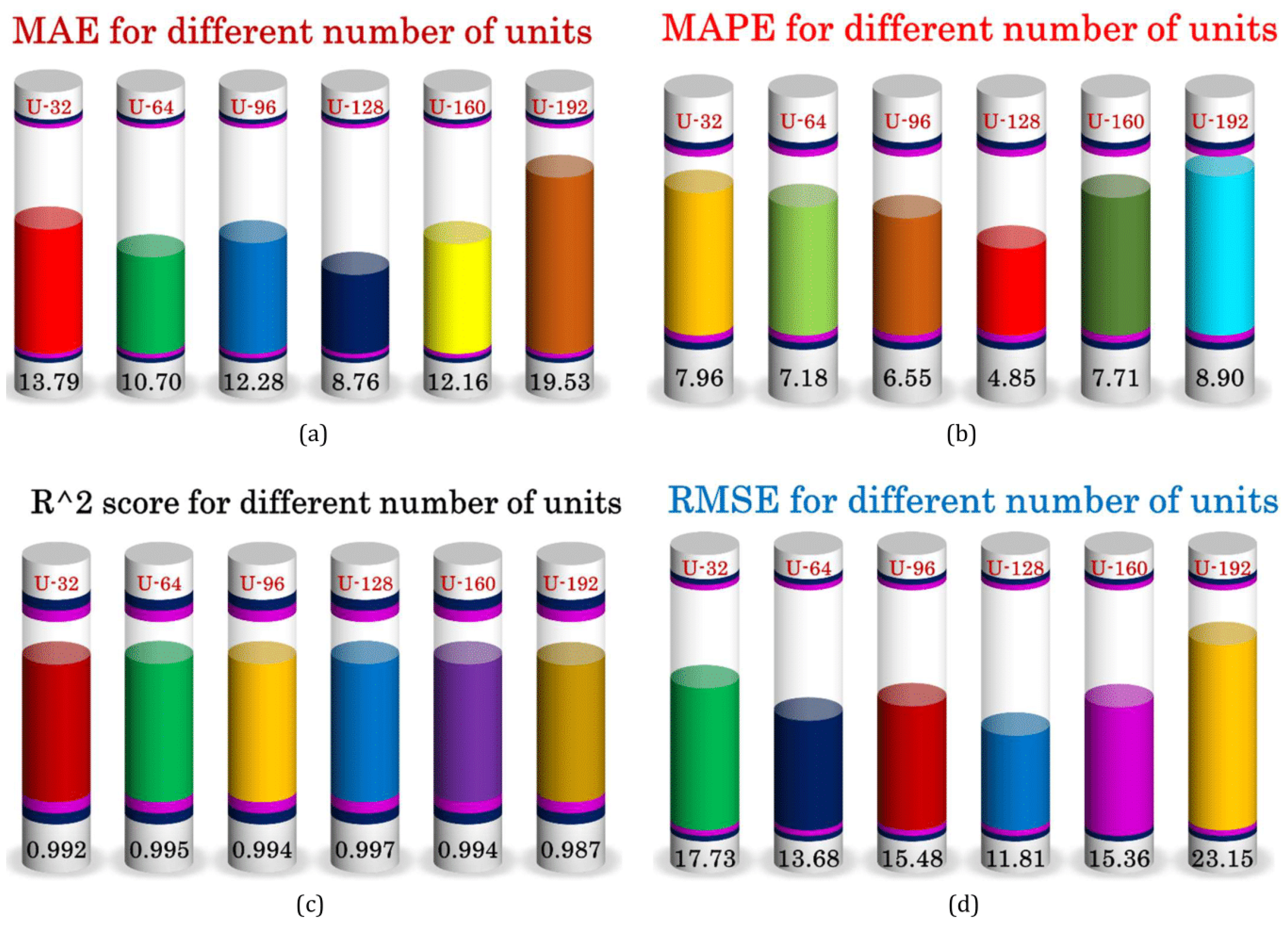
| No. of Units | 32, 64, 96, 128, 160, 192 |
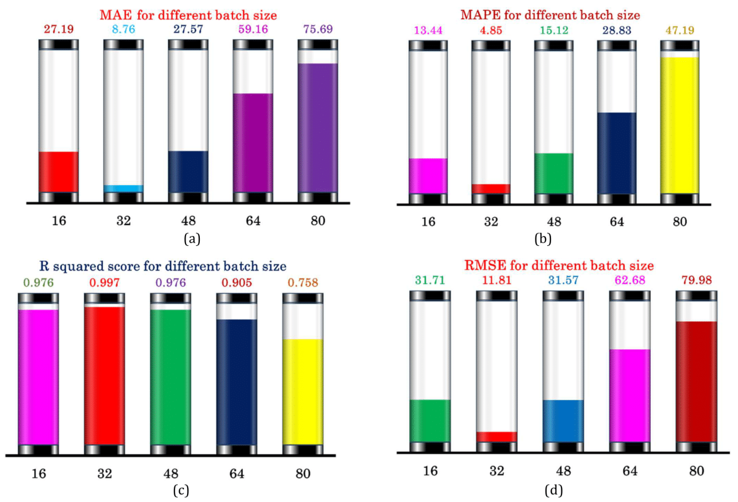
| Batch Size | 16, 32, 48, 64, 80 |
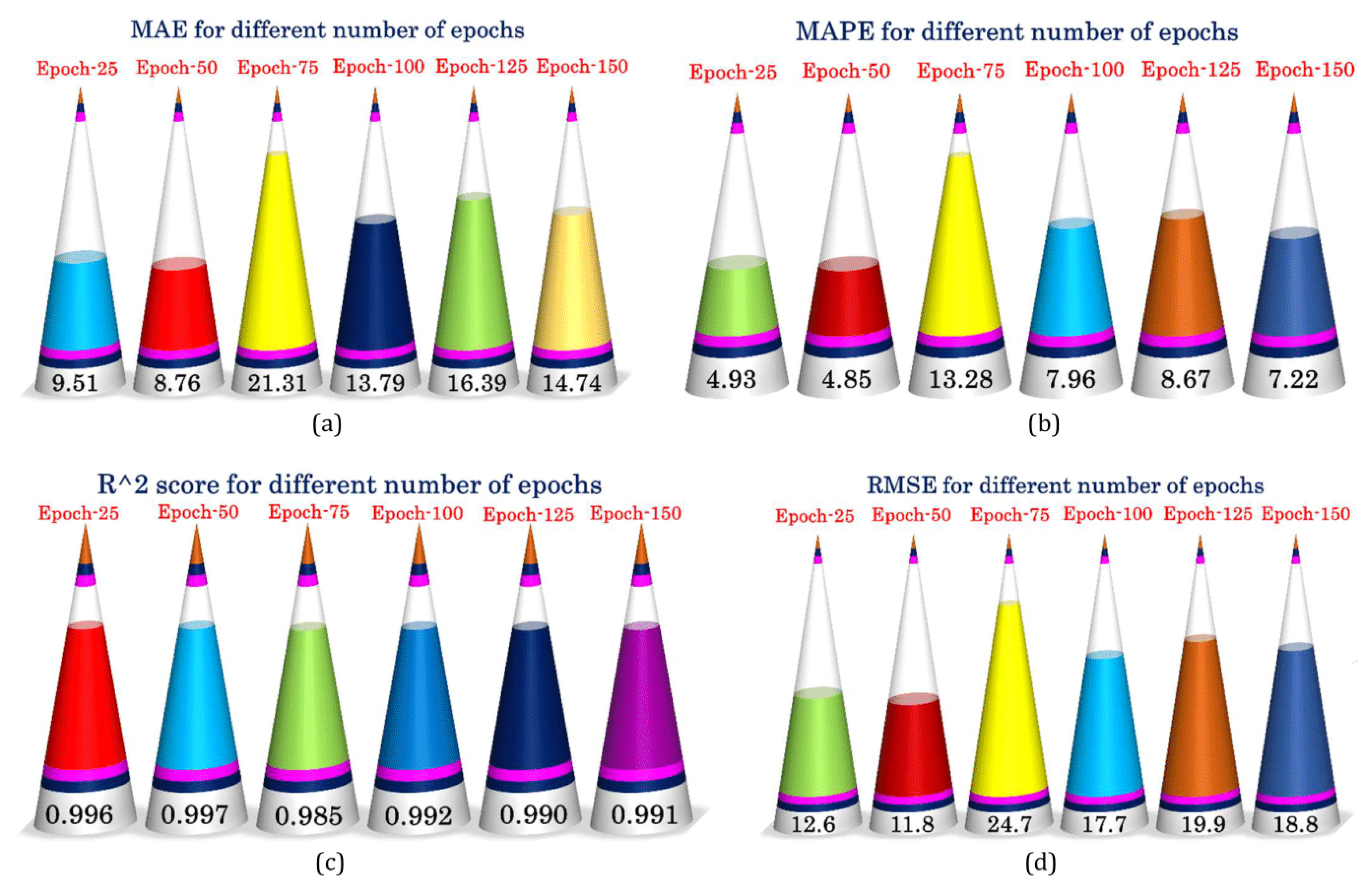
| No. of Epochs | 25, 50, 75, 100, 125 |
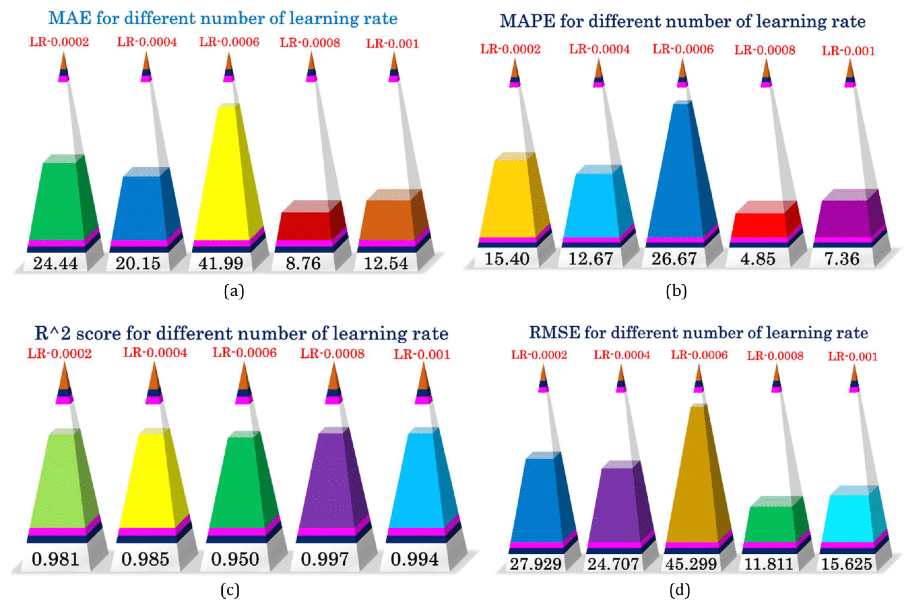
| Learning Rate | 0.0002, 0.0004, 0.0006, 0.0008, 0.001 |
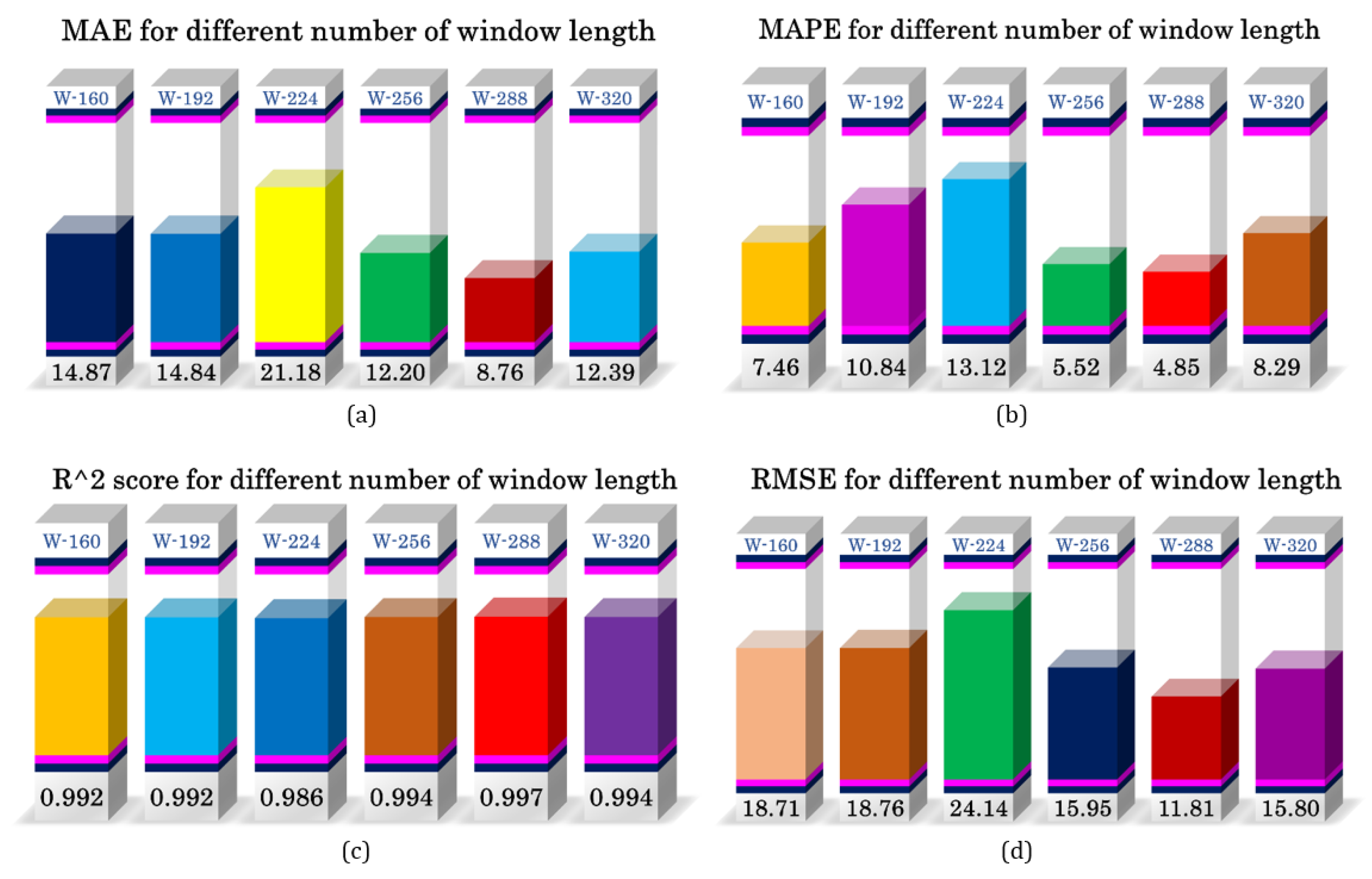
| Window Length | 160, 192, 224, 256, 288, 320 |
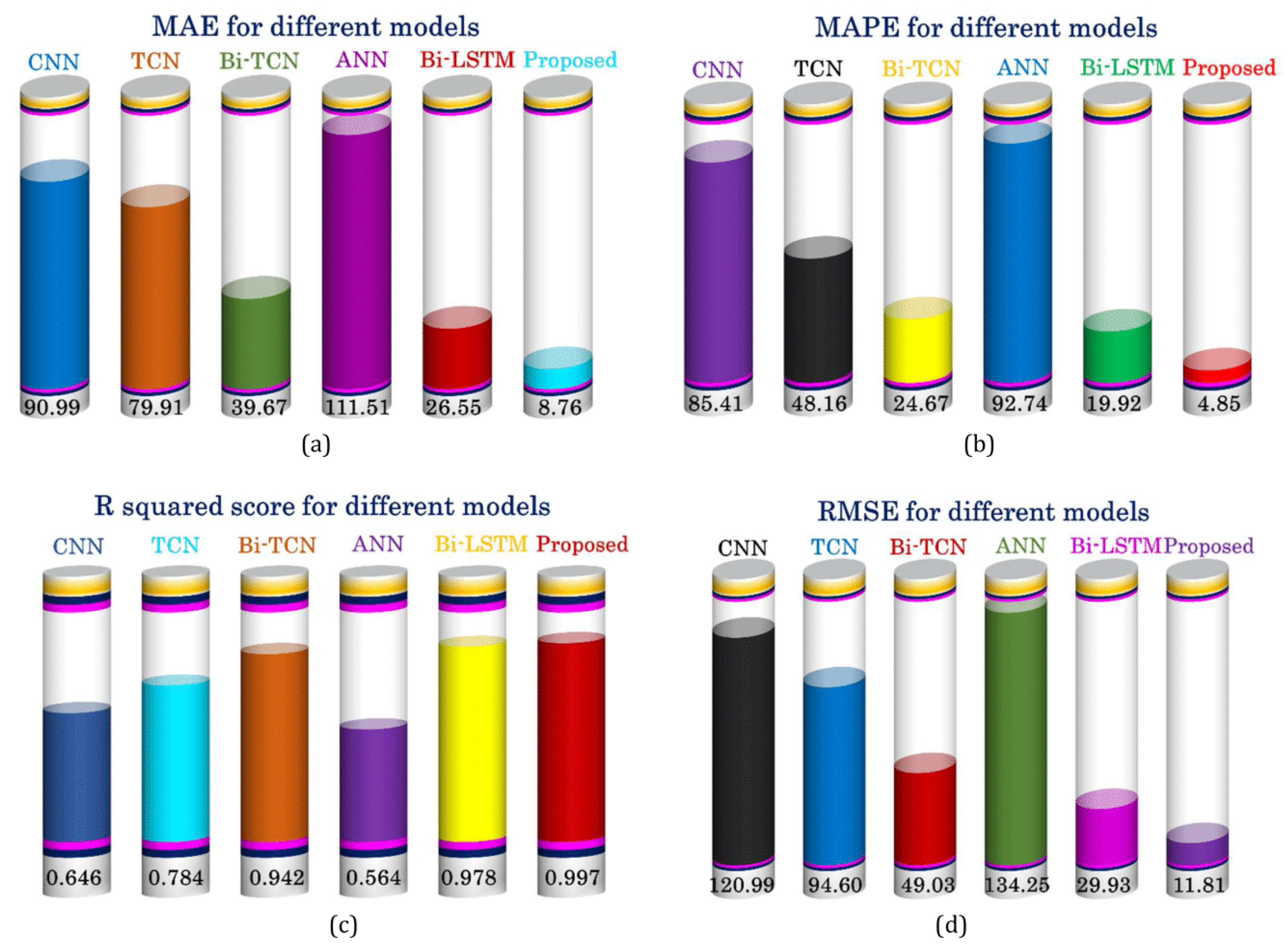
| Section | Attributes/Metrics | CNN | TCN | Bi-TCN | ANN | Bi-LSTM | Proposed |
|---|---|---|---|---|---|---|---|
| Model | Units | 128 | 64 | 128 | 128 | 64 | 128 |
| Learning rate | 0.0008 | 0.0008 | 0.0008 | 0.0008 | 0.0008 | 0.0008 | |
| Epochs | 100 | 100 | 50 | 75 | 100 | 50 | |
| Window length | 288 | 288 | 288 | 288 | 288 | 288 | |
| Batch size | 32 | 32 | 32 | 32 | 32 | 32 | |
| Performance | MAE | 90.98 | 79.90 | 39.67 | 111.51 | 26.55 | 8.76 |
| MAPE | 85.41% | 48.16% | 24.67% | 92.74% | 19.92% | 4.85% | |
| MSE | 14638 | 8948.9 | 2403.5 | 18024 | 895.5 | 139.49 | |
| RMSE | 120.99 | 94.60 | 49.03 | 134.25 | 29.92 | 11.81 | |
| R2 score | 0.645 | 0.783 | 0.942 | 0.564 | 0.978 | 0.997 |
Disclaimer/Publisher’s Note: The statements, opinions and data contained in all publications are solely those of the individual author(s) and contributor(s) and not of MDPI and/or the editor(s). MDPI and/or the editor(s) disclaim responsibility for any injury to people or property resulting from any ideas, methods, instructions or products referred to in the content. |
© 2024 by the authors. Licensee MDPI, Basel, Switzerland. This article is an open access article distributed under the terms and conditions of the Creative Commons Attribution (CC BY) license (https://creativecommons.org/licenses/by/4.0/).
Share and Cite
Habib, M.A.; Hossain, M.J. Revolutionizing Wind Power Prediction—The Future of Energy Forecasting with Advanced Deep Learning and Strategic Feature Engineering. Energies 2024, 17, 1215. https://doi.org/10.3390/en17051215
Habib MA, Hossain MJ. Revolutionizing Wind Power Prediction—The Future of Energy Forecasting with Advanced Deep Learning and Strategic Feature Engineering. Energies. 2024; 17(5):1215. https://doi.org/10.3390/en17051215
Chicago/Turabian StyleHabib, Md. Ahasan, and M. J. Hossain. 2024. "Revolutionizing Wind Power Prediction—The Future of Energy Forecasting with Advanced Deep Learning and Strategic Feature Engineering" Energies 17, no. 5: 1215. https://doi.org/10.3390/en17051215