Floating Offshore Photovoltaics across Geographies: An Enhanced Model of Water Cooling

Abstract

Solar photovoltaics (PV) continues to grow rapidly across the world and now accounts for a very considerable proportion of all non-fossil-fuel electricity. With the continuing urgency of greenhouse gas abatement, the growth of solar PV is inevitable. Competition with other land uses and the desire to optimize the efficiency of the panels by making use of water cooling are compelling arguments for offshore floating PV (OFPV), a trend that could also benefit from the existing infrastructure recently built for offshore wind farms. Building on our earlier work, we present a larger dataset (n = 82) located around the globe to assess global yield (dis)advantages while also accounting for a modified form of water cooling of the offshore panels. Using our results regarding the Köppen–Geiger (KG) classification system and using a statistical learning method, we demonstrate that the KG climate classification system has limited validity in predicting the likely gains from OFPV. Finally, we also explore a small subset of sites to demonstrate that economics, alongside geography and technology, impacts the feasibility of locating PV panels offshore.

1. Introduction

Solar photovoltaics (PV) presently account for roughly 28% of the total of 3.07 TW of installed renewable energy technologies [1], a fact that reflects both the increased maturity of solar PV as a technology as well as the growing confidence of investors in the performance of solar PV. Indeed, the rate of annual increases in solar PV installation envisaged by certain scenarios could be said to be exponential. While the growth in solar PV installations has been rapid, it is also highly uneven. One of the constraints preventing a more equal distribution of solar PV across the globe is competition for land use with other electricity sources. Competition for land could realistically drive up land prices, adversely impacting solar PV’s levelized cost of energy (LCOE). This would be particularly relevant for countries where there is a limited amount of land, for example, small islands such as Malta [2], or countries like the Netherlands, where there is significant competition for land use, but that also seek to establish self-sufficiency in terms of energy security. Land-based solar PV installation may also adversely impact the proper ecological use of land in many parts of the world [3]. Deploying floating PV (FPV), and especially offshore FPV (OFPV), is a means of avoiding any of these conflicts.

FPV deployed on (freshwater) reservoirs can be used not only to relieve pressure on the use of land but also as a means of preserving the usability of freshwater in reservoirs; in other words, there would be a “co-benefit” of using the “footprint” of the PV panels to shade the water from evaporation, and likewise using the reservoirs as a means of enhancing the performance of the PV panels [4]. Today, FPV as floating PV mounted on freshwater reservoirs accounts for less than 1% of the total installed PV capacity but is growing [5]. In contrast, there is no realistic aim of controlling ocean evaporation through the deployment of offshore FPV due to the sheer size of oceans, but there has been a persistent belief that offshore FPV would utilize the cooling potential of ocean water [6].

We propose in this paper to answer multiple interrelated questions. Firstly, we aim to quantify any advantage difference, in terms of energy yield, when moving a land-based solar PV (LBPV) system to an offshore FPV for a specific location in the world as an extension of our earlier work [7]. Secondly, we analyze the geographical factors associated with this energy yield advantage or disadvantage. For this, we construct and test regression models that establish correlations between the location’s geography and the alterations in PV yield resulting from the relocation of panels to offshore sites.

A development in the understanding of how water can play a role in cooling is presented by Kjeldstad et al. [8]: the authors used experimental data to demonstrate a significant (∼5%) improvement in FPV yield compared to land-based systems based on their findings in an experimental setup deployed in Norway. Crucially, the mathematical model developed by Kjelstad and co-workers allows for heat transfer between the water and solar panels for two distinct pontoon architectures: one in which the panel is essentially in contact with the water and the second where the panel is in contact with a floating pontoon. The former is more effective at achieving cooling and, ergo, enhanced PV efficiency. Inspired by the heat transfer modeling described in the literature [8,9,10,11], we develop a PV cell temperature physics model based on first principles. This is important as the heat transfer between water, air, and the components of a panel is not dealt with by the readily available tools for PV modeling.

We note that the Norway-based model [8] cannot easily be extrapolated to a worldwide context. A slightly different approach was taken by a Korea-based research group where the authors used data based on 20 sets of five-minute interval operations in the year 2013, taken from a floating PV module [9]. Instead of developing a model from first principles, they developed a model for the module temperature of the floating panels based on multivariate linear regression, taking as inputs ambient temperature, water temperature, wind speed, and solar irradiance. The regression model developed was also verified by the authors using their experimental data. However, this research paper was more limited than the paper by the Norwegian researchers as they relied on location-specific results to build their regression model, which cannot be reasonably replicated across all the sites we are interested in.

In contrast, the paper by Rahaman and co-authors [10] compares the results from a total of seven thermal models for the operating cell temperature of water-based panels against verification data taken from a limited but well-defined set of actual data taken from a floating PV panel located on an artificial lake in Brazil. Their paper presents the development of the first four thermal models, each with distinct foundations. These include three models grounded in first principles simulations, namely a “thermal model”, a “simplified thermal model” derived from the first, and a “CFD model” rooted in a computational fluid dynamics (CFD) approach. Additionally, an “empirical” model was introduced, which emulates the regression models previously discussed.

Alongside these, the authors in the Rahaman paper discuss three other thermal models for the cell temperature: introducing the Korean researcher model [9], the Niyaz thermal model [12], and the widely reported Sandia model for simulating the performance of PV panels [13].

Comparing the results from each of the seven models against the time-resolved data they collected from the experimental setup, Rahaman and co-workers demonstrated that the “thermal model” based on a first principles approach of the heat transfer between the panel and its surrounding environment is the most effective at predicting temperature changes. In the simplified version that we implement in the present work, the panel itself is divided into three components with distinct thermal properties: a glass cover combined with an anti-reflective coating (ARC); the solar cell material, essentially entirely of Silicon; and a back sheet.

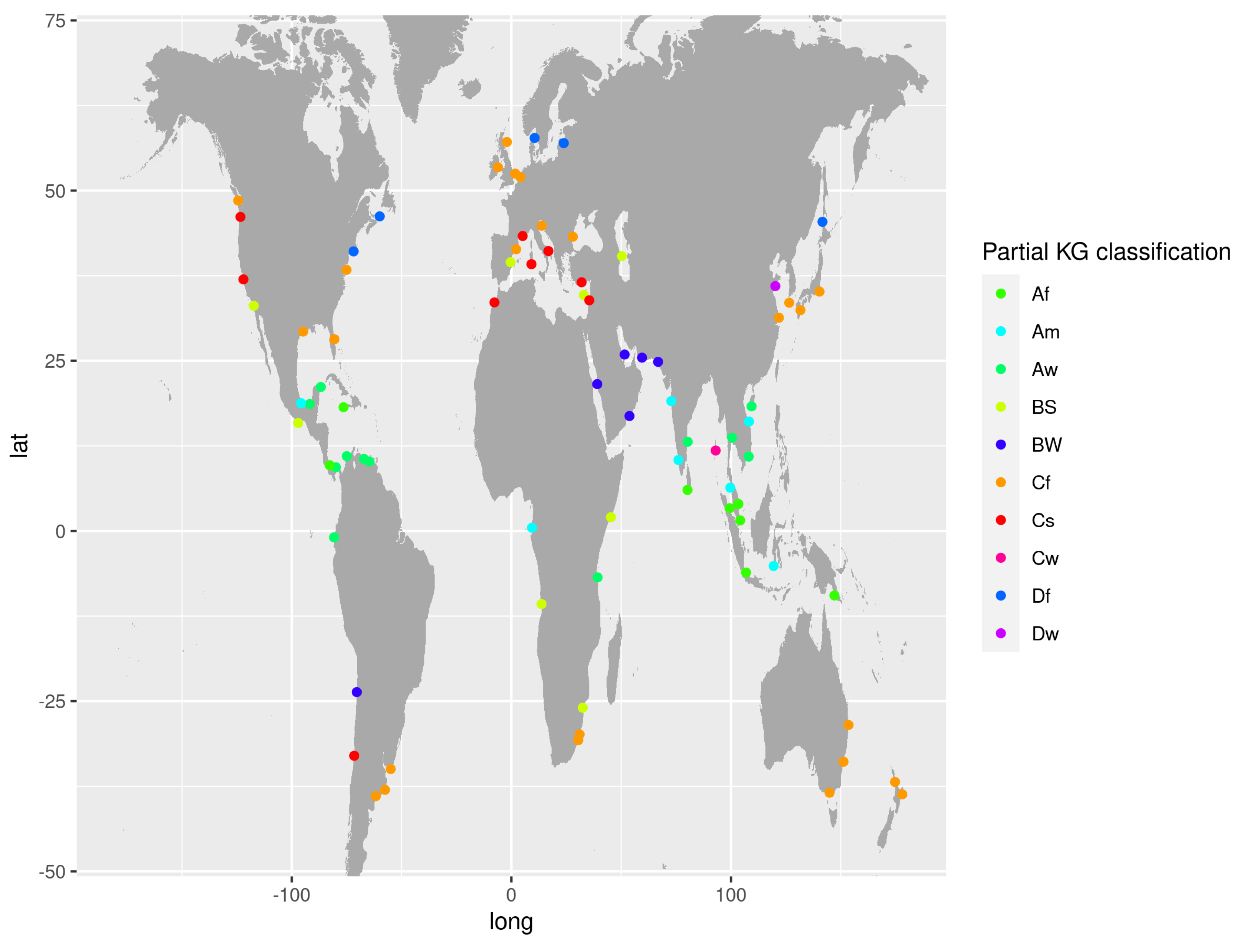
In our earlier work [7], we laid the groundwork for world-scale modeling of the performance of solar PV panels that were placed on offshore pontoons in sites across the globe. In the present research, we will follow the same methodology, but we plan to develop our model and also include additional locations, and make adjustments to the comparative dataset. In this work, each of the modeled offshore sites is chosen to correspond, at a distance generally of ∼56 km, to an arbitrarily chosen major port city around the world. The yield from panels at the offshore site is compared to an equidistant inland site. Together, the offshore site, port site, and inland site represent a “triplet”, of which 82 were initially selected for this work. These are listed in

Table A2. The proportion of hours during which the cell temperature for OFPV is lower than for LBPV, and comparing that to how frequently the water surface offshore was colder than the ambient air inland. A close look shows that the relationship is not simple.

Site Name	TS < T2M (%)	${\mathit{T}}_{\mathit{cell}\mathit{offshore}}<{\mathit{T}}_{\mathit{cell}\mathit{inland}}$ (%)
Jedda (SA)	84	86
Puerto Colombia	81	91
Jod (IR)	78	83
Mogadishu	77	86
Vina del Mar (CL)	77	81
Santa Cruz, CA (USA)	74	86
Puerto La Cruz (VE)	73	87
Ras Laffan (QA)	72	81
Karachi (PK)	71	84
Mughsail Beach (OM)	70	84
Jeju (RK)	67	81
Carlsbad, CA (USA)	66	76
Ocean City, FL (USA)	65	79
Fortalezado do Amboim (AO)	65	83
Dar es Salam (TZ)	64	82
Glace Bay, NS (CA)	64	76
C. del Carmen (MX)	63	79
Montauk Pt., NY (USA)	63	78
Puerto Belgrano (AR)	63	78
Mumbai (IN)	63	83
Bangkok (TH)	63	83
Hengsha Island (CN)	63	86
C. San Salinas (VE)	62	82
Maputo Port (MZ)	62	76
Riga	62	72
El Emir (UY)	62	80
Mar del Plata (AG)	62	78
Baku (AZ)	61	73
Lowestoft (UK)	60	76
Port of Rotterdam	59	77
Qingdao (CN)	59	80
Varna (BG)	58	73
Galveston Island, TX (USA)	56	79
Limassol (CY)	55	75
Howth (IE)	55	75
Port Renfrew, BC (CA)	54	69
Mantahost (EC)	54	83
Port Vell (ES)	53	72
Satellite Beach, FL (USA)	53	79
Caligari (IT)	52	73
Skagen (DK)	51	68
Port Moresby (PG)	51	82
Carry-le-Rouet (FR)	51	72
Cancun (MX)	51	83
Westport, OR (USA)	50	62
Heroica Veracruz (MX)	50	81
Chennai Port (IN)	49	84
Morocco	48	74
Jishy (IN)	48	80
Valencia (ES)	47	67
Melbourne Beach (AU)	45	78
Bari (IT)	42	71
Panama	41	84
Aquarium Pula Croatia	38	68
Libreville (GA)	38	80
Bandar Penawar (MY)	38	84
Bondi Beach (AU)	35	71
Sanya (CN)	35	78
Aberdeen (UK)	32	53
Katsuura (JP)	30	76
Port Antonio (JM)	29	75
Da Nang (VT)	29	71
South Golden Beach (AU)	29	73
Antofagasta (CL)	29	83
Phan Thiet (VT)	27	77
Beirut (LB)	27	66
Langkawi (MY)	27	79
Cooper Reserve (NZ)	24	64
Kantor Makasar (ID)	23	77
Galle (LK)	22	70
uShaka (ZA)	21	67
Port Shepstone (ZA)	18	68
Sitapur (IN)	15	80
Tanjung Priok (ID)	12	77
Miyazaki Port (JP)	11	66
Kaiti Beach (NZ)	9	66
Beihei (CN)	6	60
Kwala Tanjung (MY)	6	72
Alanya Kalesi (TR)	5	53
Kuantan (MY)	1	78
Puerto Escondido (MX)	0	68
Puerto Viejo de Talamanca (CR)	0	70

, in Appendix B, and also shown in the map plot in Figure 1 where they are color-coded using the Köppen-Geiger (KG) classification system [14].

This work advances the earlier work in a number of ways. Firstly, we have increased the number of “site triplets” under investigation from 20 to 85. This enlarged dataset will add more certainty to our earlier findings. Secondly, we have enhanced the thermodynamic modeling of the offshore FPV panels. In this paper, we adopt a 2-D multi-layered approach to simulate the water cooling of the offshore FPV systems. This improvement allows us greater confidence and more robust results in understanding how water bodies impact the operating temperature of FPV. Finally, we move on to examine in greater detail how economic aspects can also impact the financial feasibility of offshore FPV by focusing on pairs of comparable locations.

2. Methodology

Our aim in this paper is to have a more complete understanding of which sites globally are best suited for the deployment of offshore FPV. We first describe the data collection sources before moving on to the computational techniques we used. In Section 2.2, we describe our general approach to constructing “triplets” of sites and how they fit into our wider modeling approach. Later, we move on to describe our first principles approach to modeling the operating cell temperatures of the offshore FPV. Results will be presented in Section 4, followed by a discussion of their importance in Section 5. Our main findings are that the desirability of using offshore FPV varies from one site to the next; that that desirability can be quantified by determining the likely advantage in the yield of PV panels we can expect from siting PV panels offshore; and that currently available geographic classifications do not provide us with a straightforward means of determining the best sites to deploy offshore FPV.

Supplementary data and information can be found in Appendix A and Appendix B, and the codes will be provided online (GitHub) as appropriate.

This paper aims to present a quantitative and statistical comparison between LBPV and OFPV and to tie these findings to geographic and economic realities. Performance modeling of land-based PV systems has been well-established for some time, and PVLIB, an open-source Python library, is well-documented [15]. Results for the LBPV systems reported in this paper rely on PVLIB, and this is detailed in Section 2.3.1.

2.1. Data Collection

All of our data are based on a 10-year period, from 1 January 2008 until 31 December 2017, using hourly time resolution and derived from satellite images (NASA POWER [16]).

Table 1. Different parameters used for the technical calculations.

Parameter	Definition	Comments
T	The ambient temperature at 2 m height	Used for all sites
$T_{sea}$	Sea surface temperature	Used for offshore sites, informs cooling of panels
$G_{Diff}$	Clear sky diffuse radiation	Is computed together with the Clear sky Index, $K_t$
$K_t$	Clear sky index, clearness index	Informs $G_{Diff}$ together with the GHI under clear sky conditions
$GH{I}_{CLRSKY}$	The GHI under clear sky conditions
$P_r$	Total precipitation, corrected	Used for testing the previous regression model
$G_{GHI}$	Global Horizontal Irradiance	Used as one component to calculate the plane-of-array (POA) irradiance
$v_w$	The wind speed at 2 m height	Used to inform solar cell operating temperature

provides the list of variables that we downloaded and used to calculate the results in this paper.

As with any dataset based on satellite imagery, it is important to understand the limitations imposed on the data by the uncertainty in the measurements. Ultimately, NASA POWER is built on a series of long-standing satellite imagery initiatives managed by NASA [16]. More importantly, work to validate the findings of NASA satellite imagery against the ground- and sea-based observations has shown that any biases are moderate and are not systematic (i.e., are not tied to location) [17]. Finally, it should be noted that the NASA POWER dataset remains the only single dataset that can provide information on a given site, offshore and inland, and which is also freely available. All these combined suggest that it is the right dataset for the purposes of this paper.

Building “Triplets” of Sites

Our original dataset included a total of 82 arbitrarily chosen ports from around the world. These include 20 sites that we reported on in the previous paper [7], and 62 added to it. To go from a single port site to a “triplet” that includes a port and equidistant offshore and inland sites, we first determine what the “direction of travel” is for the port. This is simply defined as the cardinal direction in which a boat leaving that port takes; for example, if the port is on the shoreline of North Africa, a ship leaving that port would likely have to face north, towards Europe, to leave, and this is the direction of travel to reach the next site. Next, we determine what the difference in longitude and/or latitude would be for sites to be within ≈56 km from the original site. Note that, when sites are moved longitudinally (i.e., moving along an east–west axis), then the distance moved varies as the cosine of latitude (thus, at the poles, there is no distance between degrees longitude).

2.2. Geographical Classifications: Understanding the Role of the Köppen–Geiger System

The most widely recognized system for the classification/codification of the climate of specific locations is the Köppen–Geiger (KG) climate classification system. Briefly, the KG system divides any location according to three different levels. The first divides the world into five (5) different zones, essentially replicating systems of climate classification that existed in medieval times or earlier: these range alphabetically from “A”, equatorial, to “E”, polar climate, zones. The second level codifies the amount and general pattern of precipitation; these range from “W” for desert to “m” for monsoonal. Finally, a third—not always present—level of classification categorizes a given site by a typical temperature; these range from “h” for “hot arid” to “d” for “extremely continental” [18].

For our work, we rely on the HDD (“Hydrological Data Discovery”) Tools package [19] (version 0.1.1), which, given a pair of longitude/latitude coordinates, will return a full classification of the given site. For example, the site in northern Qatar has a KG classification of “BWh”, which indicates that it is an arid site, with a desert level of precipitation and a high average temperature. Meanwhile, Sella, a site in Italy that is also in our dataset, has a KG classification of “Csa”, which signifies that the site is in a temperate climate zone (“C”) and that the general weather pattern is “warm” (“s”) with a dry summer pattern of precipitation (“a”).

Importantly, the HDD Tools package can return multiple categories of KG classifications for a single site; this results from the fact that HDD Tools samples a region (a “bounding box”) around a specific pair of coordinates, therefore allowing for multiple classifications. We explain in Section 4.4 how we deal with this uncertainty in more detail. Based on earlier work, one of the main hypotheses of our paper is that the KG climate classification does not help to inform the optimization of siting OFPV: we do not expect that a given port site’s KG climate classification will be an indication of the scale of offshore advantage, or even if there is an offshore advantage.

We try to test our hypothesis by classifying the yield advantages using a statistical learning method and then comparing the output to the original KG climate classification. This approach emulates, partially, that of the “data-driven” climate classification reported by Lasantha and co-workers [20], where sites across the world are classified according to a number of meteorological and topographical determinants using unsupervised statistical learning methods.

2.3. Modeling the Operating Cell Temperatures

The conversion efficiency of a PV cell is inversely related to the cell’s operating temperature, itself a function of the ambient temperature. In this paper, our results are derived by comparing the cell temperatures obtained through two distinct methods: one for the land-based (port-based and inland) sites and another for the offshore sites.

2.3.1. Modeling the Land-Based System

In our earlier work, we substituted the normal ambient (2-m) temperature with a “heat index” temperature [21,22]. The heat index temperature is based on a regression model developed in the 1970s and is computed as a function of the ambient temperature and the relative humidity. Using a much larger dataset, however, we found that substituting the heat index for the ambient air temperature resulted in asymptotically high cell temperatures in multiple locations.

In this paper, we modeled the cell temperature of the land-based PV panels by using the widely cited Sandia PV Array Performance Model [13], implemented through Python’s PVLIB [15] library, which we will refer to throughout this paper as the “PVLIB model” or “PVL”. This approach takes (plane of array, POA) solar insolation, ambient air temperature, and wind speed to compute the output of the PV modules. We also assume an insulated back glass/polymer solar module.

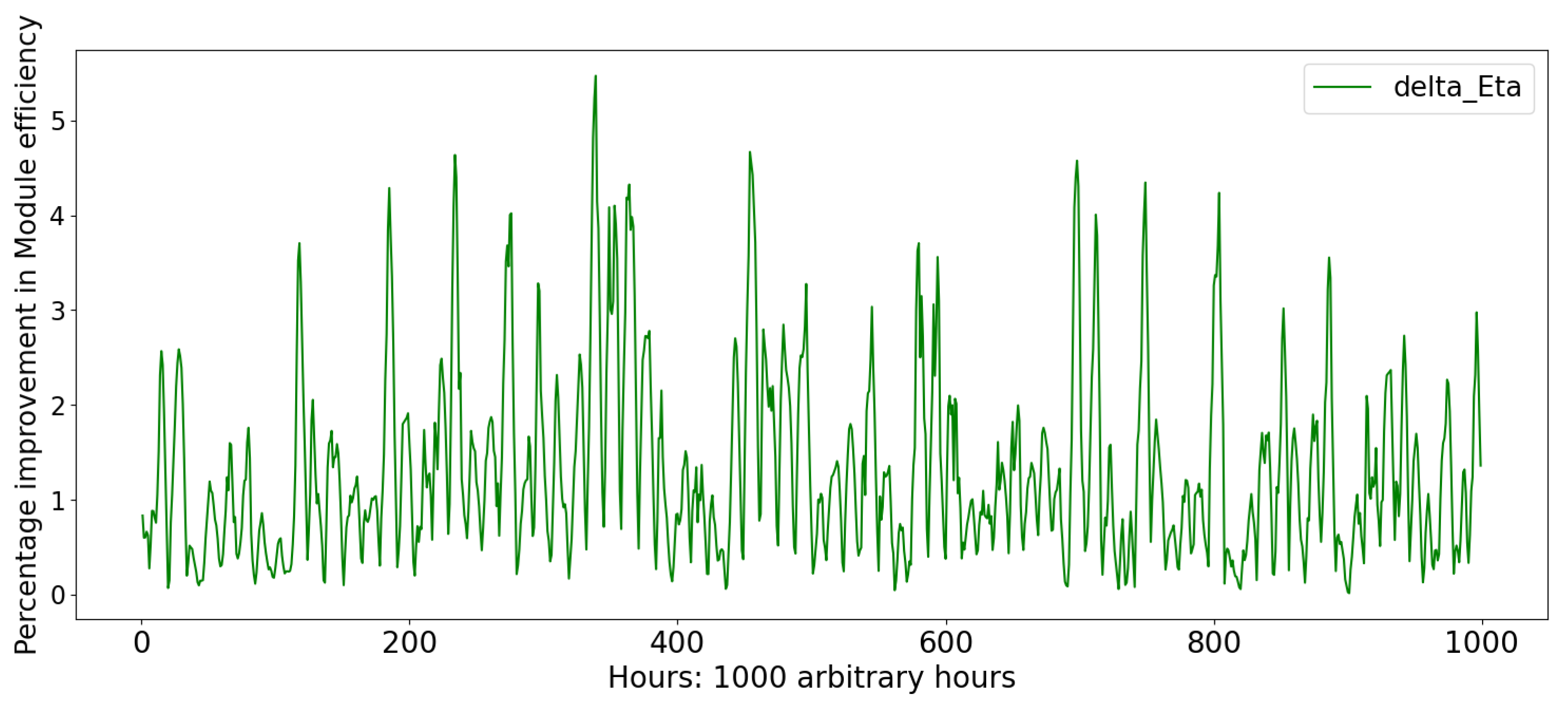
We illustrate the importance of including wind speed as a factor in the cell temperature within the PVL model in Figure 2, where we model how the module efficiency is affected when we take the wind speed (at 2 m height) into account. The data are taken from the Cooper Reserve site in New Zealand, where the inland site had the highest average wind speed. We took a subset of 1000 h when there was enough insolation for us to count the output (>50 W/m²).

Importantly, once we calculate the cell temperature for the OFPV panels, we continue to use the same SAPM paradigm through PVLIB to calculate the efficiency of the modules and the output, allowing us to more directly make comparisons needed.

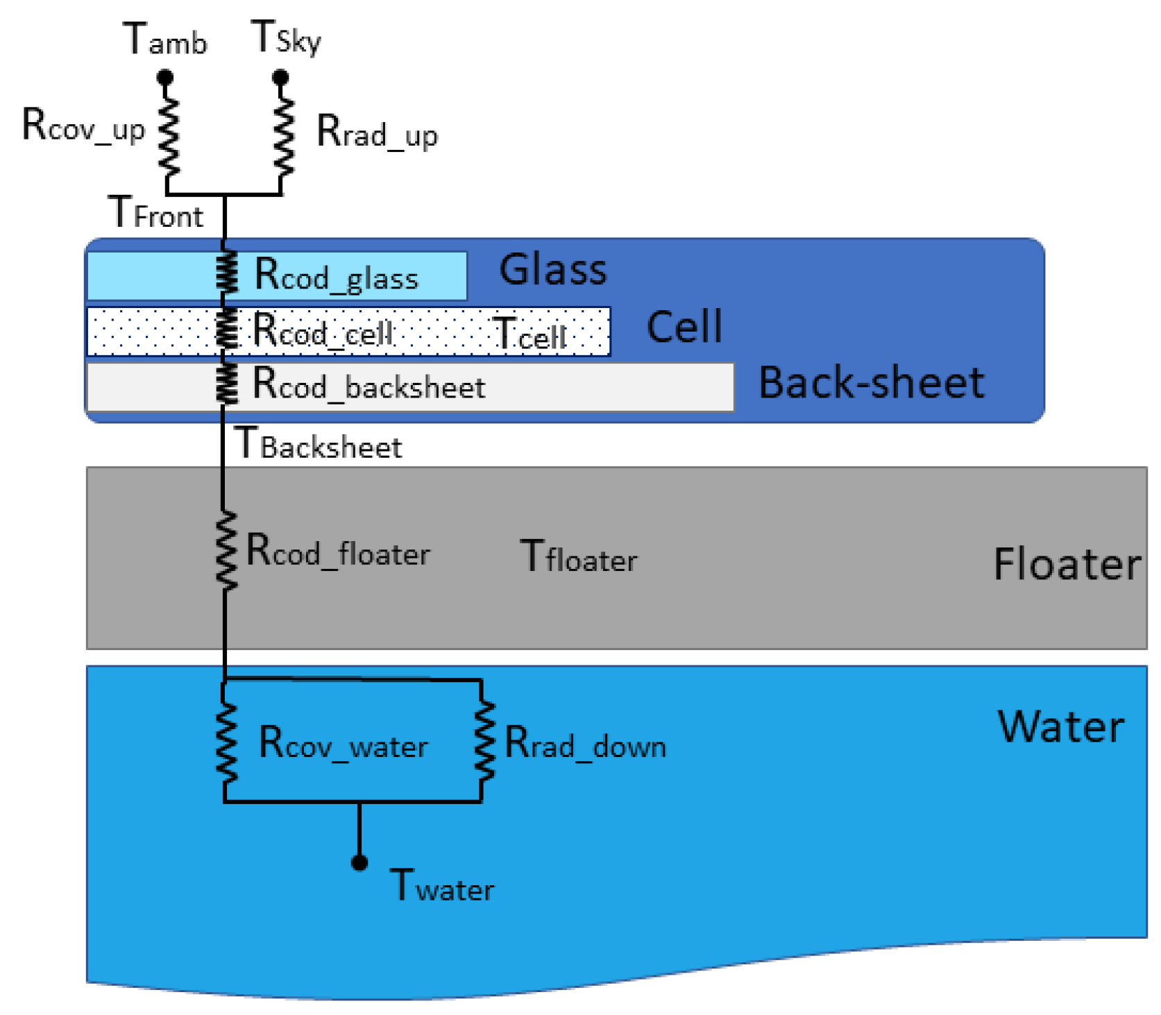
2.3.2. Cell Temperatures for OFPV Panels: A Simplified Adaptation

For the LBPV systems both in the inland sites and the port sites, we rely on the meteorological data downloaded to calculate the back of module temperatures, cell temperatures, and module efficiencies using the SAPM (Sandia Array Performance Model). Yet, as has been demonstrated in [8] as well as [9] and several others, this is not necessarily applicable to the offshore panels. Specifically, we assume that the offshore structure is a pontoon concept that makes the offshore panels essentially in thermal contact with the open water from their back sheet; see Figure 3.

As with the approach described in [10], we model the heat transfer between the panels and the surrounding environment as being dependent on three independent ordinary differential equations (ODE):

1.

The time-dependent ODE governing the heat transfer between the front of the panel, the air, and the silicon panel:

$$P_S+Q_{conduction,F}+heat-Q_{convection,F}-Q_{radiation}=m_{glass}\times C_{glass}\times \frac{d{T}_{Front}}{dt}$$

(1)

where $P_S$ is the irradiation power absorbed by the front of the PV panel. $Q_{conduction,F}$ is the conductive heat transfer from the cell to glass cover. $Q_{convection,F}$ is the convective heat transfer from cover to ambient, $Q_{radiation}$ is the radiative heat transfer from cover to sky, $mas{s}_{glass}$ is the mass of the glass, $C_{glass}$ is the heat capacity of the glass, and $T_{Front}$ is the temperature of the front of the module.

We can see from the right-hand side of this equation that this is simply the heat energy absorbed by the glass sheet itself, used to increase its temperature. On the left-hand side of the equation, we can see that the time-dependent amount of energy absorbed is based on the total electromagnetic energy (essentially sunlight) absorbed by the surface of the front of the panel, in addition to the energy that is radiated “upwards” by conduction from the cell and the amount of heat energy lost by the cell. From this, we subtract the heat that is lost to the surroundings by convection (generally through wind cooling) and the amount of energy that is radiated up to the sky (through reflection).

2.

An ODE governing the heat transfer between the silicon material and the front and back sides of the panel, which is provided by

$$-P_e-Q_{conduction,upanddown}+Q_j={\mathrm{mass}}_{\mathrm{silicon}}\times C_{silicon}\times \frac{d{T}_{cell}}{dt}$$

(2)

where $P_e$ is the electrical power developed by the PV cell, $Q_{conduction,upanddown}$ is conductive heat transfer from cell to glass, $Q_j$ is Joule heating, ${\mathrm{mass}}_{\mathrm{silicon}}$ is the mass of the silicon, $C_{silicon}$ is the heat capacity of the silicon, and $T_{Cell}$ is the temperature of the solar cell in the module. Equation (2) can be understood in a similar fashion to Equation (1) above. On the RHS, we have the total energy needed to instantaneously raise the temperature of the silicon cell. The energy available to change the temperature of this cell is thus $Q_j$ less the energy used to drive electrical power ($P_e$), as well as the conduction of energy both to the front and back of the panel. In turn, the heat energy $Q_j$ is provided as a function of the resistance of the silicon material, as per [10]: $Q_j=I^2\ast R_s+\frac{V^2}{R_{sh}}$ where the R values are the series and shunt resistance values, respectively.

3.

A third equation governs the heat transfer provided as a function of the transfer between the back of the module, the cell, and then the contact. In our case, this contact is entirely with the pontoon (since the panels are horizontal, tilted at a 0-degree angle):

$$\begin{array}{c}\hfill Q_{conduction,celltoback}-Q_{conduction,down}-Q_{ra{d}_{down}}-Q_{Con{v}_{d}own}=\\ \hfill mas{s}_{backcover}\times C_{back}\times \frac{d{T}_{Back}}{dt}\end{array}$$

(3)

where $Q_{conduction,celltoback}$ is the conductive heat transfer from cell to back sheet, $Q_{conduction,down}$ is the conductive heat transfer from back to the water, and $Q_{ra{d}_{down}}$ is the radiative heat transfer from back sheet to water, and $Q_{Con{v}_{d}own}$ is convection heat transfer from floater to water, $mas{s}_{backcover}$ is the mass of the back cover, $C_{back}$ is the heat capacity of the back sheet, and $T_{Back}$ is the temperature of the back side of the module.

In contrast to the model reported in [10], we make a minor adaptation to the modeling of the convection component of the modeling, which impacts both the air cooling of the front panel and the water cooling of the back of the panel. Specifically, where [10] makes a distinction between free and forced convection, we concerned ourselves with only free convection. Secondly, where the authors of [10] used a formally established convection equation, we chose to use a simplified model found in the literature that calculates a heat transfer coefficient as a linear model based purely on wind speed.

For our purposes, we simplified all calculations dealing with convection, assuming that all flow would be non-turbulent. We simply defined the convective heat transfer coefficient to be a linear function of wind speed. This linear interpolation can be found in [23] (Figure 2). We define all convection to be a linear function of the wind speed, expressed in m/s:

$$Q=f\left(w_{speed}\right)\left\{\begin{array}{cc}8\hfill & \mathrm{if}{v}_w=0\hfill \\ 8+2\frac{1}{3}\times v_w\hfill & \mathrm{if}0<v_w<6\hfill \\ 25\hfill & \mathrm{if}{v}_w\ge 6\hfill \end{array}\right.$$

(4)

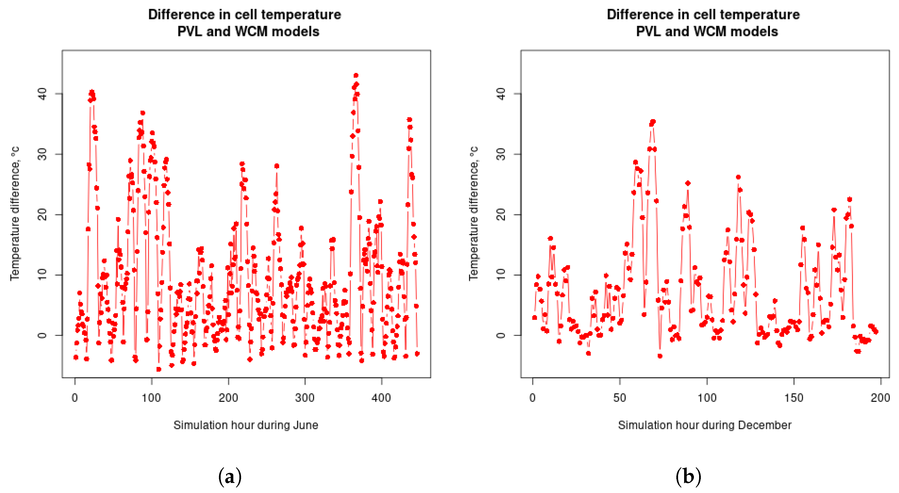
While this is a very considerable simplification, we believe it is justified in our case as the situation described by [23], of horizontal windows protected by a vertical wall, could be readily translated to our situation of floating offshore solar panels. We then solve each of these three equations simultaneously using Python’s ODEINT within the SciPy (version 1.11.3) library [24], for each hour in the dataset. In each successive hour, we take as the initial condition the temperature solved for the preceding hour (e.g., at hour 4000, the front-of-module temperature is equivalent to what was solved for at hour 3999). During our initial hour (hour 1 of 87,672 h), we assume that the front of the panel and the glass are at the temperature of the air; that the back of the panel is at the temperature of the water; and that the cell itself is at the average of these two temperatures. The differences in the two models can be illustrated graphically. We first define a simple $\delta T_{cell}=T_{cell,PVL}-T_{cell,WCM}$. We note that the sign of the difference here is significant. We then look at those values for the specific months of June and December, 2013 for the offshore site associated with the port of Rotterdam and only consider hours with significant insolation. The results are displayed in Figure 4.

Here, we found that the PVL produces a cell temperature lower than the WCM only between 15% and 17% (December and June, respectively) of all the significant hours. Graphically, it is also apparent that, during the majority of hours when the PVL produces a higher temperature than the WCM, the scale is much greater.

2.4. Calculating the Results

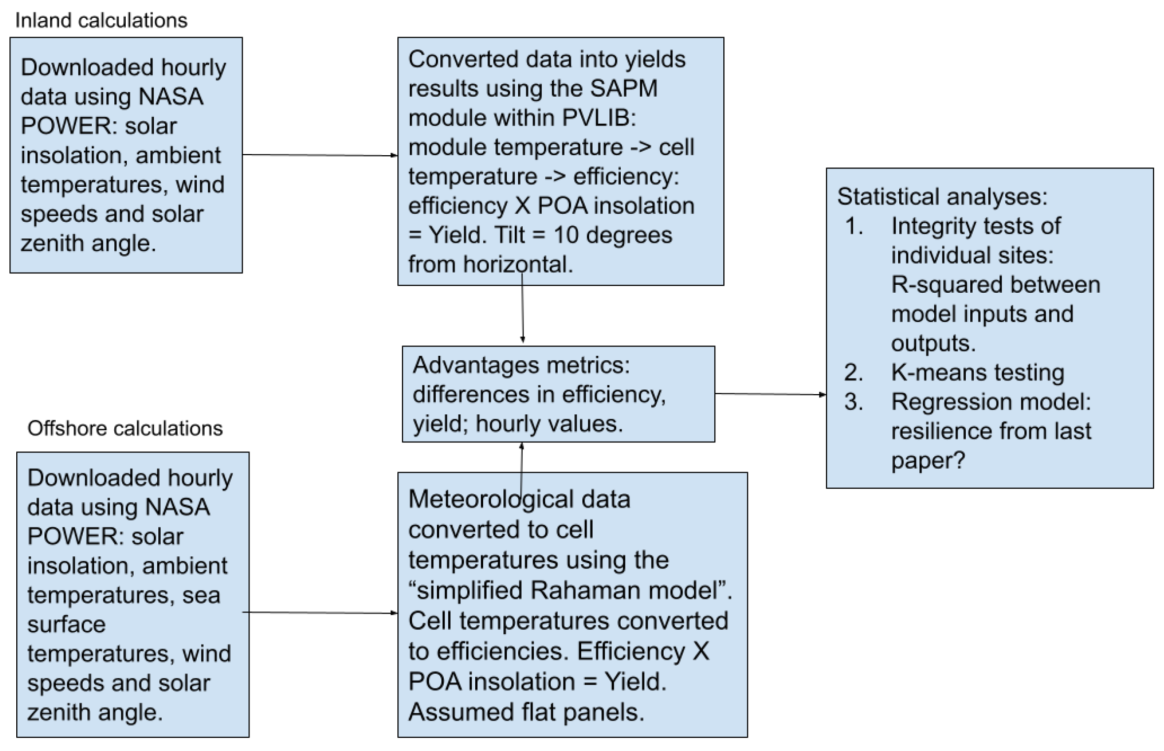
As illustrated in the flowchart, Figure 5, the chain of modeling in our system worked as follows:

1.

For the LBPV: We assume that the solar panels are tilted by 10° from the horizontal. This was completed to provide all the LBPV panels an equal footing for comparison, without having to model a specific solar irradiance model. We calculate the total amount of irradiance on the panels given the different components of solar irradiation (direct and diffuse). The results from the PVLIB “get total irradiance” from within the “irradiance” module are then used to calculate the “plane of array” (POA) irradiance, at an hourly resolution. We are able to combine the POA irradiance with the ambient temperatures and wind speeds to generate a temperature of the PV panel. This is completed using the SAPM implementation in PVLIB. To calculate an hourly yield, we simply compute $Y=\eta \ast G_{POA}/G_{STC}$, where $G_{POA}$ is the POA irradiance and $\eta$ is the calculated efficiency. $G_{STC}$ is taken to be 1000 W/m².

2.

For the OFPV: We assume that the panels are horizontally tilted (0°). We calculate the POA irradiance using the same approach as described for the land-based panels. The POA irradiance is fed into the method described in Section 2.3.2.

We provide in

Table A3. Thermal and other material properties that we used for our calculations. All data reproduced from [10].

No.	Material/Parameter	Thickness	Thermal.Conductivity	Density	Transmission	Absorption	Emissivity	Specific.Heat
1		m	W/(m × K)	kg/m3				J/(kg × K)
2	Glass cover	0.003	1.8	3000	0.95		0.91	500
3	ARC layer	100 × (10−9)	32	2400				691
4	Si cell	255 × (10−6)	148	2330		0.85	0.70	677
5	EVA layer	500 × (10−6)	0.35	960				2090
6	Tedlar back sheet	1 × (10−4)	0.2	1200			0.85	1250
7	HDPE plastic	0.1 × Area	0.48
8	air	–	0.025	1.25				1.256
9	Sky	–	–				0.91
10	Water	–	0.57	1000			0.95	4186

the material properties of the modeled OFPV panels. The thermal resistances are particularly important to the outcomes of the modeling of the offshore panels.

2.5. Limitations to OFPV

While this paper presents a model for the performance of OFPV in many sites across the globe, it is imperative to point out that there are serious considerations before any effort can be attempted to deploy PV panels offshore. The first is the simple matter of novelty: to date, floating PV as a whole accounts for roughly 1% of total worldwide and, within this, OFPV remains an essentially negligible proportion. This novelty on its own will make financing efforts for OFPV more difficult, if only at first.

Second is the need to develop robust and test-proven pontoon structures that can be shown to maintain functioning OFPV panels. It should be noted that much of our modeling is dependent on a high-conducting (metallic) pontoon. Leaving aside any economic considerations, this poses considerable logistical and technical challenges to ensure that the correct infrastructure can be sourced and placed at appropriate distances offshore. While we do not anticipate that any floating offshore pontoons will be capsized due to wind/storms, damage to the offshore panels due to flying debris remains a distinct risk.

In summary, the major limitations to OFPV remain those to do with the cost of building waves or storms; damage to the panels from flying debris remains a real concern for novel infrastructure, as well as understanding how it will integrate with existing offshore infrastructure and how it can be placed to avoid maritime traffic.

3. Quantifiable Results

The results for this project come in the form of cell temperature structure, which remains stable in mores and effisolar installations, and OFPV is still in its infancy. This alone presents some efficiencies and PV yields for each pair of offshore and inland sites. In the subsections below, we outline what the metrics we measure shall be and how these will provide us an indication of the success or otherwise of our hypothesis.

3.1. Previous Regression Model: Robustness

In Ref. [7], we presented an overall regression model that fit the dataset used at the time (composed of 20 locations) and which allows users to predict with a high degree of accuracy (i.e., with an R-squared value of ∼98%) the relationship between the yield advantage and specific meteorological data:

$$\Delta \widehat{E}={\alpha }_0+{\alpha }_1\ast \Delta G+{\alpha }_2\ast P_r+{\alpha }_3\ast T_s+{\alpha }_4\ast \Delta v_w$$

(5)

Here, the notation $\Delta \widehat{E}$ is used to designate that we are examining the predicted values. In this case, we are trying to predict the value of the difference in energy yield as a function of four meteorological factors: the solar irradiation difference between the offshore and inland sites $\Delta G$, the precipitation $P_r$ is the overall total precipitation on the associated port site within the triplet, $T_s$ is water surface temperature, and the wind speed difference between the offshore and inland site $\Delta v_w$.

In Section 4, we will judge the success rate of the above model to the extent that the model in Equation (5) is able to predict the outputs of our expanded dataset.

3.2. Cell Temperatures, Efficiency

Cell temperatures are the main determining factor of the efficiency of a PV panel. While the cell temperatures of the PV panels are calculated in different ways for the offshore and land-based systems, the efficiency of the panels is based on the same ADR (current, diode, and resistor) model [25] in PVLIB, which we will term the PVL model. The full exposition of this model for module efficiency is detailed in a 2020 technical report by Driesse and Stein [26], which models module efficiency as a function of the normalized irradiance (here symbolized S) and the (cell) temperature, $\eta (S,T)$:

$$\eta (S,T)=k_a\ast [(1+k_{rs}+k_{rsh})\ast v(S,T)-k_{rs}\ast S-k_{rsh}\ast v{(S,T)}^2]$$

(6)

In Equation (6), the values $k_a,k_{rs},k_{rsh}$ are fitting parameters describing the initial conditions, series resistance, and shunt resistance, respectively. We note that the authors of the ADR model have demonstrated that it has a lower level of error compared to other models meant to determine the efficiency of a PV module. Readers interested in the full exposition of this model are invited to examine the literature.

To quantify the differences between competing models for the cell temperatures of the offshore FPV panels, we provide in Section 4.3 the outlines of how our derived water cooling method (WCM) compares against the PVL model, which relies on solar insolation, ambient temperatures, and wind speeds to determine the operating temperatures of the modules/cell temperature.

We will provide two different ways of quantifying the results. First, we look at how the hour-by-hour cell temperatures for the offshore and inland sites within a given triplet compete. This compares the OFPV cell temperatures, where we rely on the WCM method, and the LBPV cell temperatures, where we will always rely on the PVL method to determine the cell temperature.

In the second approach, we hold the weather patterns constant and compare the output of the PVL cell temperature and WCM temperature for the same set of offshore sites. In this approach, we are able to focus more closely on the performance of the WCM as a means of determining cell temperature.

3.3. PV Yield

While PV efficiency is a good proxy for the performance of PV panels, the global nature of our dataset also means that the simulated yield from the panels is an additional and important metric for the performance. This is because sites, whether offshore or land-based, may have a high level of efficiency for a given hour, but it might be offset by a low level of irradiation, or vice versa. Thus, PV yield becomes a distinct metric for such purposes, and it is different from the efficiency alone.

3.4. Geography

We assume that the Köppen–Geiger climate classification system is used to encode a variety of climate information. For any given site, we are able to define both a KG classification (based on the classification of the port site) and an average value for the (normalized) yield advantage. The simplest way to tackle our hypothesis is to ask the following: would a statistical learning method that is “unsupervised” (i.e., the answer could come back as either “yes” or “no”) be able to determine the correct KG classification of a site based on the results of modeling the differences in yield between the offshore and inland sites?

3.5. Economics

To assess economic considerations in offshore FPV deployment, we use the levelized cost of energy (LCOE) [$/kWh]. It is defined as shown in Equation (7), which provides the quantification of the unit cost of electricity.

$$\mathrm{LCOE}=\frac{\mathrm{Total}\mathrm{cost}\mathrm{of}\mathrm{the}\mathrm{system}}{\mathrm{Total}\mathrm{energy}\mathrm{production}}$$

(7)

This definition needs to be refined to allow for the lifetimes of various energy projects.

To calculate the LCOE, we use the “Net Present Value” (NPV) both for the total costs and the total energy generated. This allows us to account for the “time value of money” and provides a greater value for a nominal value of 1$ in the present compared to some time in the future. The definition of the LCOE is then

$$\mathrm{LCOE}=\frac{\mathrm{NPV}\left(\mathrm{Yearly}\mathrm{costs}\right)-Cost{s}_{upfront}}{\mathrm{NPV}\left(\mathrm{Yearly}\mathrm{energy}\mathrm{production}\right)}$$

(8)

In Equation (8), the $Cost{s}_{upfront}$ are the “Year 0” investment costs. It should be seen straight away that a more expensive upfront cost will result in a higher LCOE, all things being equal. For our purposes, the yearly costs are limited to the O&M costs.

Secondly, the NPV produces different results where two sites differ in the weighted average cost of capital (WACC), essentially the cost of borrowing. While the upfront construction costs occur once, at the nominal “Year 0”, the O&M costs occur at regular (annual) intervals throughout the lifetime of the project. We will assume that the OFPV sites have a shorter lifetime than the LBPV sites (20 years vs. 20 years), contributing to a higher LCOE for OFPV compared to LBPV (since the upfront costs, which will always be considerable, are spread over a shorter span of years).

The main obstacle we faced when trying to understand the economic aspects of this paper is the lack of freely available data covering a wide range of regions across the globe and in a manner that was comparable and equitable for all sites.

Note that, due to the shortage of data and the novelty of the OFPV systems, we need to estimate based on the available data for offshore and onshore wind systems. Moreover, for simplicity, the O&M costs for each of the offshore systems are derived from the O&M costs of the correlated inland site. We used data taken from the [27] to determine what the differential is between the offshore and inland construction costs (upfront costs) of wind turbines for a given site. We then projected from the offshore wind construction costs to the OFPV construction costs.

For this paper, we assume that the yearly O&M costs are 4% of the investment cost for the OFPV panels compared to 3% for the LBPV sites. We also assume that the WACC is 3.5% for the OFPV sites compared to 3% for the LBPV sites.

4. Results

4.1. Brief Overview of the Advantages in Yields

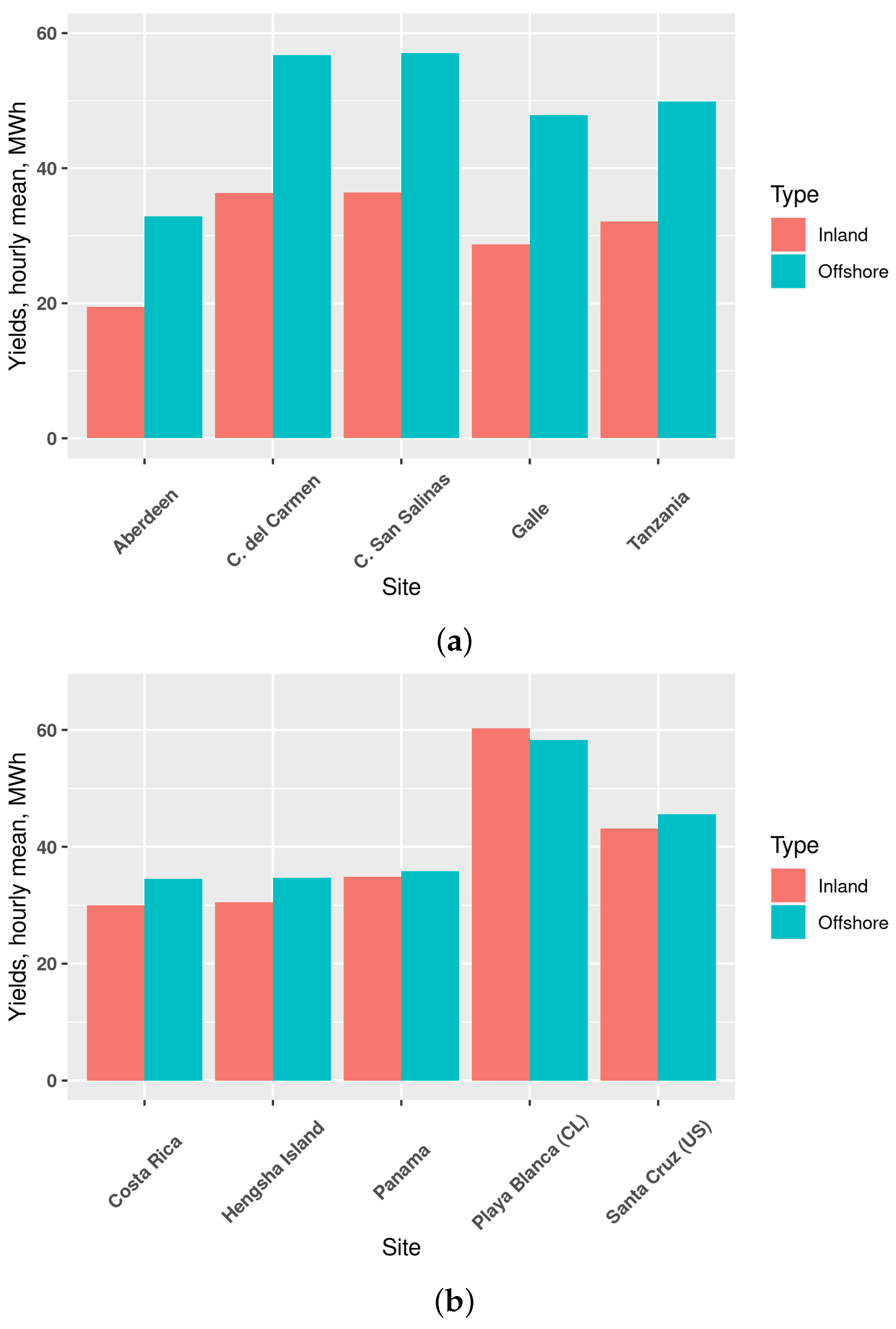
Across all 82 triplets of the sites in the final dataset, the offshore site on average generates 30% more electricity than the inland site. Depicted in Figure 6, essentially all sites witnessed a yield advantage ranging from 48% (Galle in Sri Lanka) to a minimum of approximately 1%. The two major exceptions were Playa Blanca in Antofagosta, Chile (coastal/port site located at −70.399° west, −23.668° south), where the offshore site generated 5% less yield, on an hourly basis, than the associated inland site. Likewise, the OFPV site in Santa Cruz, California (US) generated an average of 2% less yield than the associated LBPV.

The immediate explanation for this change compared to our previous work, where four out of twenty triplets had a “negative” yield advantage, is how our water cooling method, based on direct contact of the floaters with seawater, is modeled in this work in comparison to the previous work.

To justify this assertion, consider that the advantage in efficiency of the module is the main driver of the advantage in yield. This can in turn only be true if the cell temperatures/module temperatures are lower for the offshore sites than the inland sites. An intuitive explanation for this would be that the water surface, with which the floating panels are in thermal contact, would be consistently lower than the ambient air temperatures for the inland sites. Yet, our data do not bear this out, nor do we have evidence from our data that differences for wind speeds can drive the nearly uniform enhanced performance of the OFPV compared to the LBPV.

4.2. Resilience of the Regression Model

For ease of reference, we have placed a complete table showing the average hourly normalized advantage (in units of percentage) in Appendix B.

As explained, one of our aims will be to test the resilience of the multiple linear regression model developed in our previous work [7]. Specifically, we built a regression model that took into account the difference in insolation between the offshore and inland sites; the difference in total precipitation between the same two sites; and the difference in wind speeds between the offshore and inland sites.

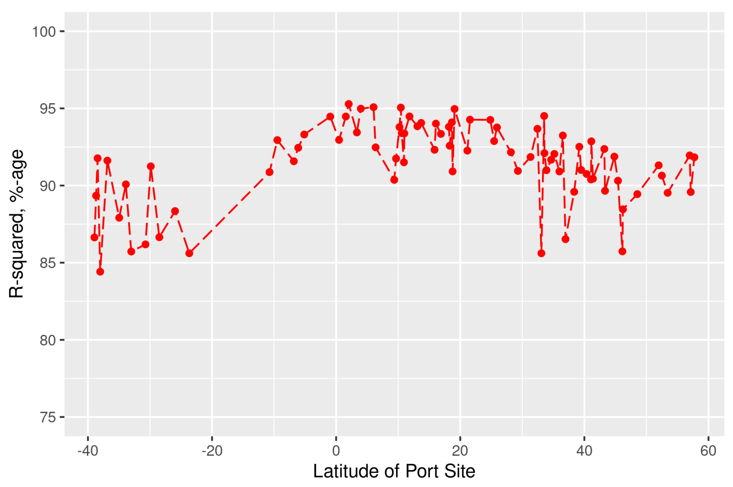
Unless otherwise stated, all of our results consider only hourly data where the insolation for each of the inland and offshore sites is ≥50 W/m². Note that this means that between 39% and 49% of all hours are taken into account, with the duration varying by geography and due to different insolation levels; on average, 44% of all the hours counted towards the calculations. As shown in Figure 7, the R-squared of this regression is relatively high and largely stable over the latitudes.

The major difference between the regression model we present in this paper and in our earlier work is that, in this paper, we use the difference in precipitation between the offshore and inland sites on an hourly basis instead of using only the precipitation for the inland site. Less drastically, in the previous work, we considered all hours where the insolations had a positive value (>0). In this paper, we consider only hours where the POA insolation (for both the offshore and inland sites) is ≥50 W/m².

We sought to determine the limits of this applicability by determining if the regression model’s parameters changed with variations in geography. In

Table 2. The limits (minimum and maximum) of the coefficients and the R-squared for our regression model findings.

	R-Squared	Intercept	delta_G_POA	delta_prec
Full dataset	(0.844, 0.953)	(−2.05, 0.62)	(0.55, 1.36)	(−0.03, 0.01)
Limited dataset	(0.844, 0.953)	(−2.05, 0.62)	(0.55, 1.36)	(−0.03, 0.01)
Extreme dataset	(0.857, 0.929)	(0.04, 0.14)	(0.92, 1.22)	(−0.02, 0.01)

, we show how the R-squared and also the coefficients for the independent variables in our regression model vary across our 82 sites. We divided this into three datasets: the full dataset with 82 sites; the “limited” with a total of 65 sites where the absolute value of the latitude is at most 40°; and the 17 “extreme” sites where the latitude is above 40°. Taken together, the similarity of these findings demonstrates that our regression is robust globally.

4.3. Cell Temperatures: Water Cooling of the OFPV

The main methodological innovation that this paper introduces compared to [7] is the new approach to modeling the operating temperature of the OFPV panels. We approached this question in two distinct ways, looking at all 82 triplets of sites and during the significant hours (i.e., whenever the insolation level is at or above 50 W/m²). For ease of comparison, we correlate these observations with the longitude and latitude of the corresponding port site.

In the first case, we compared the cell temperature of the offshore panels to the corresponding land-based panel (LBPV) for individual hours; we found that the cell temperature of the OFPV was lower than the LBPV cell temperature more than 75% of the time, although there was significant geographical variability across sites. In

Table 3. The five sites where OFPV cell temperatures are nearly always lower than the LBPV cell temperatures, expressed in relative number of occurrences.

Site	${\mathit{T}}_{\mathit{LBPV}}$ Lower [%]	${\mathit{T}}_{\mathit{WCM}}$ Lower [%]	LAT	LONG
Puerto Colombia	9	91	10.99	−74.96
Puerto La Cruz (VZ)	13	87	10.21	−64.63
Santa Cruz (US)	14	86	36.96	−122.02
Jeddah (SA)	14	86	21.57	39.11
Hengsha Island (CN)	14	86	31.32	121.85

, we show which sites are most likely to have similar OFPV and LBPV cell temperatures. In

Table 4. The five sites where OFPV cell temperatures are similar compared to the LBPV cell temperatures, expressed in relative number of occurrences.

Site	${\mathit{T}}_{\mathit{LBPV}}$ Lower [%]	${\mathit{T}}_{\mathit{WCM}}$ Lower [%]	LAT	LONG
Alanya (TR)	47	53	36.53	31.99
Girdle Ness/Aberdeen (UK)	47	53	57.14	−2.05
Beihai Port (CN)	40	60	45.42	141.68
Westport, OR (US)	38	62	46.13	−123.37
Cooper Reserve (NZ)	36	64	−36.87	174.74

, we list the five triplets of sites where the cell OFBV temperature is most likely to be always lower than the OFPV cell temperature.

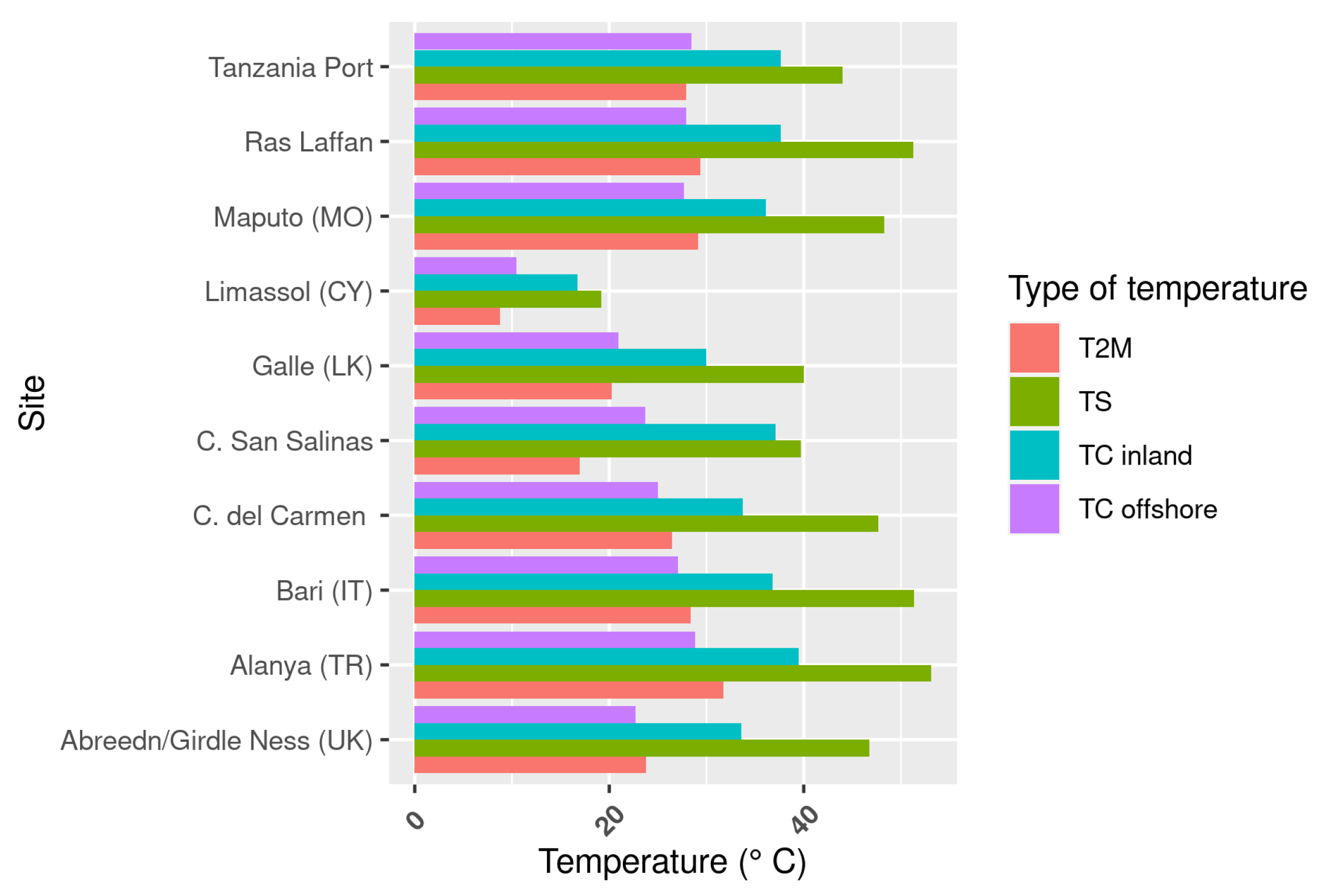
It should be noted that this could not easily be tied to a difference between ambient temperature and water surface temperature. Looking at all sites, and during hours with significant solar insolation, we found that the ambient air temperature inland was in general colder than the sea surface temperature during the same hour at the corresponding offshore site. This trend is highlighted in Figure 8, where we show the average values for the sea surface (TS), ambient (T2M), and cell temperatures for the 10 OFPV–LBPV pairs that have the highest normalized advantage.

Moreover, we found that, for 46% of our 82 triplet sites, sea surface temperature tends to be lower than the corresponding inland ambient temperature. Finally, we were not able to demonstrate a convincing correlation between the relative cell temperatures (i.e., the difference between the OFPV cell temperature and the LBPV cell temperature for any given hour) and the corresponding port site’s latitude ($R^2=26\%$).

Looking at our results, we can state first that the high likelihood of a positive advantage in yield from moving offshore that we predict elsewhere in this paper (the “offshore advantage”) is due in part to the fact that the cell temperatures are likely to be colder going offshore. Likewise, we can also demonstrate that this lower cell temperature for the offshore sites is due not necessarily to prevailing weather conditions (e.g., if the ambient temperature was simply much higher than the corresponding sea surface temperature) but results from the complex way that water cools floating panels, and which we sought to model with the WCM model. This second result will be extremely relevant for researchers attempting to predict the performance of OFPV but also invites further investigation of competing models of cell temperature. Of particular interest would be the impact of sub-surface currents and their impact on the siting of offshore FPV.

4.4. Classification of Yield Advantages vs. Geographical Classification

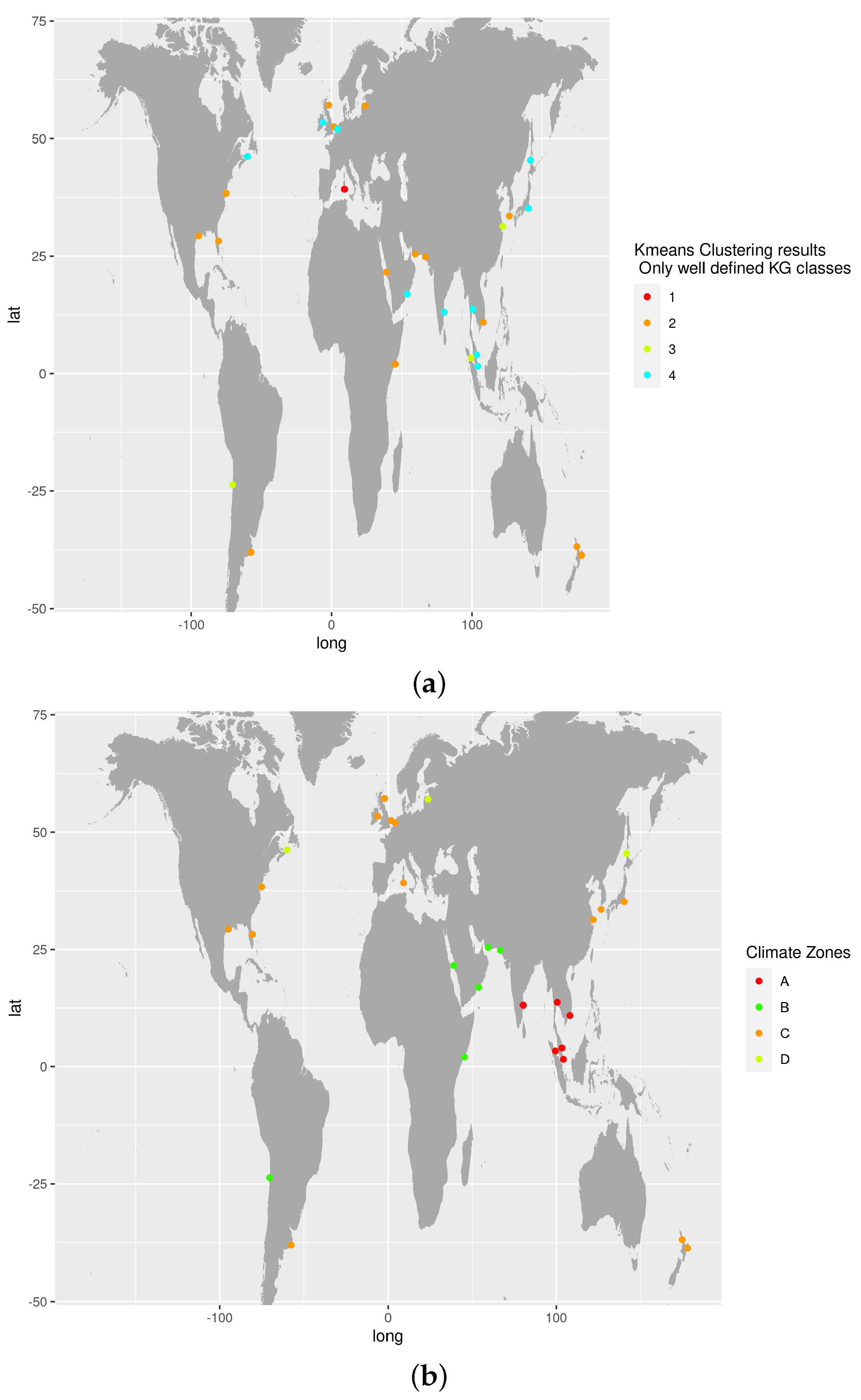
In this paper, we argue that relying on the KG climate classification system to determine the best sites globally for the deployment of offshore FPV would result in misleading conclusions. To provide evidence for this, we provide the following three sets of results using the k-means clustering algorithm.

4.4.1. k-Means Clustering with a Limited Subset

As stated in Section 2.2, the tool we use to determine the KG classification of the sites [19] also provides a quantification of the results. We thus limited ourselves to the sites where the KG classification has 100% certainty at first instance, giving us a total of 31 sites. We then focused only on the first level of the KG classification, the climate type. With this limited subset of 29 sites, we used the k-means clustering algorithm to sort the four represented climate types (“A”, “B”, “C”, and “D”). The results are presented in

Table 5. Results of k-means clustering to group the 29 sites, based on the averaged, normalized yield advantage, and climate zone, which is the first letter of the KG classification. All sites are clustered uniquely into one of four (4) distinct clusters.

Site	LAT	LON	Yield Advantage (%)	Climate Zone	Cluster
Aberdeen (UK)	57.14	−2.05	46.1	C	3
Caligari (IT)	39.19	9.16	40.4	C	1
Lowestoft (UK)	52.49	1.76	38.2	C	3
Cooper Reserve (NZ)	−36.87	174.74	36.9	C	3
Mogadishu	2.02	45.34	36.4	B	3
Jeju (RK)	33.52	126.54	36.3	C	3
Riga	56.97	23.86	36.2	D	3
Port of Rotterdam	51.98	4.13	33.4	C	4
Kaiti Beach (NZ)	−38.68	178.03	33.3	C	3
Howth (IE)	53.42	−6.14	33.0	C	4
Satellite Beach, FL (USA)	28.17	−80.59	32.9	C	3
Jedda (SA)	21.57	39.11	32.9	B	1
Phan Thiet (VT)	10.93	108.11	31.3	A	3
Mar del Plata (AG)	−38.02	−57.54	31.3	C	3
Jod (IR)	25.46	59.52	31.1	B	1
Galveston Island, TX (USA)	29.29	−94.79	30.1	C	3
Beihei (CN)	45.42	141.68	29.0	D	4
Ocean City, FL (US)	38.36	−75.08	28.2	C	3
Glace Bay, NS (CA)	46.21	−59.95	27.0	D	4
Kuantan (MY)	3.98	103.41	25.7	A	4
Bangkok (TH)	13.70	100.58	25.4	A	4
Katsuura (JP)	35.16	140.32	25.0	C	4
Karachi (PK)	24.84	66.81	24.5	B	3
Chennai Port (IN)	13.10	80.30	22.0	A	4
Mughsail Beach (OM)	16.88	53.79	20.0	B	4
Bandar Penawar (MY)	1.56	104.23	19.8	A	4
Kwala Tanjung (MY)	3.35	99.45	15.8	A	2
Hengsha Island (CN)	31.32	121.85	13.7	C	2
Antofagasta (CL)	−23.67	−70.40	−5.5	B	2

.

The same data are repeated in more compact form in

Table 6. The k-means algorithm does not always place sites with similar KG climate classification in the same eventual cluster.

Cluster	Climate Zone within Cluster
Cluster 1	A B B C C C C C C C C C D
Cluster 2	B B C
Cluster 3	A A A A B C C C D D
Cluster 4	A B C

, with the clusters (found by running the k-means algorithm against the yield advantage data) shown together with the KG climate classifications found in each cluster.

This mismatch between the clustering results and the climate zones is illustrated in Figure 9 below.

4.4.2. k-Means Clustering with Specific Climate Types

As illustrated in Table 6, we demonstrate that the KG climate classification system can predict the outcomes of the yield advantage. This can be seen by the way in which our unsupervised clustering algorithm, when classifying sites by the yield advantage, does not group even sites within the same basic climate zone (“A”, “B”, “C”, or “D” for tropical, arid, temperate, and continental) together.

Nonetheless, and as is shown throughout this paper, there is a clear geographic dependence on the performance of the FPV sites, but the amount of geographic and meteorological data one needs to make informed predictions about PV performance is much more detailed than is captured by the KG system.

4.5. Economic Comparisons: LCOE in Two Pairs of Triplets

Aside from the differences in PV yield and performance, there are economic considerations that could determine the appropriateness of a given site for the deployment of offshore FPV. In this section, we focus on how differences in economic conditions between countries that are otherwise comparable would lead to differences in the cost of solar energy for offshore solar farms.

We focused on two pairs of sites as follows.

1.

The first pair was the Miyazaki Port site in Miyazaki, Japan, compared against the Hengsha Island site in China. Both of these sites have a KG climate classification of “Cfa”.

2.

The second pair was the Port of Rotterdam offshore site, which we compared with the Girdle Ness site in Aberdeen in the UK, both with a KG climate classification of “Cfb”.

In all four cases, we have 100% certainty for the KG classification. Our results are presented in

Table 7. The variation in LCOE across sites that are in some way comparable helps to illustrate how geography and economic factors interact in this study.

	Rotterdam	Aberdeen	Miyazaki	Hengsha
Offshore yield advantage (%)	33.1	46.1	25.1	13.7
Offshore CAPEX, $/kW	2204	1829	3652	1355
Offshore LCOE, $/MWh	49.61	46.17	67.83	30.30
Inland CAPEX, $/kW	1022	848	1693	628
Inland LCOE, $/MWh	27.80	32.41	34.33	13.16
Offshore CAPFAC	15%	14%	18%	15%
Inland CAPFAC	10%	7%	13%	13%

.

While based on very limited data, we are able to argue how differences not only in geography but also in economic conditions can create pronounced differences in pairs of sites that seem otherwise very comparable. This is held up by, for example, large differences in the upfront installation costs between a site in China and a site in Japan. To consolidate the overall differences, we make use of the widely known metric of the capacity factor, CF:

$$\mathrm{CF}=\frac{{\sum }_{\mathrm{h}=1}^{{\mathrm{n}}_{\mathrm{hours}}}{\mathrm{P}}_{\mathrm{hourly}}}{{\mathrm{n}}_{\mathrm{hours}}\ast \mathrm{Capacity}}$$

(9)

where ${\mathrm{n}}_{\mathrm{hours}}$ is the number of hours over which we are summing the data and ${\mathrm{P}}_{\mathrm{hours}}$ is the hourly generation of electricity (the yield). Typically, ${\mathrm{n}}_{\mathrm{hours}}$ is taken to be the number of hours in a year, in our case covering the 10 years of data of 87,672 h. In short, the capacity factor, which can be applied to any type of electricity generation technology, provides us an easy way to compare how effective a specific site is relatively. Applied to our pairs of sites, the differences in capacity factors, which are themselves determined by differences in meteorology, can lead to stark contrasts in the LCOE, as illustrated in Table 7.

Our approach to calculating LCOEs has so far been preliminary; however, it seems that we can state with moderate certainty that clearer skies on offshore sites—leading to relatively higher offshore capacity factors—would be a major driving factor in determining the economic viability of an offshore solar PV installation. The clearest example of this is how the LCOE from OFPV in Aberdeen is potentially lower than the LCOE from OFPV in Rotterdam despite very similar offshore capacity factors. Meanwhile, the much cloudier conditions over the Aberdeen site mean that the situation is reversed for LBPV, with Rotterdam being able to produce solar PV electricity cheaper than Aberdeen.

4.6. Brief Summary of the Results

In summary, we can summarize the main findings of our paper as follows:

1.

Placing PV panels offshore is likely to lead to significant improvements in the performance of those panels located offshore when compared to a land-based panel equidistant from a coastal port site. We considered multiple metrics, including cell temperature, efficiency of the modules, and yields.

2.

We can show that this improvement, or “offshore advantage”, is a direct result of the method of water cooling by placing the panels in thermal contact with water bodies. It is not a result, for example, of any difference in temperature between the sea surface temperatures and ambient air temperatures inland, and, in any case, we found that sea surfaces were often consistently higher than the ambient air temperatures inland.

3.

We found that there was a clear and detectable relationship between the extent of that “offshore advantage” and the geography of a site. This relationship did not extend, however, to the KG climate classification system, which we find to have a limited impact on determining either whether a given site is a good contender for conventional solar PV installations or for the deployment of OFPV.

4.

We found that, beyond geographic and meteorological considerations, economic development can help to determine whether or not a given site is a good host for OFPV.

5. Conclusions

We set out to determine if there were general rules to determine which sites across the globe would provide the greatest feasible advantage to deploying offshore floating PV modules placed on top of pontoons. We accomplished this by modeling the output for a large number (82) of OFPV locations, roughly ∼55 km from the shore, and scattered around the globe. We then compared the hour-by-hour performance of each individual offshore location with the output from a land-based PV system (LBPV) at a distance of ∼110 km inland.

A number of the important conclusions of this paper stand out. Firstly, we were able to demonstrate that there is a meaningful correlation between geography and the enhanced performance of offshore FPV compared to land-based PV systems. We were able to achieve this using a greatly expanded dataset (n = 82) compared to our earlier work. Further, we also demonstrated that the projected offshore advantage is almost certainly tied to the method of water cooling of the OFPV, specifically assuming that the OFPV panels are in thermal contact with the seawater.

In addition, our data show that the insolation levels tend to be higher for offshore sites compared to inland sites, driven by higher clear sky indices for a given offshore site compared to its corresponding inland site. Nonetheless, this increased insolation is not as much of an explanatory factor for the differences in yield.

While our WCM for the cooling of the offshore panels could be enhanced in the future, our results show that any future modeling work related to the performance of offshore PV should not ignore the impact of water cooling methods. It goes without saying that the floating structure is imperative in this.

In terms of geographic classifications, our results show that we cannot take the Köppen-Geiger climate classification system as a proxy to predict where (and where not) to deploy offshore PV panels. In contrast, we can show that there are strong correlations between the offshore advantage and geography and meteorology, and particularly within latitudes ≥40 (north and south), hence outside the sunbelt regions around the equator.

Finally, we explored how economic factors, specifically the differences in capital costs to build utility-scale solar, could lead to distinct differences in cost differentials for OFPV when pairs of sites share a complete KG climate classification.

Further Research and Future Steps

We provide below a non-exhaustive list of possible projects to build on the present effort, in increasing order of difficulty and complexity:

• Understanding the impact of orientation of panels and cell technology. Optimization of tilt and orientation (e.g., using bifacial panels) and/or technology (e.g., non-silicon panels or heterojunction cells) would impact the overall project cost as well as the yields. It should be possible to determine optimal combinations of orientations with cell technology.
• Hybrid offshore wind-solar systems. Offshore wind power, although limited to a few locations, is certainly more well developed than OFPV. Questions that remain to be explored include the degree of synergy between OFPV and offshore wind, the impacts on total system costs, and the relationship between geography and offshore hybrid systems. Researchers may also wish to consider the needed upgrades to existing offshore wind electrical infrastructure to make OFPV/offshore wind hybrids possible.
• Further studies on the economic aspects of OFPV. Given the dearth of comparable high-quality economic data for a wide range of regions, it will be difficult to come to a reliable conclusion on which sites are economically feasible as locations for the siting of OFPV.