Modeled and Measured Operating Temperatures of Floating PV Modules: A Comparison

Abstract

The power output of a photovoltaic system is dependent on the operating temperature of the solar cells. For floating PV (FPV), increased wind speeds can result in increased yield due to lowered operating temperatures, which has long been stated as a key advantage for FPV. So far, this effect has not been included in commercial software packages for yield estimation. Typically, only standard settings are provided, taking into account the mounting type (PVsyst) or mounting and module type (Sandia). This may result in an underestimation of the yield, and consequently, the estimated Levelized Cost of Electricity (LCOE) of the FPV project. In this study, a linkage between recorded module temperatures from FPV systems located in The Netherlands and Sri Lanka and the prevalent models employed within PVsyst and Sandia software for estimating module temperatures are established. Our findings reveal that the models within PVsyst and Sandia tend to overestimate module temperatures by 2.4% and 3%, respectively, for each 1 m/s increment in wind speed. We present two methods for determining the single heat loss coefficient, or U-value, tailored to specific sites accounting for local wind conditions. The first method computes the U-value based on the average monthly wind speed, whereas the second employs the irradiance-weighted average monthly wind speed. The latter method can be advantageous for locations characterized by significant fluctuations in wind speeds between night and day. Through a statistical residual analysis comparing measured and modeled module temperatures, we demonstrate that our proposed methods offer a more accurate representation of module temperature compared to the PVsyst and Sandia models when default settings are used. When we subsequently compute the specific yield using both measured and modeled temperatures, we observe that the approach using irradiance-weighted average wind speed shows a higher yield of up to 2% compared to the traditional methods.

1. Introduction

The aspect of lower operating temperatures for floating PV (FPV) systems has, for a long time, been stated as one of the key advantages of FPV, as the operating efficiency is expected to be higher. The operating temperature of a photovoltaic module is determined by several factors such as: incident solar radiation, ambient temperature, wind speed, wind direction, properties of the cell and module materials, and mounting structure. Both radiative and convective heat transfer will take place and affect the module temperature. Numerous models have been proposed for the estimation of the module temperature, and a comprehensive overview is given by Skoplaki et al. [1]. As FPV systems are in close proximity to the water, other factors may also impact the operating temperature. In the first comparative study on pilot FPV systems, Liu et al. showed that the level of reduced operating temperature, compared to a roof top system, was dependent on the system design and the level of water footprint created by the floater structure [2]. For some system designs directly in thermal contact with water, the level of cooling has also been shown to be dominated by the water temperature [3,4]. A range of studies have investigated the characteristics of operating temperature for FPV, such as Kamuyu et al., who reported on decreased operating temperatures and proposed a temperature model using multivariable linear regression [5]. The same multivariable linear regression approach was applied in a study by Hayibo et al. [6]. More complex physical models incorporating the radiative heat transfer between the water surface and the module have been proposed, in addition to also considering the changes in humidity levels and the effect of seawater splashing and its evaporation on the modules [4,6,7].

For energy yield assessment (EYA) in commercial software, simplified temperature models are often used, and these are described in more detail in Section 2. The large variety of models applied in the various scientific reports mentioned above proves that it is challenging to directly compare the empirical constants reported for different FPV systems and to directly apply the research to the existing methodology used by the PV industry. The primary goal of this paper is to establish a connection between recorded module temperatures of FPV systems and prevailing models used within commercial software used for EYA, such as PVsyst and Sandia software packages (e.g., Pvlib, versioin 0.10.1) for the purpose of estimating module temperatures. We compare the measured operating temperatures with both the Sandia and the PVsyst temperature model. However, only the PVsyst model is applied when computing the empirical constants at each site, as these will apply for the Faiman model; hence, it can be directly used when applying Pvlib. In addition, the paper introduces a novel methodology that accurately integrates the advantages resulting from increased wind conditions for modeling the temperature of FPV modules within the respective software. Lastly, a comprehensive examination of these temperature models was conducted to evaluate their influence on the electrical yield.

2. Materials and Methods

2.1. Operating Temperature of PV Modules

The most commonly used model for estimating the operating temperature of PV modules, which also is the recommended model given in IEC61853-2 [8], is the model based on heat balance proposed by Faiman [9]:

$$T_{mod}=T_{amb}+\frac{G}{{U^{\prime }}_0+{U^{\prime }}_1\times v}$$

(1)

where U′₀ = U₀/(α – η) and U′₁ = U₁/(α – η), and where T_amb (°C) is the ambient temperature, T_mod (°C) is the module temperature, α is the absorbed fraction of the incident irradiance (set to 0.9), G (W/m²) is the incident irradiance on the plane of the module, η is the electrical efficiency of the module, v (m/s) is the wind speed, measured at a height of 3–5 m above ground, and U₀ and U₁ are wind independent and dependent heat loss coefficients (W/m²K), respectively. For land-based PV (LPV) systems, the values of the heat loss coefficients and their correlation with various meteorological parameters have been thoroughly studied [10,11,12], but the most appropriate values of U₀ and U₁ for the various types of mounting structures are still debated. This is not surprising as U₀ and U₁ will depend on module characteristics, outdoor conditions, and mounting, and hence, a significant spread in best-fit values for different systems is expected. In the standard, IEC61853-2, it is recommended to find the appropriate values for each site [8]. It is also worth mentioning that another temperature model, derived from the heat balance model from Faiman [9], is applied in the most commonly used energy yield assessment (EYA) tool, PVsyst:

$$T_{cell}=T_{amb}+\frac{\alpha \left(G\right)\left(1-{\eta }_{PV}\right)}{U_c+U_v\left({\nu }_{10m}\right)}$$

(2)

where T_cell (°C) is the cell temperature, U_c is the radiative heat loss coefficient (W/m²K), U_v is the convective heat loss coefficient (W/m³Ks), and v_10m is the wind speed at a height of 10 m (m/s).

Another model for estimating the operating temperature is the Sandia model. This is a heat transfer model with empirically determined parameters developed by King et al. [13]:

$$T_m=G{e}^{\left(a+b{w}_s\right)}+T_{amb}$$

(3)

where a is an empirically determined coefficient establishing the upper limit for module temperature at low wind speed and high solar irradiance, b is an empirically determined coefficient establishing the rate at which the module temperature drops as wind speed increases, and v is the wind speed measured at a height of 10 m. When comparing the two different models, it is important to note that the temperature model in PVsyst provides the cell temperature, whereas the Sandia model provides the module temperature. The two can be related through [13]:

$$T_{cell}=T_m+\frac{G}{G_0}\mathsf{\Delta }T$$

(4)

where G₀ is the reference irradiance of 1000 W/m² and ΔT is the temperature difference between the cell and back-of-module temperature at an irradiance of 1000 W/m². In this work, a ΔT of 3 °C is used, as suggested for open rack modules by King et al. [13]

2.2. Overview of Heat Loss Coefficients

Over the years, different studies have addressed the topic of heat loss coefficients (U_0′ and U_1′, U_c and U_v) and empirical values for parameters a and b, as utilized in the Sandia model for ground-mounted, open-rack solar panel systems. Some of these values are documented in

Table 1. Overview of several heat loss coefficient and empirically determined values for a and b. A distinction has been made between land-based (LPV) and floating PV (FPV).

System	U0′ [W/Km2]	U1′ [Ws/Km3]	Uc [W/m2K]	Uv [W/m3Ks]	a [-]	b [-]	Reference
LPV (open structure, Negeve desert)	26.86	6.11			−3.38	−0.13	Köhl et al., 2011 [12]
LPV (closed structure, Alps)	28.04	7.77			−3.55	−0.12	Köhl et al., 2011 [12]
LPV (Open rack, glass-cell-glass)					−3.47	−0.0594	King et al., 2004 [13]
LPV (Open rack, glass-cell-polymer)					−3.56	−0.0750	King et al., 2004 [13]
LPV (Open rack, wind independent)			29	0			PVsyst, 1996 [15]
LPV (Fully insulated backside, wind independent)			15	0			PVsyst, 1996 [15]
LPV (Open rack, with wind dependency)			25	1.2			PVsyst, 1996 [5]
FPV (open structure, The Netherlands)			24.4	6.5			Dörenkämper et al., 2021 [14]
FPV (closed structure, The Netherlands)			25.2	3.7			Dörenkämper et al., 2021 [14]
LPV (open structure, The Netherlands)			18.6	4.4			Dörenkämper et al., 2021 [14]

. Furthermore, some default settings for the PVsyst model package can be found, which were validated by several PV systems in Switzerland in 1996. The variability in all of these values can be attributed to factors such as location-specific influences, disparities in wind measurement heights, and local variations affecting wind patterns. In the case of FPV systems, variations in heat loss coefficients have been observed to be substantial not only due to design-related factors but also geographical dependencies [14]. Systems featuring a significant water surface area, densely arranged modules, and limited air circulation behind the modules tend to exhibit lower heat loss coefficients when compared to systems with a smaller water surface area and ample air circulation behind the modules.

To illustrate the dependency of operating temperature on the respective empirical constants, such as a and b for the Sandia model and the heat loss coefficients used in the PVsyst model, a contour plot is presented in Figure 1. This plot illustrates the modeled module temperature at an ambient temperature of 20 °C and an irradiance of 800 W/m², while considering various combinations of a and b values in addition to U_v and U_c values.

2.3. Software Packages

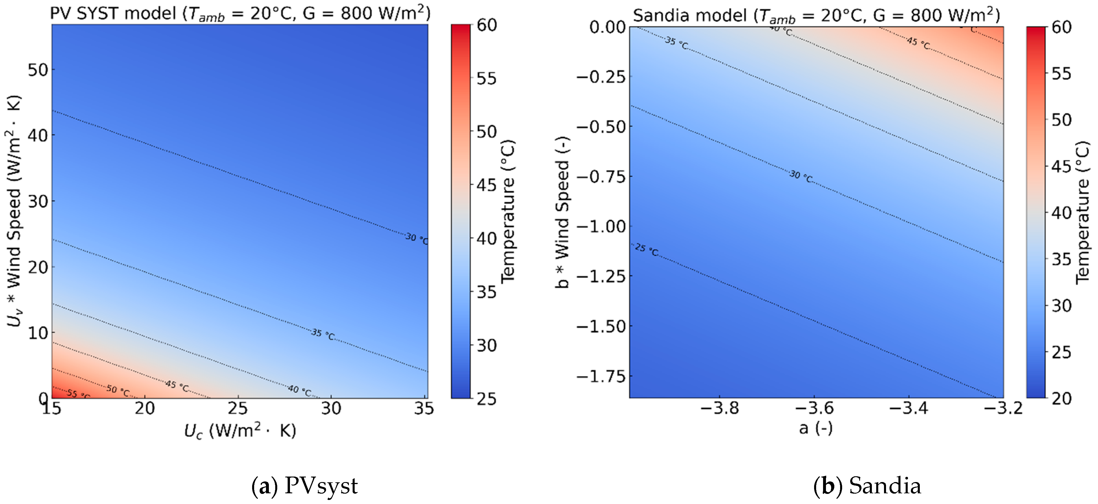
PVsyst and Pvlib are two software packages that are widely used to predict the electrical yield of a PV system at a certain location. Although PVsyst can currently be claimed to be the most commonly used software for the industry, Pvlib often forms the basis for work within research. Within this work, we compare measured PV module temperatures with modeled PV module temperatures obtained when the default settings within PVsyst and Pvlib are applied by making use of their equations within Python. The two software packages are described below. It should be mentioned that a wide variety of software packages for this purpose exist. However, the same temperature models are often applied within the different packages; hence, the results of this work are also transferable to other commercially available tools.

2.3.1. PVsyst

PVsyst is a software package designed for solar energy applications. It assists professionals in designing, simulating, and analyzing PV systems. By inputting parameters like location, module specifications, and system components, users can optimize PV module arrangement. The software estimates energy yield based on weather data, system setup, and technology specifications, providing daily and monthly production estimates. Additionally, PVsyst performs financial analysis by considering costs, incentives, financing, maintenance, and operational expenses. The temperature model in PVsyst is based on the Faiman temperature model. There are default settings for U_c and U_v, as described in Table 1. Users have the flexibility to modify these settings. Typically, meteorological data is imported from Meteonorm. However, other sources are also available, as well as the possibility to import custom meteorological datasets. It should be noted that based on the current recommendations in PVsyst, it is common to set U_v = 0 W/m³Ks, assuming a constant wind speed on site.

2.3.2. Pvlib

Pvlib (Photovoltaic Library) is an open-source (Python and Matlab) library used for modeling and simulating solar energy systems [16]. Developed in 2012 at Sandia National Laboratories as part of the PV Performance Modeling Collaborative (PVPMC), it offers various functionalities, including solar position calculations, clear sky irradiance modeling, and PV system performance modeling based on mathematical models and empirical data. Pvlib is widely utilized by researchers, engineers, and developers in the solar energy field to assess system performance, optimize design, and analyze different scenarios. Its modular structure allows users to customize and combine components for specific applications, making it a valuable resource for solar energy simulations and analyses. Pvlib offers a range of different temperature models, including the Sandia model and the Faiman model, both allowing to set a value for the empirical constants.

2.4. PV Systems

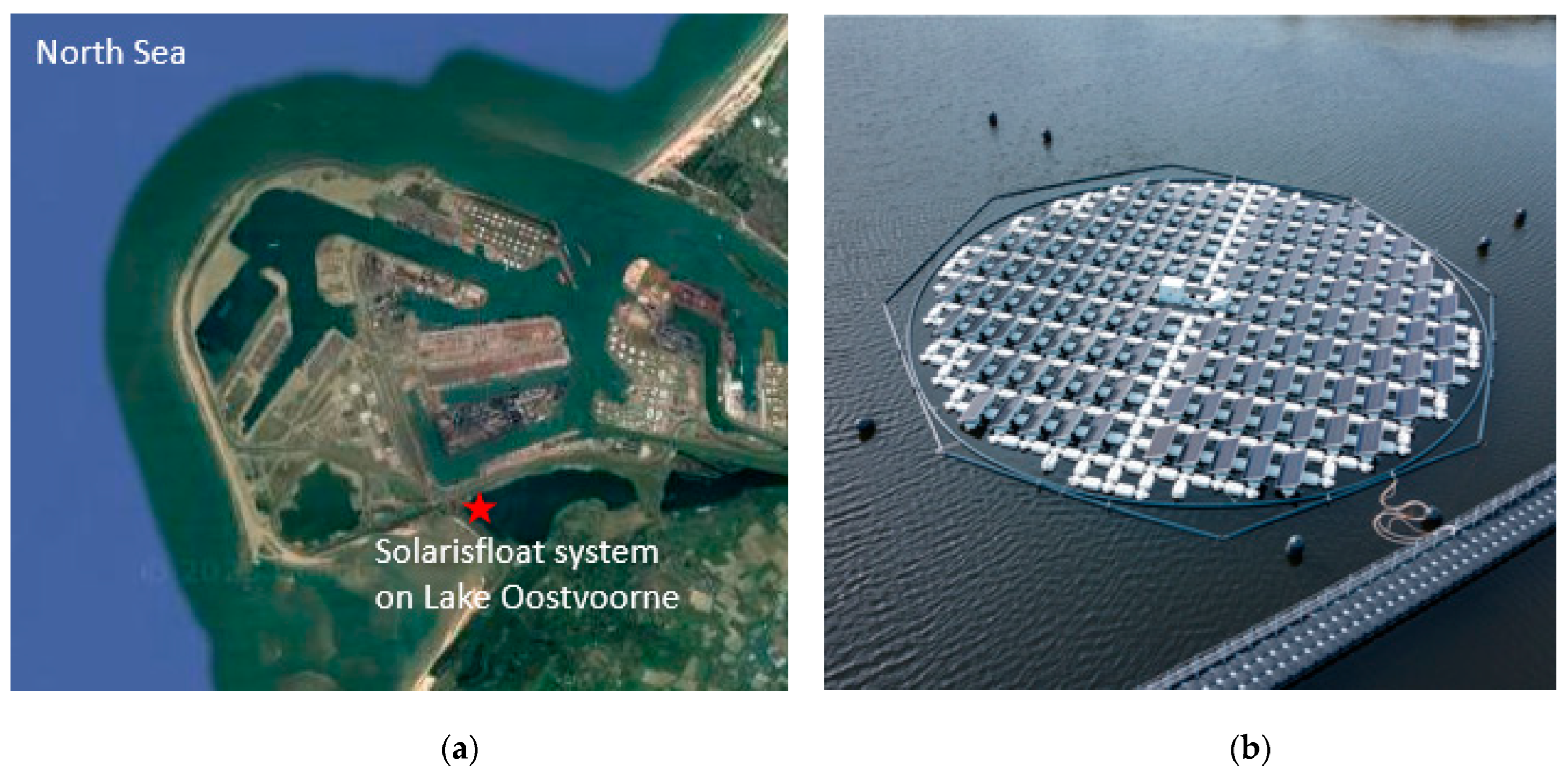
2.4.1. Solarisfloat in The Netherlands

The PV system, developed by the Portuguese company Solarisfloat, has been deployed on Lake Oostvoorne. This lake is situated in the west of The Netherlands, near the North Sea. It has a surface area of around 270 hectares. In Figure 2, a satellite image of this lake can be found together with an aerial view of the Solarisfloat system.

The Solarisfloat system is a ~50 kWp floating azimuthal tracking PV system. It utilizes mono-crystalline PERC modules, each rated at 390 Wp. The system consists of 128 PV panels tilted at 25° and divided into 8 strings. These strings are connected to a land-based inverter (SMA Sunny Tripower STP 50-40). Each module is mounted on an aluminum frame that is connected to several floaters, providing buoyancy. The PV panels are oriented towards a single side, allowing ample airflow to cool the rear side of the panels. The system can rotate around its center using several propellers, allowing azimuthal tracking of the sun. Pt100 temperature sensors, with an accuracy of ±0.15 °C (0 °C) and ±0.35 °C (100 °C), are installed on the rear side of selected panels, and an average temperature value from these sensors has been used for further analysis. The plane-of-array (POA) irradiance is measured by a EKO MS-802 pyranometer (zero offset < 3%) mounted above a module on the rotating system. Ambient temperature and wind speeds were recorded by a WT600 Lufft weather station (accuracy temperature measurements ±0.2 °C, accuracy wind speed measurements ±3%) positioned 3 m above ground level. The weather station is located approximately 80 m north of the PV system on the shore. Measurements were recorded between January and October 2021 and from September until December 2022, with a time interval of 1 min.

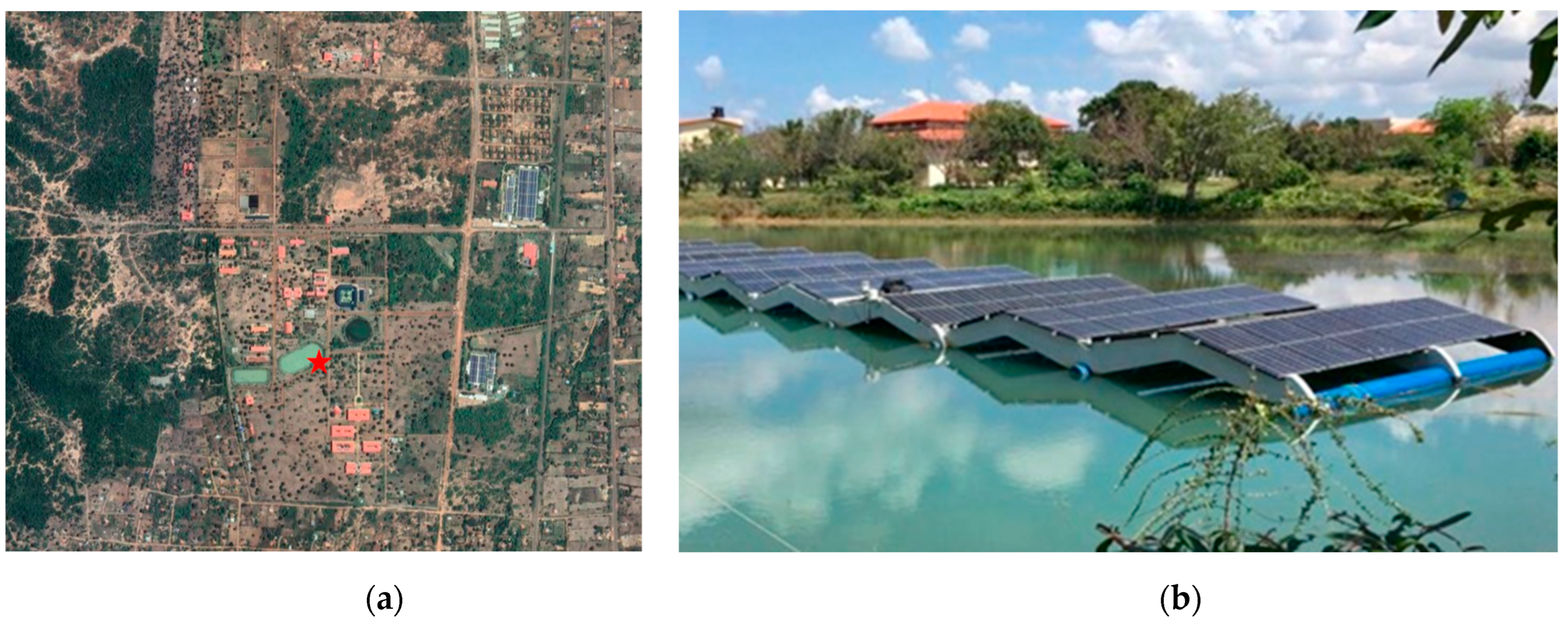
2.4.2. Current Solar in Sri Lanka

The PV system developed by the Norwegian company Current Solar AS was deployed on a small and calm water body in Kilinochichi, Sri Lanka, and is shown in Figure 3. The rated installed capacity is 44 kW, and the system consists of composite beams mounted on high-density polyethylene pipes to provide buoyancy. The PV modules are mounted in an east-west orientation with a 15° tilt and consist of both mono-crystalline REC Solar N-Peak 315 Wp and multi-crystalline REC Solar TwinPeak 295 Wp modules. The strings are connected to a land-based 50 kW SMA inverter. The POA irradiance in each direction is measured by Kipp&Zonen RT1 Smart Rooftop Monitoring Systems (accuracy of ±3%), which also provides a back-of-module temperature (accuracy of ±1 °C. Ambient temperature and wind speeds were recorded by a Campbell scientific METSENS500 (Campbell scientific, Logan, UT, USA) compact weather sensor located on top of the FPV system, at the same height as the top of the module (accuracy of ±0.3 °C for ambient temperature and ±3% for wind speed). Measurements were recorded between September 2021 and September 2022, with a time interval of 10 min.

2.5. Data Handling

In this work, measured wind speed, air temperature, and POA irradiance are used to model the module temperatures for the two mentioned systems. To ensure that factors such as missing values, unphysical measurement data, and stale sensor readings do not affect the reported outcome, the raw data was filtered before proceeding with the calculations. For the calculation of the heat loss coefficients, wind speed and temperature measurements outside reasonable limits were removed, and only times with irradiance above 250 W/m² were included. To reduce the impact of time periods where the system is far from equilibrium due to rapidly changing irradiance, the data was aggregated to time periods of 10 min. The module temperatures were modeled within Python by making use of the models as used within the software package PVsyst and Pvlib. For the PVsyst model, a default U-value of 29 W/m²K was used. For the Sandia model, empirical constants of a = −3.56 and b = −0.075 were used, together with a wind speed of 1 m/s.

2.6. Wind Speed Height

The wind speed can vary greatly depending on the height compared to the ground and the roughness of the landscape. Within the models of PVsyst and Sandia, a standard wind speed height of 10 m is used, most likely as this is the typical wind speed height when using wind speeds from available metrological datasets. To correct for our wind speed measurements, which were measured at a height of 3 m (Oostvoorne) and 1.5 m (Sri Lanka), the following equation was used [17]:

$$V_{10}=V_{meas}\left(\frac{\ln \left(\frac{10}{z_0}\right)}{\ln \left(\frac{z_{meas}}{z_0}\right)}\right)$$

(5)

where V₁₀ represents the modeled wind speed at a height of 10 m (m/s). V_meas is the measured wind speed (m/s), z₀ stands for the roughness length of the surface (m), and z_meas denotes the height at which the wind speed is measured (m). The roughness length varies depending on the type of surface and the landscape on which the measurements are performed. Our measurements are either performed on land, but nearby open water, or in the middle of a small pond. Therefore, we used a value of 0.03 m, which is a standard roughness for grassland or open fields without obstacles.

3. Results

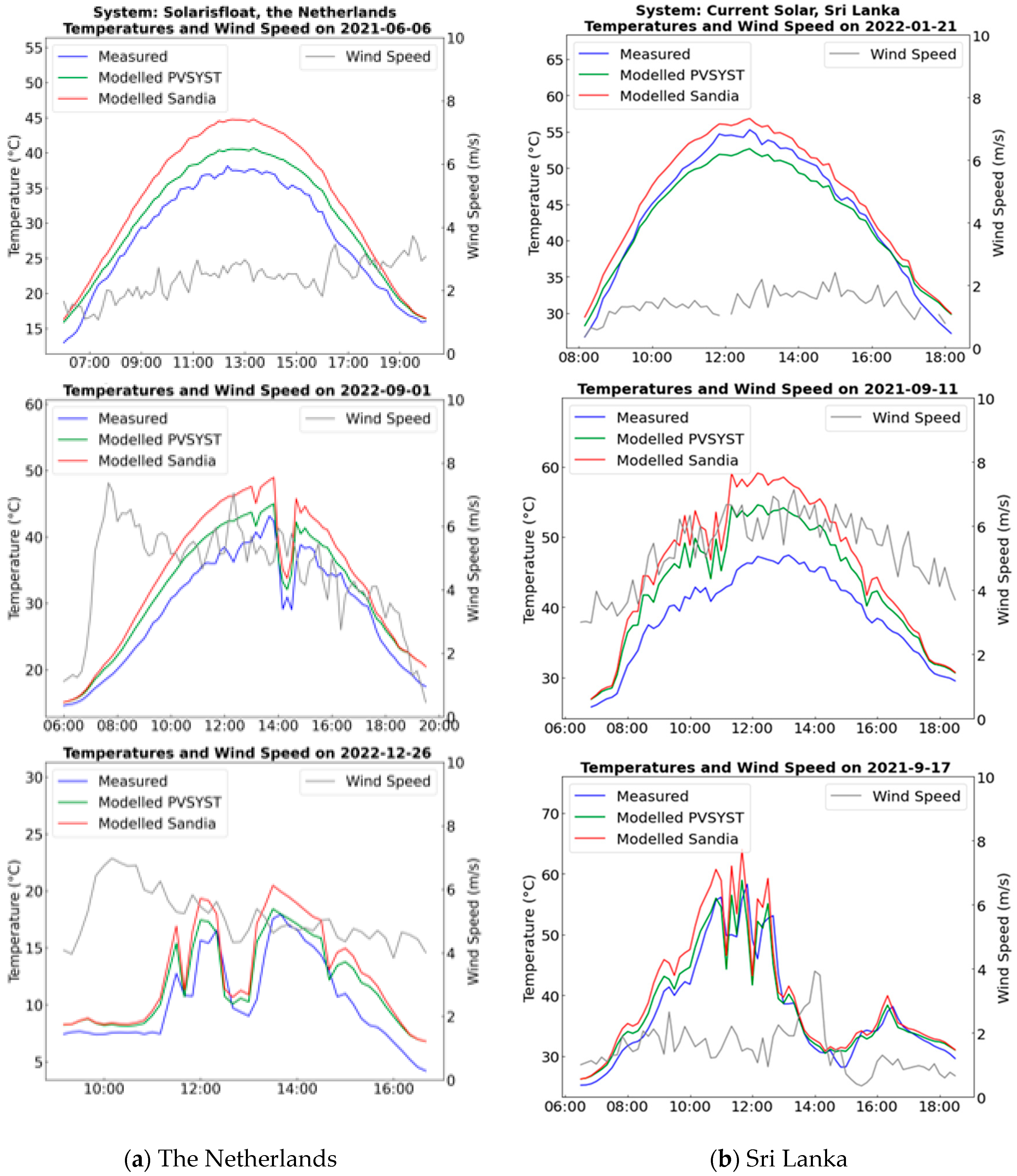
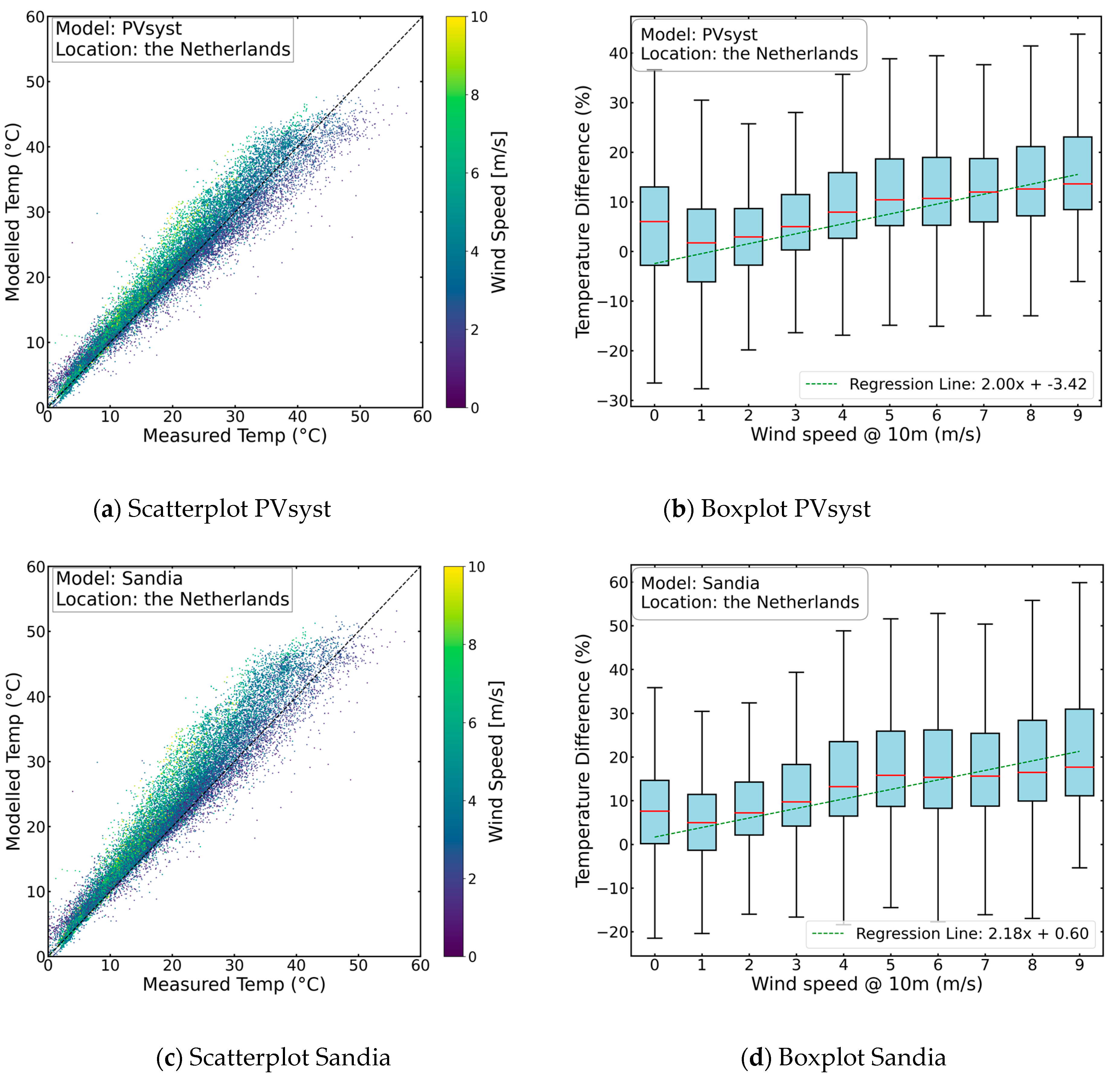
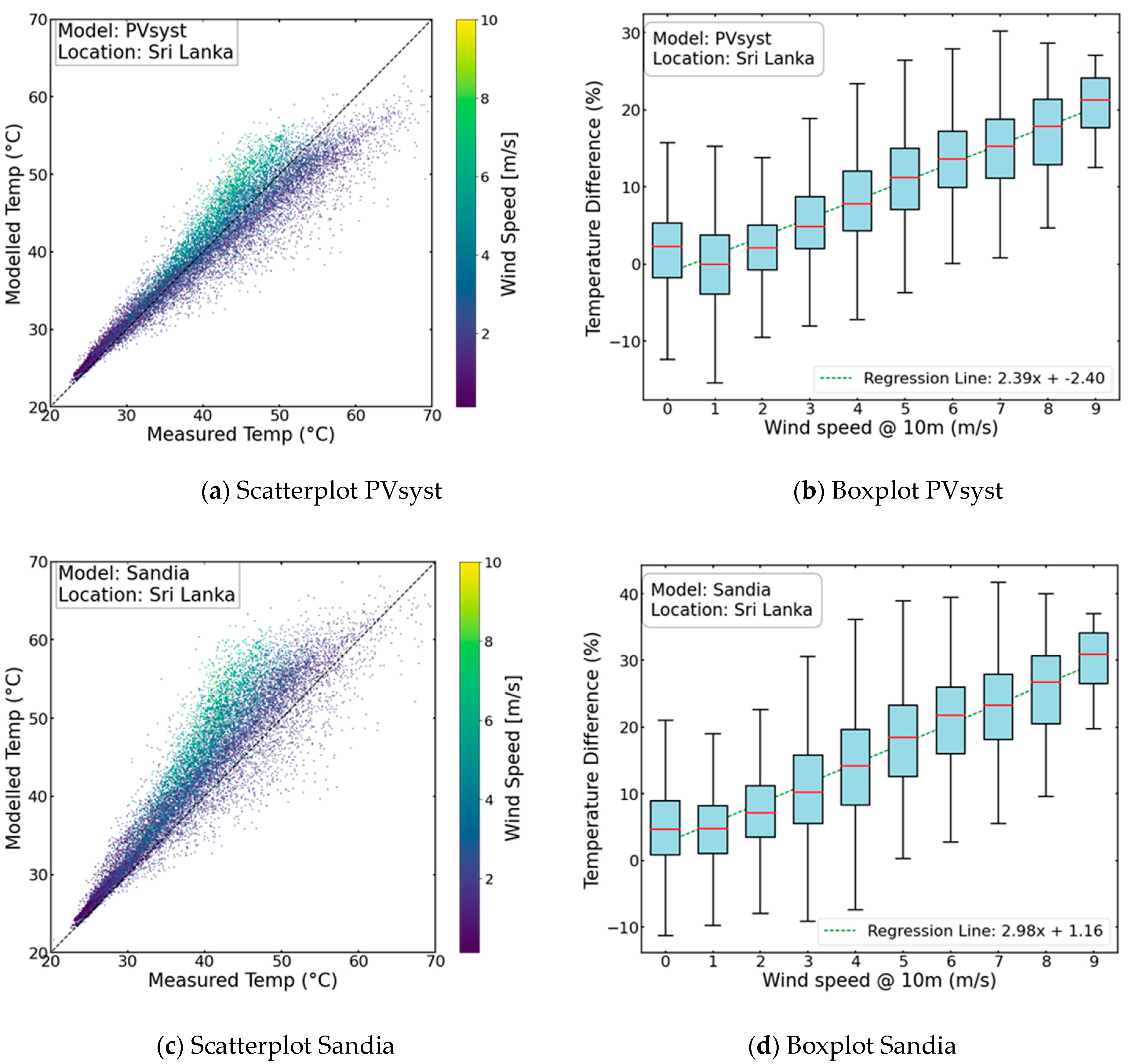
3.1. Direct Comparison of Measured Temperature Data with Modeled Data

In Figure 4, a direct comparison is presented between measured and modeled temperatures for both systems on a few representative days. The left side of the figure displays temperatures from the Solarisfloat system along with the measured wind speed data. Specifically, the 6 June 2021 was characterized by sunny weather and relatively low wind speeds. On the 1 September 2022, it was sunny with medium wind speeds, and the 26 December 2022 experienced partly cloudy conditions with moderate wind speeds. Observations reveal that, on all three days, the modeled module temperatures were higher compared to the measured temperatures. Notably, on the 6 June 2021, around solar noon, the difference reached a maximum of approximately 8 °C between the measured and modeled data using the Sandia model. Even under low wind speed conditions, significant differences were observed. The right side of the figure displays temperatures from the Current Solar system located in Sri Lanka. The 21 January 2022 was characterized by sunny weather and low wind speeds, and under these conditions, both models represent the measured temperatures well, although there is a slight overestimation for the Sandia model, whereas the PVsyst model underestimates the module temperature. However, for a day with relatively sunny weather but higher wind speeds, such as on the 11 September 2021, the modeled temperatures were higher than what was measured, with the largest difference at 15 °C around solar noon between the measured and modeled data using the Sandia model. On the 17 September 2021, the conditions were overcast and medium-to-lower wind speeds. Also, here, the modeled temperatures were higher, but to a lower degree than for days with higher wind speeds and higher irradiance.

Figure 5 and Figure 6 present an analysis of the temperature difference between the measured and modeled data encompassing the entire datasets. On the left side of the scatterplots, we depict the modeled data as a function of the measured data, with the dotted line serving as a reference for equality, representing instances where the modeled temperature matches the measured temperature. The color bar in the figure provides additional insight by indicating the measured wind speed at a height of 10 m for each data point. Notably, a consistent trend emerges, revealing that the modeled temperature generally exceeds the corresponding measured temperature, and this discrepancy intensifies with increasing wind speed. This pattern holds true for both the Sandia and PVsyst models. To delve deeper into the nature of this discrepancy, we conducted an analysis by computing the temperature difference, where the modeled minus the measured temperature is calculated as a percentage of the measured temperature and subsequently binning this difference based on wind speed intervals of 1 m/s. The results of this examination are portrayed on the right side of the figure, alongside the outcomes of a linear regression conducted on the full dataset (without binning). When first assessing the data from the site in The Netherlands, for the PVsyst model, the findings indicate that the modeled temperature tends to be overestimated by approximately 2.0% for each 1 m/s increase in wind speed. In the case of the Sandia model, the corresponding overestimation of the model temperature is 2.2% for each increase of wind speed by 1 m/s. Assessing the data from the site in Sri Lanka, the overestimation in modeled temperature is approximately 2.3% and 3.0% per 1 m/s increase in wind speed when compared to the PVsyst and Sandia model, respectively. These findings emphasize the influence of wind speed on the modeled temperature, which may lead to significant deviations from the actual measured temperature values if the wind speed is not considered.

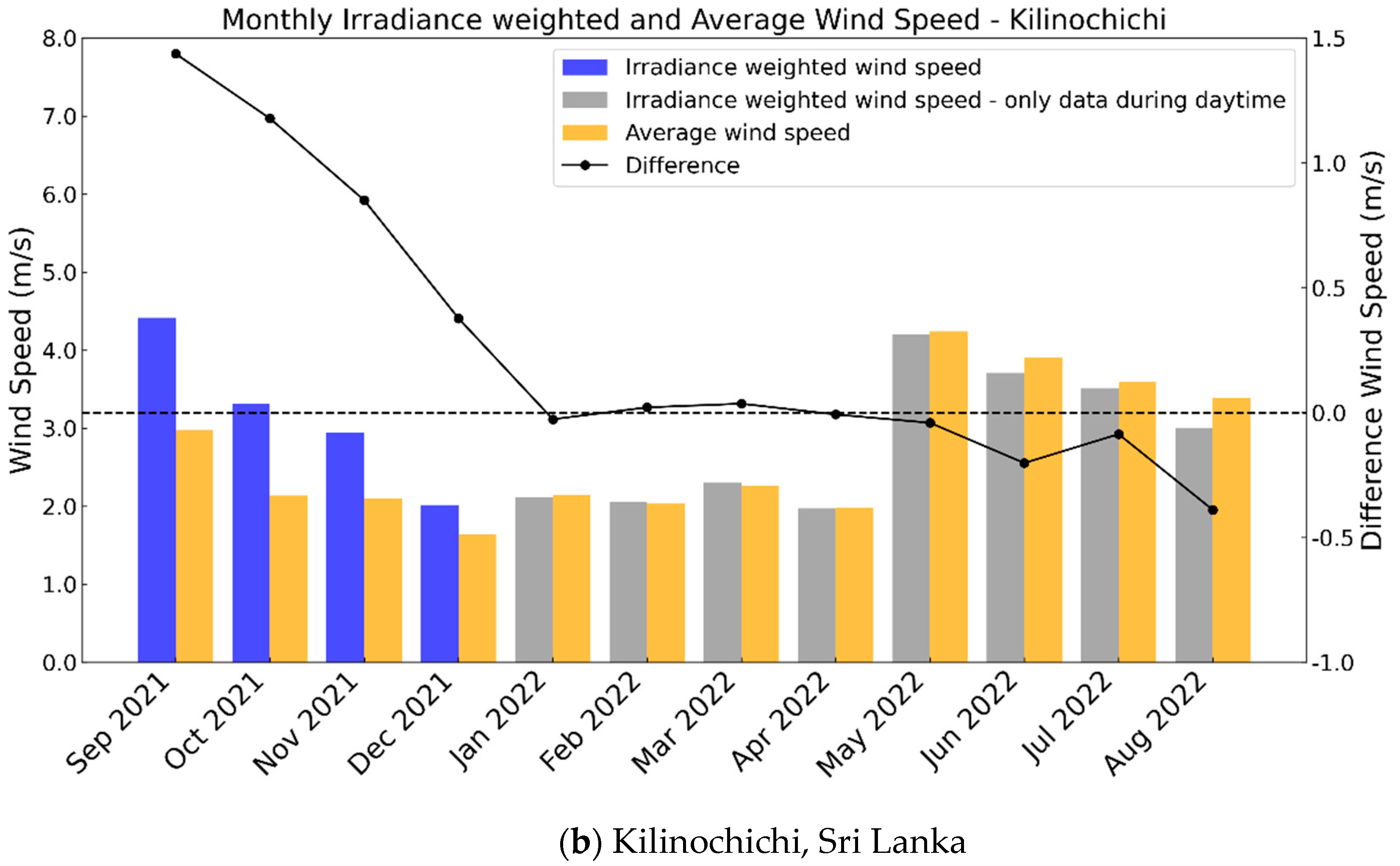
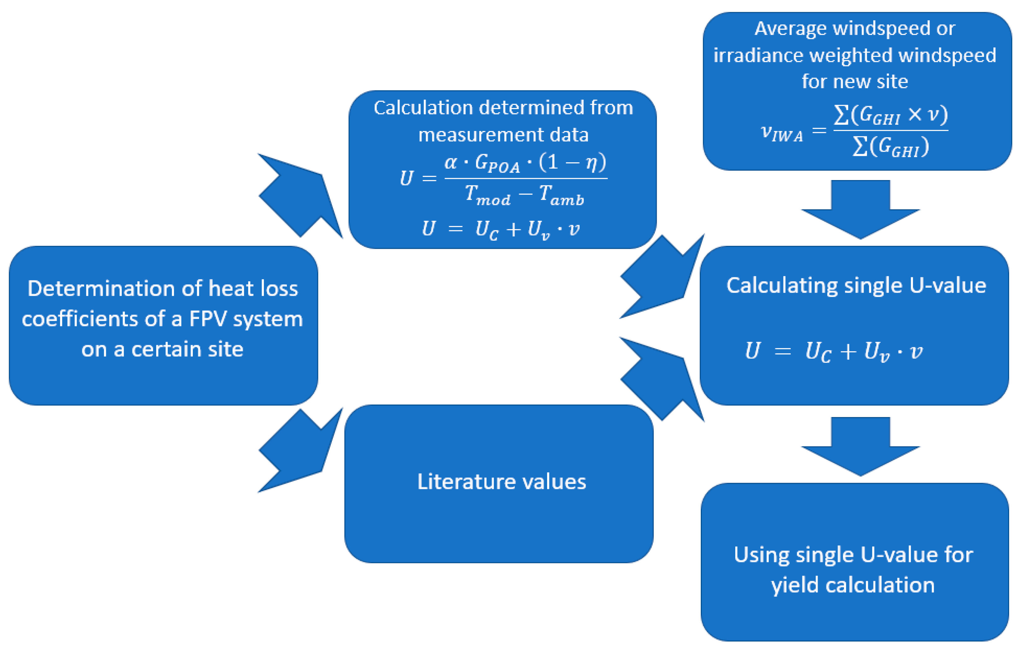
3.2. Irradiance Weighted Wind Speed

As the operating temperature is dependent on wind speed, accounting for the wind speed at site is necessary for an accurate estimation of operating temperature. In many of the EYA tools, this is not possible in the current versions of the software. Note that PVsyst allows for setting a value for the wind-dependent heat loss coefficient, but that this is not recommended unless appropriate wind speed values for the site are used. Currently, the wind speeds provided in the default meteorological datasets are not sufficiently accurate and own values must be uploaded. Here, we introduce a more simplified method to account for the windspeed at site, but allow for the application of only one heat loss coefficient in the EYA calculations. For this, we suggest that the single U-value be computed through:

$$U=U_C+U_v\times v_{IWA}$$

(6)

where v_IWA is the irradiance weighed wind speed given by:

$${\nu }_{IWA}=\frac{{{\displaystyle \sum }}^{ }\left(G_{GHI}\times \nu \right)}{{{\displaystyle \sum }}^{ }\left(G_{GHI}\right)}$$

(7)

where ν is the height adjusted hourly wind speed and G_GHI is the hourly global horizontal irradiance. We suggest using the irradiance weighed average instead of the normal average to only include windspeed during the daytime and account for potential covariance between wind speed and irradiance. In Figure 7a, the monthly average windspeed and the monthly irradiance weighted windspeeds at a height of 10 m for the site of Oostvoorne in the year 2022 are shown. During the summer months, the irradiance weighted windspeed is typically up to 0.5 m/s higher compared to the average windspeed. However, in the winter months, we observe that the average windspeed is much closer to or even larger than the irradiance weighted windspeed. Figure 7b shows the monthly average windspeeds and the monthly irradiance weighted windspeeds at a height of 10 m for the site of Kilinochichi from September 2021 to September 2022. For this site, the difference shows variations between higher irradiance weighted windspeed and the average wind speed, with the largest difference in September 2021 of 1.4 m/s difference. The difference in wind speed is to a large degree due to calm conditions during the night. Note that for the months in 2022, only daytime values are available; therefore, the difference between the irradiance weighed wind speed and the average wind speed no longer reflects the calm conditions during nighttime. As shown in Figure 5 and Figure 6, where the measured temperatures are compared with the modeled temperatures, an offset of 1 m/s wind speed can result in a temperature offset of between 1.8–3%; thus, applying an irradiance weighted wind speed can improve the accuracy of the modeled temperature.

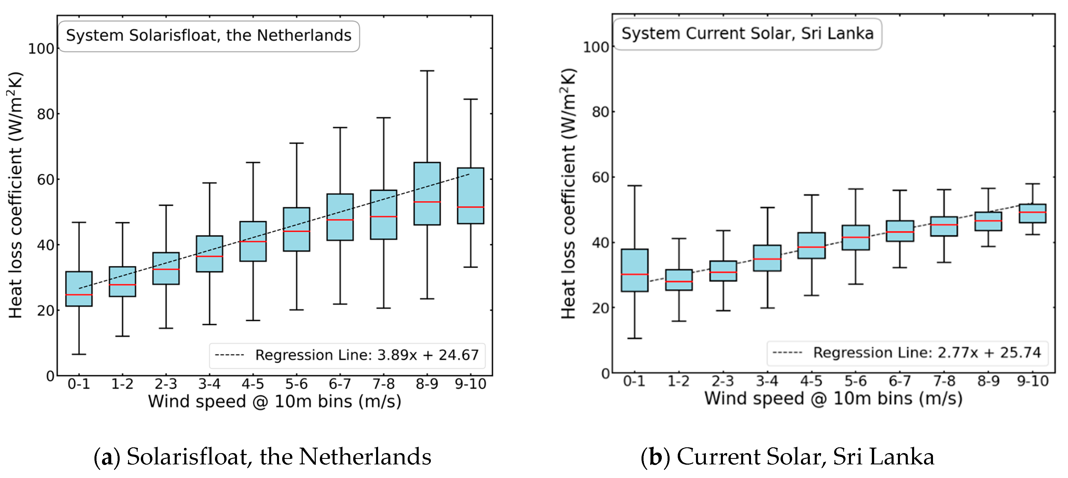
3.3. Heat Loss Coefficients

We conducted calculations to determine the heat loss coefficients, referred to as U-values, for the systems situated in The Netherlands and Sri Lanka. Equation (2) was used for this purpose. The U-values were decomposed into wind-independent U_c and wind-dependent U_v coefficients. The determination of these coefficients was achieved through a linear regression analysis, where the U-value was regressed against the corresponding wind speed. Prior to analysis, the recorded wind speeds were adjusted to a standardized height of 10 m using Equation (5). Figure 8 presents the outcomes of the linear regression analyses, showcasing both the resulting heat loss coefficients and their classification into wind speed bins of 1 m/s. Notably, the U_c values were computed as 24.7 W/m²K and 25.7 W/m²K for The Netherlands and Sri Lanka, respectively. Correspondingly, the U_v values were observed at 3.9 W/m³Ks and 2.8 W/m³Ks for the respective locations. The spread in value for heat loss coefficients per binned wind speed is likely due to the effect from parameters influencing the heat loss of the system that are not accounted for in this simplified thermal model. Remarkably, despite substantial divergences in system design and airflow permeability between the two systems, both exhibited heightened susceptibility to convective cooling induced by wind. This sensitivity exceeded that of the default combination of U_c and U_v values, as identified within the PVsyst context, which are 25 W/m²K and 1.2 W/m³Ks for U_c and U_v, respectively; see Table 1. It should be noted that the U_v value holds greater relevance for systems situated in regions characterized by high wind conditions, such as expansive open water areas for FPV systems.

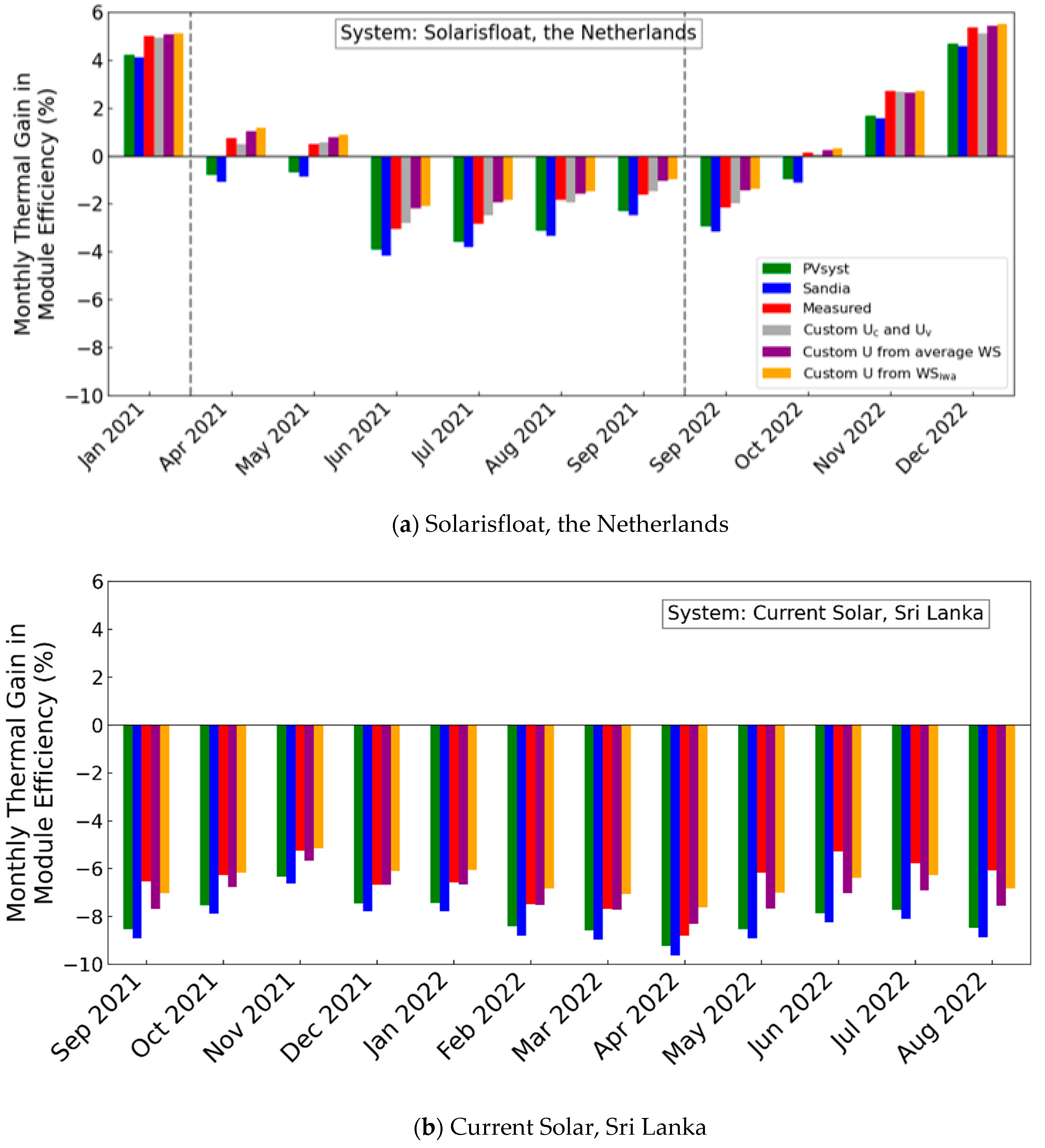
3.4. Thermal Loss Calculation Using Commercial Software

As the module efficiency is directly related to the operating temperature through the module power temperature coefficient, any deviation from the Standard Test Condition (STC) temperature of 25 °C results in a thermal gain for lower temperatures or a thermal loss for higher temperatures. To correctly account for this in the energy yield assessment, the operating temperature must be modeled as correctly as possible for the given system and local conditions. For this modeling, it is most accurate to consider a time series of wind speed values and apply the respective U_c and U_v values found for similar FPV system technologies. However, a reliable time series of wind speed in the available typical meteorological year for a given location is often not available. Therefore, for practical purposes, we compare two approaches in order to consider average wind speed values on site, but where only one single heat loss coefficient is applied in the energy yield assessment, thus eliminating the need for uploading separate wind data to the software. A flowchart that illustrates the methodology can be found in Figure 9. For the first approach, the operating temperature is calculated in, for example, PVsyst, through establishing a single U-value for the given site: U = U_c + U_v × v_AW, where U_c and U_v are found by linear regression of the computed heat loss coefficients, as shown in Figure 8, and the v_AW is yearly average wind speed on site. For the second alternative, the average wind speed is replaced by the irradiance weighted wind speed [Equation (7)]. Both heat loss coefficients are shown in

Table 2. A summary of the determined heat loss coefficients derived from the two respective sites, which form the basis for the thermal loss calculations.

Method	U-Value The Netherlands [W/m2K]	U-Value Sri Lanka [W/m2K]
Custom U (Average WS)	39.5	33.2
Custom U (WSIWA)	40.6	37.9

for both sites.

Figure 10 shows the average monthly thermal gain in module efficiency for the two systems using measured and modeled operating temperatures. This was done by calculating the operating efficiency based on the temperatures and weighing the calculated efficiency with the irradiance. A temperature coefficient of −0.36% per degree Celsius was assumed and a module efficiency of 18.9% at STC. In both locations, employing either the PVsyst or Sandia temperature model without accounting for wind speed results in an overestimation of thermal loss when compared to the utilization of measured temperature values. For the Current Solar system in Sri Lanka, the difference ranges from 0.4% for periods with lower wind speeds to 3% in September and May, when the wind speeds are higher. This difference in thermal gain will directly influence the energy yield assessments in the same order. Applying a heat loss coefficient where the site-dependent wind speed has been taken into account reduces the difference in thermal losses; however, there are still seasonal differences, as the wind speed varies with the seasons. For the system in The Netherlands, the use of a single U-value determined with a yearly averaged windspeed shows the smallest difference in thermal loss compared with the measured temperatures.

To gain insight into the implications of these diverse module efficiencies on yield variations, we calculated the specific yield by multiplying the temperature-corrected module efficiency with the solar irradiance. This computation was carried out over the months, as depicted in Figure 10. The result can be found in

Table 3. Impact on the modeled specific yield by making use of the different temperature models.

Temperature Model	Specific Yield Netherlands [kWh/kWp]	Specific Yield Sri Lanka [kWh/kWp]
Measured Temperatures	1036	1111
PVsyst	1021 (−1.4%)	1095 (−1.4%)
Sandia	1019 (−1.6%)	1090 (−1.9%)
Custom U (Average WS)	1037 (0.1%)	1105 (−0.5%)
Custom U (WSIWA)	1038 (0.1%)	1112 (0.1%)

. It can be observed that both for the system in The Netherlands and the system in Sri Lanka, the yield is most underestimated when the standard Sandia model is applied. The difference in comparison to the yield calculated using measured temperatures amounts to 1.6% and 1.9%, respectively. For temperatures determined using the PVsyst model, the calculated yield is underestimated by 1.4%. Utilizing the method to calculate the U-value, when working with the average monthly wind speed, it is noted that the specific yield for the system in The Netherlands is slightly overestimated, resulting in a difference of 0.1%. This method slightly underestimates temperatures for the Sri Lanka system, with a yield difference of −0.5% compared to the yield calculated using measured temperatures. Lastly, for the U-value determined using the monthly irradiance-weighted U-value, a difference of 0.1% is observed for both The Netherlands and Sri Lanka systems. It is important to highlight that for The Netherlands-based system, the months are not continuous. For the system in Sri Lanka, there are some gaps present in the dataset, preventing us from asserting that this represents the specific yield over an entire year. Therefore, the focus here is on the distinctions between the specific yield of the various models.

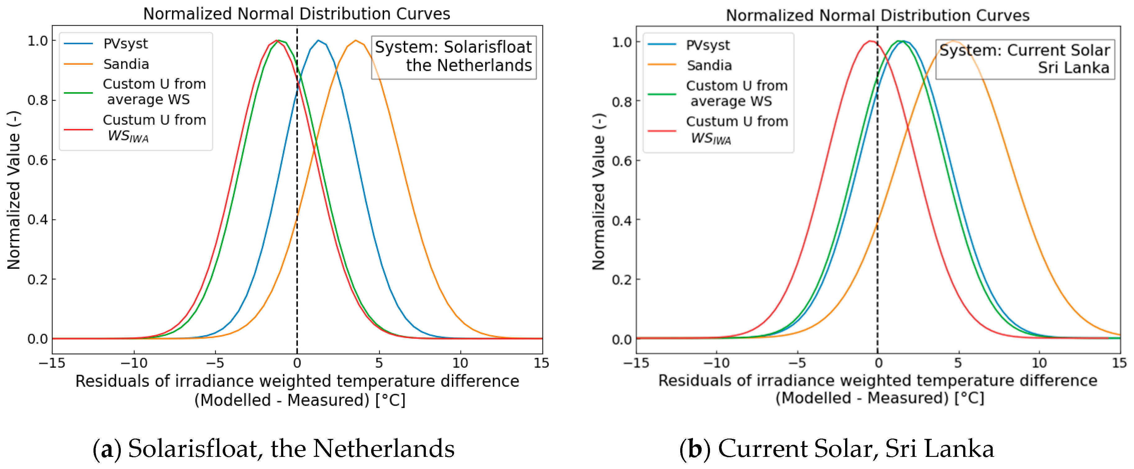
3.5. Comparative Analysis of Models through Residual Examination

An irradiance-weighted residual analysis was performed to examine the disparity between the modeled module temperatures and the measured module temperatures.

Table 4. Residual analysis of the difference in module temperature between the measured temperature values and modeled temperature values. The mean value of the irradiance weighted residual dataset is presented together with the standard deviation of the normal distribution.

Temperature Model	Mean Value Weighted Residual Analysis NL [°C]	SD Normal Distribution NL [°C]	Mean Value Weighted Residual Analysis SL [°C]	SD Normal Distribution SL [°C]
PVsyst	1.00	2.3	1.11	2.78
Sandia	2.15	2.7	2.79	3.44
Custom U (Average WS)	−0.21	2.4	0.95	2.75
Custom U (WSIWA)	−0.36	2.4	−0.03	2.74

presents the weighted average residuals for the various models. For both systems, it is evident that the Sandia model overestimates temperatures by more than 2 degrees Celsius. The PVsyst model, on the other hand, overestimates temperatures by around 1 °C for both systems. In the case of The Netherlands system, both the modeled temperatures using the U-value determined with the average monthly wind speed and the modeled temperatures using the U-value determined with the irradiance-weighted average wind speed U-value exhibit minor deviations of up to approximately 0.4 degrees Celsius. For the Sri Lanka system, the model utilizing irradiance-weighted wind speed for calculating the U-values performs better compared to the temperatures determined using the U-value derived from the average wind speed. This suggests a climate-dependent relationship. Notably, the variations in wind speed during the day and night are more pronounced in Sri Lanka as compared to the Dutch climate, as depicted in Figure 8. Moreover, Table 4 contains the standard deviations of the normal distributions associated with the various models. These standard deviations are also illustrated in Figure 11. It becomes apparent that for both systems, the data dispersion when employing the Sandia model is notably greater in comparison to the other models.

4. Conclusions and Discussion

In this work, measured and modeled module temperatures and computed heat loss coefficients from two different sites with different climate conditions, technologies, and type of water body are presented. Results from both sites show that the wind is an important parameter when estimating the operating temperature for these systems. However, as most energy yield assessment tools do not consider the wind, the operating temperature can be overestimated, thus leading to overestimating the thermal losses. This specifically holds true for FPV systems, where high wind conditions can occur. For both examined systems, using the commonly applied thermal models from PVsyst and Sandia without considering wind speed results in a overestimation in operating temperature of approximately 2−3% for each 1 m/s of increase in wind speed.

To address the impact of the wind speed on site, we suggest a method whereby, instead of needing to upload a full time series of wind measurements into the EYA analysis, the single heat loss coefficient is adjusted to the average windspeed or the irradiance weighted wind speed at 10 m height. Applying the irradiance weighted wind speed has an advantage, as it considers the wind speeds that are dominant when the energy production is at its highest. Our work shows that the wind speed can be higher during daytime, and it can therefore give a more realistic average wind speed during operational hours. The methods presented in this work allow for a more simplified adjustment to local conditions, which for locations with wind speeds higher than 1 m/s will reduce the miscalculation of thermal loss. It should be noted that as this method uses an average yearly value, seasonal differences are not considered. This is shown in Figure 8, where the deviation in thermal loss when compared to measured values ranges from 3% in periods with high winds compared to 0.3% during periods with lower winds. Still, the overall energy yield is more accurately computed when applying a wind speed-adjusted heat loss coefficient compared to the suggested default values. Additional research is needed to enhance the understanding of heat loss coefficients for different system types in various climate conditions and to assess the proposed methodology for alternative systems. This will establish a stronger foundation for selecting appropriate heat loss coefficients in EYA for new sites. It should be mentioned that this is planned to be addressed through the international collaboration within IEA PVPS Task 13, in the subtask addressing energy yield models for FPV.

References

1. Skoplaki, E.; Palyvos, J.A. Operating temperature of photovoltaic modules: A survey of pertinent correlations. Renew. Energy 2009, 34, 23–29. [Google Scholar] [CrossRef]
2. Liu, H.; Krishna, V.; Lun Leung, J.; Reindl, T.; Zhao, L. Field experience and performance analysis of floating PV technologies in the tropics. Prog. Photovoltaics Res. Appl. 2018, 26, 957–967. [Google Scholar] [CrossRef]
3. Kjeldstad, T.; Lindholm, D.; Marstein, E.; Selj, J. Cooling of floating photovoltaics and the importance of water temperature. Solar Energy 2021, 218, 544–551. [Google Scholar] [CrossRef]
4. Lindholm, D.; Kjeldstad, T.; Selj, J.; Marstein, E.S.; Fjær, H.G. Heat loss coefficients computed for floating PV modules. Prog. Photovoltaics Res. Appl. 2021, 29, 1262–1273. [Google Scholar] [CrossRef]
5. Kamuyu, W.C.L.; Lim, J.R.; Won, C.S.; Ahn, H.K. Prediction model of photovoltaic module temperature for power performance of floating PVs. Energies 2018, 11, 447. [Google Scholar] [CrossRef]
6. Hayibo, K.S.; Mayville, P.; Kailey, R.K.; Pearce, J.M. Water Conservation Potential of Self-Funded Foam-Based Flexible Surface-Mounted Floatovoltaics. Energies 2020, 13, 6285. [Google Scholar] [CrossRef]
7. Kaplanis, S.; Kaplani, E.; Kaldellis, J.K. PV Temperature Prediction Incorporating the Effect of Humidity and Cooling Due to Seawater Flow and Evaporation on Modules Simulating Floating PV Conditions. Energies 2023, 16, 4756. [Google Scholar] [CrossRef]
8. IEC 61853-2; Photovoltaic (PV) Module Performance Testing and Energy Rating—Part 2: Spectral Responsivity, Incidence Angle and Module Operating Temperature Measurements. IEC: Geneva, Switzerland, 2018.
9. Faiman, D. Assessing the outdoor operating temperature of photovoltaic modules. Prog. Photovoltaics Res. Appl. 2008, 16, 307–315. [Google Scholar] [CrossRef]
10. Barykina, E.; Hammer, A. Modeling of photovoltaic module temperature using Faiman model: Sensitivity analysis for different climates. Sol. Energy 2017, 146, 401–416. [Google Scholar] [CrossRef]
11. Ghabuzyan, L.; Pan, K.; Fatahi, A.; Kuo, J.; Baldus-Jeursen, C. Thermal effects on photovoltaic array performance: Experimentation, modeling, and simulation. Appl. Sci. 2021, 11, 1460. [Google Scholar] [CrossRef]
12. Koehl, M.; Heck, M.; Wiesmeier, S.; Wirth, J. Modeling of the nominal operating cell temperature based on outdoor weathering. Sol. Energy Mater. Sol. Cells 2011, 95, 1638–1646. [Google Scholar] [CrossRef]
13. King, D.L.; Boyson, W.E.; Kratochvill, J.A. Photovoltaic Array Performance Model; Sandia National Laboratories: Albuquerque, NM, USA, 2004. [Google Scholar] [CrossRef]
14. Dörenkämper, M.; Wahed, A.; Kumar, A.; De Jong, M.M.; Kroon, J.; Reindl, T. The cooling effect of floating PV in two different climate zones: A comparison of field test data from The Netherlands and Singapore. Sol. Energy 2021, 214, 229–247. [Google Scholar] [CrossRef]
15. PVsyst: Array Thermal Losses. Available online: https://www.pvsyst.com/help/thermal_loss.htm (accessed on 14 August 2023).
16. Holmgren, W.F.; Hansen, C.W.; and Mikofski, M.A. pvlib python: A python package for modeling solar energy systems. J. Open Source Softw. 2018, 3, 884. [Google Scholar] [CrossRef]
17. Holton, J.R.; Hakim, G.J. Wind and Wind Systems. In Introduction to Dynamic Meteorology; Elsevier Academic Press: Amsterdam, The Netherlands, 2013; ISBN 9780123848666. [Google Scholar]
Figure 1. Contour plots showcasing the modeled module temperature variations with adjusted constants in the PVsyst (a) and Sandia (b) temperature models. Ambient temperature set at 20 °C, and the plane of array irradiance of 800 W/m2.
Energies 16 07153 g001
Figure 2. The Solarisfloat system located in lake Oostvoorne, The Netherlands. (a) Satellite image of Lake Oostvoorne and (b) aerial view of the Solarisfloat system.
Energies 16 07153 g002
Figure 3. The Current Solar system in the small pond located outside Jaffna University, Kilinochchi, Sri Lanka. (a) Satellite image of pond with FPV system in Kilinochchi, Sri Lanka and (b) picture of the Current Solar system. Position of system denoted by a star.
Energies 16 07153 g003
Figure 4. Direct side-by-side comparison of modeled and measured module temperatures across a few representative days, encompassing systems in The Netherlands (a) and Sri Lanka (b).
Energies 16 07153 g004
Figure 5. Scatterplots with the modeled temperature data of PVsyst and Sandia versus the measured temperature data of the Solarisfloat system in The Netherlands. The colors represent the wind speed at a height of 10 m (a,c). Boxplots with the temperature difference (modeled temperature—measured temperature) as a function of wind speed bins. Furthermore, the result of a linear regression on these full datasets can be observed (b,d).
Energies 16 07153 g005
Figure 6. Scatterplots with the modeled temperature data of PVsyst and Sandia versus the measured temperature data of the Current Solar system in Sri Lanka. The colors represent the measured wind speed (a,c). Boxplots with the temperature difference (modeled temperature—measured temperature) as a function of wind speed bins. Furthermore, the result of a linear regression on these full datasets can be observed (b,d).
Energies 16 07153 g006
Figure 7. Average monthly wind speed in orange and the irradiance weighted wind speed in blue for the Oostvoorne site in The Netherlands (a) and the Sri Lanka site (b).
Energies 16 07153 g007aEnergies 16 07153 g007b
Figure 8. Heat loss coefficients plotted as a function of wind speed bins at 10 m height for Solarisfloat system in The Netherlands (a) and the Current Solar system in Sri Lanka (b). Furthermore, the result of a linear regression on these full datasets can be observed. The box plot represents the interquartile range of the binned datapoints, the line is the median, and the whiskers show the range of the data.
Energies 16 07153 g008
Figure 9. Flowchart diagram illustrating the methodology for the calculation of a singular U-value for site assessment while considering local wind parameters.
Energies 16 07153 g009
Figure 10. Monthly average enhancement in module efficiency for the systems located in The Netherlands (a) and Sri Lanka (b), employing both measured and modeled operational temperatures. The dotted lines in the top figure indicate two cuts in the dataset.
Energies 16 07153 g010
Figure 11. The normalized normal distribution curves showcase irradiance-weighted residuals between modeled and observed temperatures for various models at both The Netherlands (b) and Sri Lanka (a) locations. A positive temperature differential indicates an elevation in temperature relative to the measured value.
Energies 16 07153 g011