Article

The Development of a Transient Analysis Platform of Near-Critical CO2 Thermodynamic Systems via an Enthalpy-Based Implicit Continuous Eulerian Approach

1
Department of Convergence and Fusion System Engineering, Kyungpook National University, Sangju 37224, Republic of Korea
2
Korea Atomic Energy Research Institute, Daejeon 34057, Republic of Korea
*
Author to whom correspondence should be addressed.
Energies 2024, 17(5), 1126; https://doi.org/10.3390/en17051126
Submission received: 30 January 2024 / Revised: 20 February 2024 / Accepted: 25 February 2024 / Published: 27 February 2024
(This article belongs to the Special Issue Advances in Supercritical CO2 Power Cycle Applications)

Abstract

:
This work presents the development and validation of an enthalpy-based implicit continuous Eulerian (ICE) solver, termed the near-critical ICE solver (NICES), for the analysis of near-critical CO2 thermodynamic systems. Traditional approaches relying on pressure and temperature as main inputs for the analysis have limitations in handling CO2 near the critical point, which exhibits unique characteristics and frequent phase changes. To overcome these limitations, this study proposes using enthalpy as a more suitable mathematical modeling approach. The NICES methodology employs the homogeneous equilibrium model and the Span and Wagner equations of state for CO2. This solver demonstrates improved numerical stability and computational speed compared to explicit calculation methods, as validated by frictionless heated pipe scenarios involving phase transitions near the critical point. The enthalpy-based NICES platform can predict thermohydraulics, including multiphase flows, without requiring specialized two-phase flow models.

1. Introduction

The term “supercritical” describes a special type of material phase. Above critical conditions (temperature and pressure), the meniscus between liquid and gas phases disappears, and the material behaves with unique characteristics that are neither similar to liquid nor gas phases [1]. This supercritical phenomenon is a secondary phase change, not an additional primary phase change phenomenon such as boiling or condensing. At the critical point, a physical singularity, the material’s second-order derivative of free energy, such as specific heat capacity, is discontinuous. Figure 1 illustrates that the fluid undergoes drastic property changes near the critical point. These unique characteristics have valuable engineering applications. For example, near the critical point, the compressibility factor is low, similar to that of a liquid, making it easy to compress as a pump. Additionally, heat exchangers for waste heat recovery can be designed across the critical point without considering internal boiling or condensing. Carbon dioxide (CO2) is one of the most promising supercritical fluids for engineering applications, as its critical conditions (approximately 31.4 °C and 7.4 MPa) are easily accessible. Due to the useful characteristics of near-critical CO2, numerous attempts using it have been made to improve thermodynamic systems such as improving power conversion systems (called S-CO2 systems) [2,3,4], thermal energy storage [5,6,7,8] and compressed CO2 energy storage [9,10,11].
In common with other thermodynamic energy systems, systems utilizing the thermodynamic properties of near-critical CO2 are subject to various issues that require transient analysis, including start-up and shutdown procedures, output alterations, accidents in power generation systems, and charging and discharging situations in energy storage systems. However, rapid property changes lead to poor convergence and reduce the numerical stability of fluid transient analysis methodologies. In addition, due to the unique properties of CO2 near the critical point, the numerical analysis of systems employing it presents several challenges for engineers.
To date, some work has been carried out to develop platforms to analyze transients in supercritical CO2 power systems. However, only some platforms have been developed specifically for the analysis of supercritical CO2 transients, and most have been modified and adapted from platforms developed for the analysis of other systems. One example of a program developed solely for analyzing S-CO2 systems is the Argonne National Laboratory’s PDC (Plant Dynamics Code) [12]. This program uses temperature, pressure and mass flow rate as the base variables, and the Taylor series method as the numerical scheme [13]. However, the system is intended to analyze supercritical single phases and was developed without the goal of two-phase flows. Therefore, it is not directly applicable to the analysis of transcritical systems, where two-phase flows near the critical point are more likely to be considered, or compressed CO2 energy storage systems, where liquid carbon dioxide is considered rather than a supercritical CO2 power cycle.
For instance, in the context of an advanced system leveraging the near-critical thermodynamic behavior of CO2, such as an oxy-combustion cycle integrated with an air separation unit (ASU)—it may be feasible to utilize a low-temperature heat sink, i.e., a compressed CO2 energy storage system that charges energy in the liquid state of CO2. Such a system could enhance overall efficiency by exploiting lower temperatures or harnessing the latent heat of liquid CO2 near the critical point. In this scenario, it may be possible to compress the low-temperature component from the liquid state to the supercritical phase, resulting in a phase transition of liquid CO2 to the supercritical phase as it is heated within the compressor or a recuperator. There is significant potential for engineering applications involving two-phase CO2 near the critical point. Although research efforts are currently underway to develop condensation models from the phenomenological perspective of individual components [14,15], a notable gap remains in the development of specialized analysis platforms to address such systems from a holistic standpoint.
In cases where multiphase flows need to be considered or PDC codes are unavailable, most of the transient analysis was performed by borrowing safety analysis codes from nuclear systems. Techniques to simulate the entire plant in 1D have been well studied for nuclear systems, which are often deeply analyzed for two-phase flows, including boiling, and the need to analyze and predict sudden transient states such as accidents. As part of these studies, S-CO2 physical properties were inserted into MARS-KS [16,17], a code for analyzing light water reactors, to perform a transition analysis and GAMMA+ [18,19,20], and a code for analyzing high-temperature gas reactors, to perform a transient analysis. Both nuclear codes analyze numerically, based on temperature, pressure and velocity, and use the implicit continuous Eulerian methodology (ICE) [21]. The ICE methodology is a semi-implicit method that allows some explicit terms in the governing equations, which speeds up the computation by enclosing all variables in the next timestep as a function of pressure and solving the matrix for pressure. This method is often used to solve fluid equations that would require excessive computation time if solved explicitly [22,23,24,25,26].
Previous studies on CO2 near the critical point have primarily relied on pressure and temperature as the basis for analysis. When two-phase flows were considered, researchers divided gas–liquid mixtures into liquid and gas phases, using models such as the two-fluid two-phase model [27] or the drift flux model [28]. However, there may be better approaches for dealing with CO2 near the critical point. Some properties reduced drastically near the critical point and eventually became zero above the critical point (Figure 2). Latent heat is one of these properties. Due to the latent heat being very low near the critical point, frequent phase changes occur near the critical point. Not only gases and liquids, but also supercritical phases can be mixed and utilized due to the near-critical condition. Thus, using temperature as a nondifferentiable variable in the phase transition process may be unsuitable because the temperature during the phase transition stays constant, so it is on a nondifferentiable basis. Therefore, we propose using enthalpy as a more appropriate mathematical modeling approach, despite the increased computational requirements. First, enthalpy is always differentiable for energy flows in and out. Second, near the critical point, the surface tension and density difference between the liquid and gas phases are very low, resulting in distinct behavior from typical two-phase flows. Therefore, it is a useful assumption that every velocity, temperature and pressure of the gas and liquid phase are equal for near-critical CO2 flows. Sung Jun Bae et al. [29] showed that multiphase flows near the critical point could be approximated as a single phase without significant errors. Thus, the homogeneous equilibrium model (HEM) is suitable for analyzing such flows. HEM assumes that both phases have the same velocity, temperature and pressure using average physical properties between the two phases determined by considering the vapor fraction. For the same reason, this model is the easiest to embed when building a coding platform based on enthalpy. This is because as the phase transition occurs, the temperature stays the same, but the enthalpy keeps changing, so using enthalpy instead of temperature eliminates the need to track the vapor fraction separately.
This study presents an enthalpy-based methodology for analyzing the near-critical CO2 transient, named near-critical implicit continuous Eulerian solver (NICES) that considers this. The numerical solution uses the ICE method with pressure, mass flow rate and enthalpy as the basis of governing equations. Specific differentiation methods and implementations utilizing these foundations and methodologies are described in detail. Equations of state (EOS) of the CO2, especially near the critical point, utilize the Span and Wagner EOS model [30] from the CoolProp database [31]. The Span and Wagner EOSs internally perform iterative computation for convergence, which consumes a lot of computational resources, but in this study, the EOSs are adopted as they are, and approximations related to physical properties are not considered.
The method applied in this study, which utilizes an enthalpy-based governing equation to achieve numerical stability using an intrinsic HEM model in the transition analysis of near-critical fluids, has not yet been applied in the field of supercritical CO2 transition analysis. There are still very few transient analysis platforms that include CO2 properties near the critical point in the form of property modules rather than property tables or constants, and they either do not address the multiphase flow regime or do so at the expense of a lot of numerical instability. The attached paper is an example of CFD analysis, which is difficult to apply to 1D analysis of the entire plant system, especially when analyzing accidents or transients. From a technical point of view, this problem is a bottle neck in the field of supercritical CO2 power generation systems and must be solved for future trans-critical system applications.

2. Governing Equation of a Near-Critical CO2 System

2.1. Partial Differential Equation Form

It is crucial to consider equations with compressible fluids to analyze thermodynamic systems on the development platform. Therefore, the primary governing equation used in this study is adopted from previous research conducted by PDC [12]. In Figure 3, a heated pipe is used to model the pipe flow of the compressible fluid. The dynamic behavior of the flow in the pipe can be described by three conservative equations: continuity, momentum and energy. Furthermore, according to the previous research by Hewitt et al. [32] and Yan et al. [33], conservation equations can be written in simplified partial differential equation form, as shown in Equations (1)–(3).
Continuity,
ρ t + z ρ V = 0
Momentum,
( ρ V ) t + z ρ V V = P z ρ g ρ f V 2
Energy,
( ρ H ) t + z ρ H V = q z q w
It should be noted that the equations utilized in this study are derivatives of previous research by Moisseytsev et al. [12], with some modifications made to ensure platform expandability.
-
Gravitational effects are ignored.
-
Stress is represented by the friction at the wall only.
-
Acceleration pressure drop is ignored.
-
Energy loss via friction and form loss are ignored.
-
The kinetic energy of the fluid is neglected; this means that the total energy of the compressible fluid is represented via enthalpy. As a result, all pressures are considered total pressure.
-
Upwind scheme is applied: Major transport properties (density and enthalpy) are transferred along the flow direction. Note: “NOT” transport properties (such as area and discretized length) are used as the mean values.

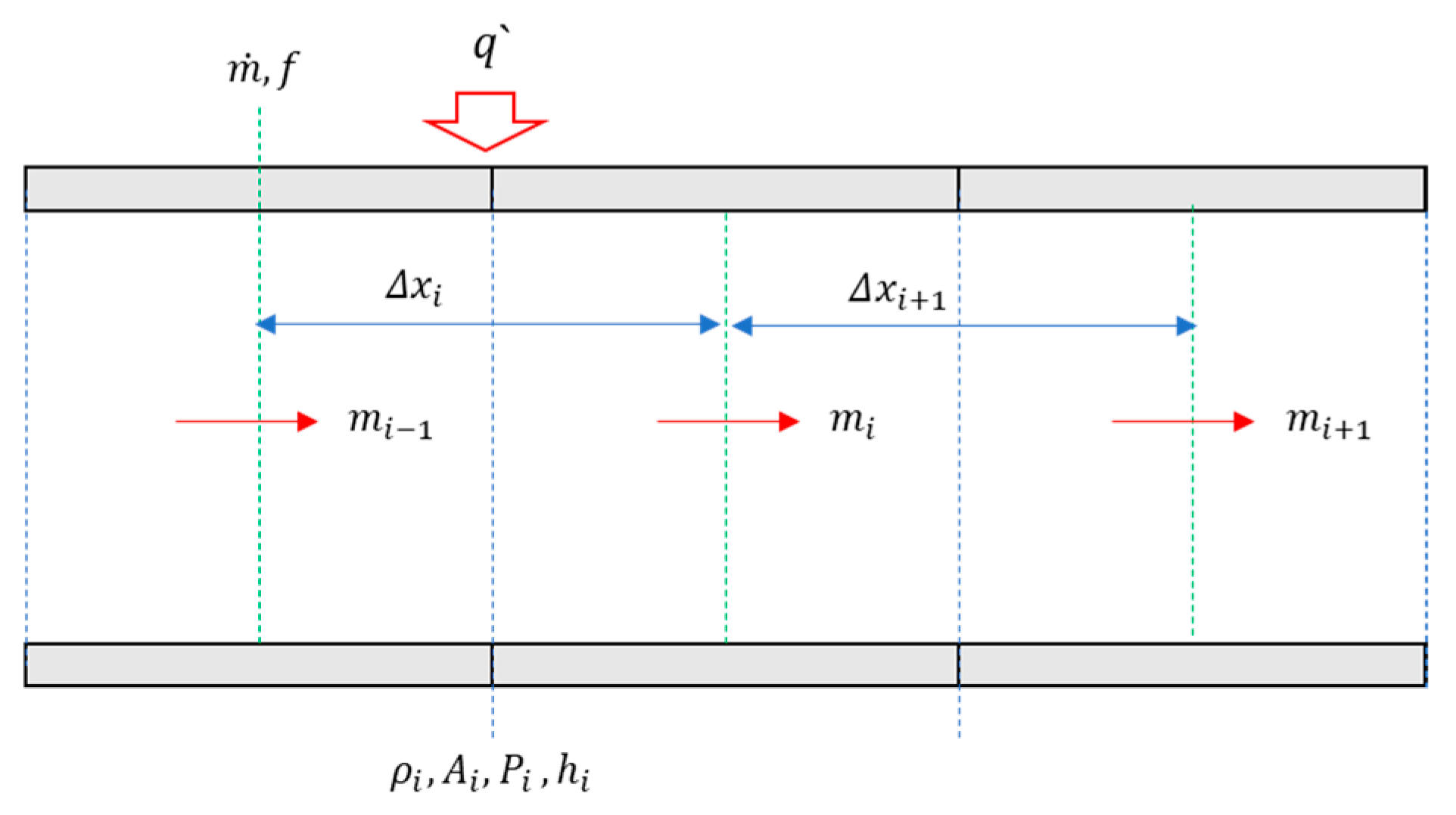
2.2. Spatial Discretization

To numerically solve a system of conservation Equations (1)–(3), the given partial differential equations must be discretized. Discretization is a crucial step, and one of the most important issues to consider is the handling of momentum conservation in Equation (2). The pressure difference between the inlet and outlet induces the flow rate. Therefore, defining the mass flow rate at the same position as the other parameters, such as density, pressure and enthalpy, can increase numerical instability. In this case, the “staggered mesh” approach is applied to handle it. This method reduces numerical instability by intersecting vector and scalar properties. In this case, the transport properties are assumed to borrow the values from the donor channel.
Figure 4 illustrates the staggered mesh batch for the given situation. Under these staggered mesh conditions, Equations (1)–(3) are again discretized as Equations (4)–(6).
ρ i t = m ˙ i 1 m ˙ i A i Δ x i
m i ˙ t = P i P i + 1 2 A i Δ x i + Δ x i + 1 2 f i A i ρ i m ˙ i 2
h i t = m ˙ i 1 + m ˙ i 2 M i h i 1 h i + q M i Δ x i M i = A i ρ i Δ x i
Numerical integration can discretize Equations (4)–(6) and solve them explicitly. However, when solving thermo-fluid systems, the required time intervals for numerical stability must be longer. As a result, excessive computation is necessary, making it impossible to analyze complex plant systems in a physically feasible time frame.
We propose a method that reduces the computation required to address this issue. Specifically, we apply the implicit continuous Eulerian (ICE) semi-implicit method. By doing so, we can overcome the excessive computation required for explicit methods and effectively analyze the transitions of complex plant systems in a reasonable computational time.

3. Numerical Method

3.1. Implicit Continuous Eulerian Method

The ICE method is a numerical approach that can be used to analyze transient thermohydraulic systems. This method is a semi-implicit method, which combines the advantages of both implicit and explicit methods [21,22,23,24,25,26].
The ICE method discretizes the system using a continuous Eulerian framework. This means the system is divided into small control volumes that are connected to each other by mass energy and momentum flows. Then, the governing equations for the system are discretized using finite-volume methods, and the resulting algebraic equations are solved iteratively.
In general, the calculation steps for ICE methods are as follows:
(1)
Represent the momentum equation with pressure differences.
(2)
Represent the energy equation with momentum information of the next timestep and existing energy information. In this process, explicit terms were adopted. When put up with this numerical instability, it is possible to represent the energy equation via the pressure of the next timestep.
(3)
Solve the pressure matrix, and iteratively calculate it before convergence.
For the iterative calculation, this study applies the newton method [34] for timestep control. For the calculation, the base properties of a given system ( m ˙ ,   P ,   h ) are linearized as Equation (7).
m i ˙ n + 1 = m i ˙ k + δ m ˙ i     p i n + 1 = p i k + δ p i     h i n + 1 = h i k + δ h i

3.2. General Node

For a typical node that is not an inlet or outlet of a pipe, the momentum equation can be discretized as Equation (8) for solving with the ICE method.
m i ˙ n + 1 m ˙ i n Δ t = P i P i + 1 n + 1 2 A i Δ x i + Δ x i + 1 2 f i n A i ρ i k D h | m ˙ i n | m ˙ i n + 1
In Equation (7), the term  m ˙ i 2  in Equation (5) makes the given equation nonlinear. To achieve fast computational speed at the cost of some numerical instability by linearization, we modified the term to be a combination of explicit and implicit terms as  | m ˙ i n | m ˙ i n + 1 .
Substituting Equation (7) into Equation (8), Equation (9) is obtained.
m i ˙ n + 1 = m i ˙ k + δ m i ˙ = m i ˙ n + 2 A i Δ t Δ x i + Δ x i + 1 P i k + δ P i P i + 1 k δ P i + 1 2 f i n Δ t A i ρ i n D h | m ˙ i n | m i ˙ k + | m ˙ i n | δ m 1 + 2 f i n Δ t A i ρ i n D h | m ˙ i n | δ m i ˙ = m i ˙ n 1 + 2 f i n Δ t A i ρ i n D h m ˙ i n m i ˙ k + 2 A i Δ t Δ x i + Δ x i + 1 P i k P i + 1 k + δ P i δ P i + 1
Equation (9) can be rewritten as Equation (10) to reduce the complexity of the expression.
δ m ˙ i = B i k ~ + C i k ~ δ P i δ P i + 1
where
A i k ~ = 1 + 2 f i n Δ t A i ρ i n D h | m ˙ i n | B i k ~ = m i ˙ n 1 + 2 f i n Δ t A i ρ i n D h m ˙ i n m i ˙ k + 2 A i Δ t Δ x i + Δ x i + 1 P i k P i + 1 k A i k ~     C i k ~ = 2 A i Δ t A i k ~ Δ x i + Δ x i + 1
As shown in Equation (10), treating the discretized equation makes it possible to express mass flow rate changes in the next timestep with the terms of pressure changes.
To utilize Equation (10), the energy equation of Equation (6) can be time-discretized as Equation (11).
h i n + 1 h i n Δ t = h i k h i n + δ h i Δ t = m ˙ i 1 n + 1 + m ˙ i n + 1 2 M i n h i 1 n h i n + q n M i n Δ x i
It should be noted that the term  h i 1 n h i n  is an explicit term for the ICE method, which is described in Section 3.1. Equation (11) can be updated with Equation (7) as Equation (12).
δ h i = h i n h i k + Δ t 2 M i n m ˙ i 1 k + m ˙ i k h i 1 n h i n + q n Δ t Δ x i M i n + Δ t 2 M i n h i 1 n h i n B i 1 k ~ + B i k ~ + C i 1 k ~ δ P i 1 δ P i + C i k ~ δ P i δ P i + 1
Since the continuity equation is about density, it needs further development to represent temperature and enthalpy, which is the basis of this study, as Equation (13).
ρ i n + 1 = ρ i k + ρ P i k δ P i + ρ h i k δ h i
In Equation (13), the terms  ρ i k ρ P i k  and  ρ h i k  can be obtained from the EOS at the given enthalpy and pressure. By applying Equations (7) and (13) to Equation (4), the time–discretized continuity equation can be written as Equation (14).
ρ i k + ρ P i k δ P i + ρ h i k δ h i ρ i n = Δ t A i Δ x i m ˙ i 1 k m ˙ i k + δ m i 1 δ m i
Also, applying Equation (10) to Equation (14) and Equation (15) is induced.
ρ P i k + Δ t A i Δ x i C i 1 k ~ + C i k ~ δ P + ρ h i k δ h = ρ i n ρ i k + Δ t A i Δ x i m ˙ i 1 k m ˙ i k + Δ t A i Δ x i B i 1 k ~ + C i 1 k ~ δ P i 1 Δ t A i Δ x i B i k ~ C i k ~ δ P i + 1
Combining the energy conservation equation of Equation (12) and the continuity equation of Equation (15) yields a matrix equation as Equation (16).
B 11 B 12 B 21 B 22 δ P i δ h i = b 1 b 2 + c 1 c 2 δ P i 1 + d 1 d 2 δ P i + 1
where
B 11 = Δ t 2 M i n h i 1 n h i n C i 1 k ~ C i k ~     B 12 = 1   B 21 = ρ P i k + Δ t A i Δ x i C i 1 k ~ + C i k ~     B 22 = ρ h i k b 1 = h i n h i k + Δ t 2 M i n m ˙ i 1 k + m ˙ i k h i 1 n h i n + q n Δ t Δ x i M i n + Δ t 2 M i n h i 1 n h i n B i 1 k ~ + B i k ~ b 2 = ρ i n ρ i k + Δ t A i Δ x i m ˙ i 1 k m ˙ i k + B i 1 k ~ Δ t A i Δ x i + B i k ~ Δ t A i Δ x i c 1 = C i 1 k ~ Δ t 2 M i n h i 1 n h i n     c 2 = Δ t A i Δ x i C i 1 k ~ δ P i 1     d 1 = C i k ~ Δ t 2 M i n h i 1 n h i n     d 2 = Δ t A i Δ x i C i k ~ δ P i + 1
Multiplying Equation (16) by the inverse of matrix B, a square matrix with a size equal to the number of nodes at about P can be obtained. In solving this “pressure matrix”, every unknown parameter of the system, such as pressures, enthalpies, and mass flow rates, can be updated by Equations (10) and (16). This update is continued before the value  max ( δ P i / P i )  achieves a convergence criterion, which is generally selected as 10−6. If this criterion is achieved, updating  ρ i k ,   P i k ,   h i k  is stopped, and these values are passed to the next timestep.

3.3. Boundary Node

At the inlet (left) boundary condition,  m ˙ i 1  in Equations (4) and (6) should be handled with suitable boundary conditions. Also, in Equation (5), the term  P i + 1  is impossible to calculate without outlet (right) boundary conditions. Therefore, special treatment for the boundary nodes is necessary.
Two kinds of boundary conditions are possible for the inlet boundary condition: the mass flow rate boundary and fluid boundary. Figure 5 shows the inlet boundary node of the given compressible flow in the heated pipe situation.
If the forced mass flow rate of the inlet boundary is given as  m ˙ b , it can be handled simply by alternating  m ˙ i 1 k  in Equation (16) as  m ˙ b . However, if the inlet boundary condition is given as fluid properties such as pressure and enthalpy, the mass flow rate of the inlet boundary  m ˙ b  should be calculated through the momentum equation. For this, momentum equations for the inlet boundary node are expressed in Equation (17).
δ m ˙ b = B b k ~ + C b k ~ δ P 0
where
A b k ~ = 1 + 2 f 0 n Δ t A 0 ρ 0 n D h | m ˙ b n |   B i k ~ = m b ˙ n 1 + 2 f 0 n Δ t A 0 ρ 0 n D h | m ˙ b n | m b ˙ k + A 0 Δ t Δ x 0 P b P 0 k A b k ~       C i k ~ = A 0 Δ t A b k ~ Δ x 0
By applying Equation (17), the time discretized form of continuity and energy equation can be obtained as Equations (18) and (19), via the same method described in Section 3.2.
ρ P 0 k Δ t A i Δ x i C b k ~ C 0 k ~ δ P 0 + ρ h i k δ h = ρ i n ρ i k + Δ t A i Δ x i m ˙ b k m ˙ i k + B b k ~ Δ t A 0 Δ x 0 B 0 k ~ Δ t A 0 Δ x 0 + C 0 k ~ Δ t A 0 Δ x 0 δ P 1
Δ t 2 M 0 n h b h 0 n C b k ~ + C 0 k ~ δ P 0 + δ h 0 = h 0 n h 0 k + Δ t 2 M i n m ˙ b k + m ˙ 0 k h b h 0 n + q n Δ t Δ x 0 M 0 n + Δ t 2 M i n B b k ~ + B 0 k ~ h b h 0 n C 0 k ~ Δ t 2 M i n h b h 0 n δ P 1
Figure 6 shows the outlet boundary nodes. In the case of the outlet boundary, two options of boundary conditions are possible: the mass flow rate boundary and pressure boundary. If the mass flow rate is given as a boundary condition, it can easily handle the boundary conditions with a forced outlet mass flow rate in  m ˙ i  Equation (16). In the case of the pressure boundary, similar to Equations (17)–(19), Equations (20)–(22) should be applied for the outlet pressure boundary condition for momentum, continuity and energy conservation equations, respectively. In Equations (20)–(22), i represents the outlet node.
δ m ˙ i = B i k ~ + C i k ~ δ P i
where
A i k ~ = 1 + 2 f i n Δ t A i ρ i n D h | m ˙ i n | B i k ~ = m i ˙ n 1 + 2 f i n Δ t A i ρ i n D h m ˙ i n m i ˙ k + A i Δ t Δ x i P i k P b A i k ~     C i k ~ = A i Δ t A i k ~ Δ x i
ρ P i k + Δ t A i Δ x i C i 1 k ~ + C i k ~ δ P + ρ h i k δ h = ρ i n ρ i k + Δ t A i Δ x i m ˙ i 1 k m ˙ i k + Δ t A i Δ x i B i 1 k ~ + C i 1 k ~ δ P i 1 Δ t A i Δ x i B i k ~
Δ t 2 M i n h i 1 n h i n C i 1 k ~ C i k ~ δ P i + δ h i = h i n h i k + Δ t 2 M i n m ˙ i 1 k + m ˙ i k h i 1 n h i n + q n Δ t Δ x i M i n + Δ t 2 M i n h i 1 n h i n B i 1 k ~ + B i k ~ + C i 1 k ~ Δ t 2 M i n h i 1 n h i n δ P i 1

3.4. Timestep Control and Algorithm Flowchart

Since the numerical method employed in Section 3.1, Section 3.2 and Section 3.3 involves a semi-implicit approach, it is necessary to exercise caution when selecting the timestep size. Specifically, considering the explicit terms, the timestep is constrained by the following Equation (23), commonly referred to as the “flow limit” [35]. The suitability of these figures is further analyzed in Section 5.
Δ t l i m i t = min Δ x m ˙
The parameter δP determines the convergence of the timestep. If δP is sufficiently small compared to the pressure values, the timestep is deemed to have converged successfully. Conversely, if the iterative calculation for updating δP becomes excessively iterative or if the computation reports convergence failure due to the EOS, the timestep is halved, and the iteration is repeated. The full algorithm flowchart, including these timestep controls, is shown in Figure 7. The proposed algorithm has been implemented using a Python 3.9 [36] environment.

4. Validation with Explicit Calculation

To evaluate the performance of the proposed methodology, we conducted validation with an explicit calculation by comparing its predictions to data generated by a benchmark result with the explicitly calculated result. The example problem is shown in Figure 8. The problem is about flow in a frictionless, heated pipe, and it is assumed that until t = 0, the system has reached a steady state with no heating and an inlet flow rate of 1 kg/s. At t = 0, the inlet flow rate suddenly increased to 1.1 kg/s, and heating of 165 kW/m along the wall began. Under the given condition, for fluid states near the critical point and during a transient situation, a phase transition occurs in the heated pipe, and it becomes a supercritical state.
The explicit calculation was solved by the 2(3) order Runge–Kutta method using the SciPy internal function solve_ivp [37]. In this case, Timestep utilized the value determined inside the function. The results calculated explicitly and using the developed code at 1, 5, and 10 s after the start of the transient are shown in Figure 9. Figure 9 shows that the semi-implicit ICE method is better than the explicit calculation in numerical stability. Also, in these cases, Table 1 illustrates the calculation speeds of both methodologies. Numerical calculations are conducted through a general personal computer, and additional computation techniques, such as parallelization and GPU-aided calculation, are not considered in this test. The proposed ICE method is more than 100 times faster than the explicit method.
At the steady state after infinite time, due to the friction being neglected, the mass flow rate eventually converges at the forced inlet condition of 1.1 kg/s, and the temperature distribution in the fluid block should satisfy the following equation.
d H d x = q m ˙
Because the Cp in Equation (23) cannot be considered constant due to the physical properties of CO2 near the critical point, Equation (23) should be solved numerically. The numerical solutions of Equation (23) and ICE are shown in Figure 10. The figure shows that the developed transient simulator presents temperature and mass flow rate development well to converge at a steady state.
Similarly, the situation where the liquid–gas phase change occurs near a critical point was considered, as shown in Figure 11. Figure 12 shows the pathway of the processes in Cases 1 and 2 in the steady state in the T–S diagram. Then, as illustrated in the figure, for Case 2, the liquid–gas phase transition occurs through the boiling point. In this case, Figure 13 shows the temperature and mass flow rate development through time in Case 2. This result shows that the developed transient analysis platform can handle not only supercritical-phase CO2, but also that the transcritical behavior of CO2 flows without special treatment of the two-phase flow algorithm. This is because the developed enthalpy implies an approach from a homogeneous equilibrium (HEM) model. This means that the platform is easy to add on with the HEM approach.

5. Discussions and Conclusions

The implicit Eulerian continuous solver with the basis of enthalpy, pressure and mass flow rate is developed to analyze the dynamic scenarios of near-critical CO2 thermodynamic systems. Numerical validation of the developed methodology progressed with a commercial explicit PDE solver. The results show that the developed semi-implicit methodology shows a higher computational speed (>100 times) and higher numerical stability. Furthermore, these comparisons progressed with frictionless heated pipe situations with phase transition near the critical point. It is noted that traditional platforms that used to analyze two-phase flows, such as MARS-KS, handled this with special treatment of the CO2 property table (Figure 14).
One reason for this increase in convergence stability is that using enthalpy as the basis for the derivative is likely to yield smoother properties than using temperature as the basis. As shown in Equation (16), the ICE method will inevitably have a derivative term  ρ H P . For the temperature-based approach, this term should be changed to  d ρ d T P . Figure 15 illustrates the  ρ T P  and  ρ H P  near the critical point. As shown in the figure,  d ρ d H P  less drastically changes near the critical point, so it may increase numerical stability.
In this study, the flow limit of Equation (23) is used to consider the general explicit term. To validate the suitability of this timestep control, a comparison with the calculated results obtained by imposing a fixed timestep of 0.5 s is presented in Figure 16. In Case 2, the flow limit condition yields a timestep of 0.03–0.04 s. However, when the timestep is increased to 0.5 s, the developed methodology does not reach convergence error, but the results demonstrate that a forced large timestep can lead to numerical instability. Moreover, in the fixed timestep case, it does not simulate the mass flow rate changes caused by early sharp transients well, and it does not converge well in the later periods, showing damped oscillations.
In summary, this study presents an enthalpy-based 1D platform to examine flows with phase transitions near a critical point using an ICE solver. The proposed platform has been created and tested as a NICES program in a Python 3.9 environment. To exemplify the usefulness of NICES and the embedded HEM approach, a frictionless heated pipe was used. We were able to predict thermal fluid flows, including multiphase flows, without the requirement of specialized two-phase flow models. Because the platform is still in a primary stage, it will benefit from the inclusion of additional models like heat exchange models, friction-induced pressure drop models and others, and further research is required to develop a full plant transient analysis platform, including turbomachinery. Nonetheless, we have shown that the adoption of an enthalpy-based methodology instead of the conventional temperature-based transient analysis facilitates the study of phenomena near-critical points, primarily those involving frequent phase changes. Thus, this methodology is expected to be valuable for scrutinizing mechanical energy storage systems involving liquid CO2 and transcritical CO2 cycles, which have been challenging to analyze in the past.

Author Contributions

Conceptualization, S.S.; Methodology, S.S. and S.J.B.; Software, S.S. and S.J.B.; Validation, S.S. and S.J.B.; Data curation, S.S.; Writing—original draft, S.S.; Writing—review & editing, S.J.B. All authors have read and agreed to the published version of the manuscript.

Funding

This research was supported by Kyungpook National University.

Data Availability Statement

Data are contained within the article.

Conflicts of Interest

The authors declare no conflict of interest.

Nomenclature

Abbreviations
HEMHomogeneous Equilibrium Model
ICEImplicit Continuous Eulerian
NICESNear-critical Implicit Continuous Eulerian Solver
S-CO2Supercritical Carbon Dioxide
Latin letters
  A Cross-sectional area (m2)
  D h Hydraulic diameter (m)
  f Friction factor (Pa kg/s2)
  H Enthalpy (J/kg)
  m ˙ Mass flow rate (kg/s)
  M i Fluid mass in node i
  P Pressure (Pa)
  q Heat rate (W/m)
  t Time (s)
  T Temperature (K)
Greek letters
  Δ x Unit length for discretization (m)
  δ Small amount of change
  ρ Density (kg/m3)
Superscriptions
    ¯ Average or donor property
  k Timestep iteration
iPresent timestep
  i + 1 Next timestep
Subscriptions
  i n Inlet
  o u t Outlet
  i Present special coordinate
  i + 1 Next special coordinate

References

  1. White, M.T.; Bianchi, G.; Chai, L.; Tassou, S.A.; Sayma, A.I. Review of supercritical CO2 technologies and systems for power generation. Appl. Therm. Eng. 2021, 185, 116447. [Google Scholar] [CrossRef]
  2. Ahn, Y.; Bae, S.J.; Kim, M.; Cho, S.K.; Baik, S.; Lee, J.I.; Cha, J.E. Review of supercritical CO2 power cycle technology and current status of research and development. Nucl. Eng. Technol. 2015, 47, 647–661. [Google Scholar] [CrossRef]
  3. Lee, J.J.; Baek, J.Y.; Lee, J.I. Study on supercritical CO2 critical flow through orifices under power cycle operating conditions. J. Supercrit. Fluids 2022, 190, 105756. [Google Scholar] [CrossRef]
  4. Sathish, S.; Kumar, P. Equation of state based analytical formulation for optimization of sCO2 Brayton cycle. J. Supercrit. Fluids 2021, 177, 105351. [Google Scholar] [CrossRef]
  5. Garg, P.; Kumar, P.; Srinivasan, K. Supercritical carbon dioxide Brayton cycle for concentrated solar power. J. Supercrit. Fluids 2013, 76, 54–60. [Google Scholar] [CrossRef]
  6. Sun, E.; Ji, H.; Wang, X.; Ma, W.; Zhang, L.; Xu, J. Proposal of multistage mass storage process to approach isothermal heat rejection of semi-closed S–CO2 cycle. Energy 2023, 270, 126879. [Google Scholar] [CrossRef]
  7. Tafur-Escanta, P.; Valencia-Chapi, R.; López-Guillem, M.; Fierros-Peraza, O.; Muñoz-Antón, J. Electrical energy storage using a supercritical CO2 heat pump. Energy Rep. 2022, 8, 502–507. [Google Scholar] [CrossRef]
  8. Huang, Q.; Yao, J.; Hu, Y.; Liu, S.; Li, H.; Sun, Q. Integrating compressed CO2 energy storage in an oxy-coal combustion power plant with CO2 capture. Energy 2022, 254, 124493. [Google Scholar] [CrossRef]
  9. Qi, M.; Park, J.; Landon, R.S.; Kim, J.; Liu, Y.; Moon, I. Continuous and flexible Renewable-Power-to-Methane via liquid CO2 energy storage: Revisiting the techno-economic potential. Renew. Sustain. Energy Rev. 2022, 153, 111732. [Google Scholar] [CrossRef]
  10. Xu, M.; Zhao, P.; Huo, Y.; Han, J.; Wang, J.; Dai, Y. Thermodynamic analysis of a novel liquid carbon dioxide energy storage system and comparison to a liquid air energy storage system. J. Clean. Prod. 2020, 242, 118437. [Google Scholar] [CrossRef]
  11. Li, Y.; Yu, H.; Tang, D.; Zhang, G.; Liu, Y. A comparison of compressed carbon dioxide energy storage and compressed air energy storage in aquifers using numerical methods. Renew. Energy 2022, 187, 1130–1153. [Google Scholar] [CrossRef]
  12. Moisseytsev, A.; Sienicki, J.J. PDC: Plant Dynamics Code for Design and Transient Analysis of Supercritical Brayton Cycles (No. ANL-ART-154); Argonne National Lab. (ANL): Argonne, IL, USA, 2018. [Google Scholar] [CrossRef]
  13. Greenspan, D.; Casulli, V. Numerical Analysis for Applied Mathematics, Science, and Engineering; Addison-Wesley Publishing Company: Redwood City, CA, USA, 1998; pp. 123–126. [Google Scholar] [CrossRef]
  14. Oh, B.S.; Ahn, Y.H.; Yu, H.; Moon, J.; Kim, S.G.; Cho, S.K.; Kim, Y.; Jeong, Y.H.; Lee, J.I. Safety evaluation of supercritical CO2 cooled micro modular reactor. Ann. Nucl. Energy 2017, 110, 1202–1216. [Google Scholar] [CrossRef]
  15. Kao, S.P.; Gibbs, J.; Hejzlar, P. Dynamic simulation and control of a supercritical CO2 power conversion system for small light water reactor applications. In Proceedings of the Supercritical CO2 Power Cycle Symposium, Troy, NY, USA, 29–30 April 2009. [Google Scholar]
  16. Oh, B.S.; Kim, S.J.; Kim, Y.; Lee, J.I. SMART with trans-critical CO2 power conversion system for maritime propulsion in Northern Sea Route, part 2: Transient analysis. Ann. Nucl. Energy 2021, 150, 107875. [Google Scholar] [CrossRef]
  17. Oh, C.; Shin, S.G.; Son, S.; Kim, D.H.; Lee, J.I. Preliminary Study of the Artificial Neural Networks to replace the constitutive equations in the Reactor Safety Analysis Code. In Proceedings of the Transactions of the Korean Nuclear Society Spring Meeting, Jeju, Republic of Korea, 23–24 May 2019. [Google Scholar]
  18. Oh, B.S.; Lee, J.I.; Kim, S.G.; Cho, S.K.; Yu, H. Transient analyses of S-CO2 cooled KAIST Micro Modular reactor with GAMMA+ code. In Proceedings of the NUTHOS-11: The 11th International Topical Meeting on Nuclear Reactor Thermal Hydraulics, Operation and Safety, Gyeongju, Republic of Korea, 9–13 October 2016; American Nuclear Society: Downers Grove, IL, USA, 2016. [Google Scholar]
  19. Bae, S.J.; Ahn, Y.; Lim, H.S.; Cha, J.E.; Lee, J.I. Comparison of gas system analysis code GAMMA+ to S-CO2 compressor test data. In Turbo Expo: Power for Land, Sea, and Air; American Society of Mechanical Engineers: New York, NY, USA, 2015; Volume 56802, p. V009T36A012. [Google Scholar]
  20. Son, S.; Baek, J.Y.; Jeong, Y.; Lee, J.I. Impact of turbomachinery degradation on performance and dynamic behavior of supercritical CO2 cycle. J. Eng. Gas Turbines Power 2020, 142, 091007. [Google Scholar] [CrossRef]
  21. Hughes, T.J.; Pister, K.S.; Taylor, R.L. Implicit-explicit finite elements in nonlinear transient analysis. Comput. Methods Appl. Mech. Eng. 1979, 17–18, 159–182. [Google Scholar] [CrossRef]
  22. Wu, S.T.; Wang, J.F. Numerical tests of a modified full implicit continuous Eulerian (FICE) scheme with projected normal characteristic boundary conditions for MHD flows. Comput. Methods Appl. Mech. Eng. 1987, 64, 267–282. [Google Scholar] [CrossRef]
  23. Rodríguez-Rojo, S.; Cocero, M. Supercritical fluidized bed modeling. J. Supercrit. Fluids 2009, 50, 54–60. [Google Scholar] [CrossRef]
  24. Bae, S.J.; Ahn, Y.; Lee, J.; Kim, S.G.; Baik, S.; Lee, J.I. Experimental and numerical investigation of supercritical CO2 test loop transient behavior near the critical point operation. Appl. Therm. Eng. 2016, 99, 572–582. [Google Scholar] [CrossRef]
  25. Brockkötter, J.; Jupke, A. Modeling the fluid dynamics of a high-pressure extraction column. J. Supercrit. Fluids 2019, 154, 104636. [Google Scholar] [CrossRef]
  26. Yoon, H.; Park, I.; Lee, Y.; Jeong, J. An unstructured SMAC algorithm for thermal non-equilibrium two-phase flows. Int. Commun. Heat Mass Transf. 2009, 36, 16–24. [Google Scholar] [CrossRef]
  27. Ishii, M. Two-fluid model for two-phase flow. Multiph. Sci. Technol. 1990, 5, 1–63. [Google Scholar] [CrossRef]
  28. Ishii, M. One-Dimensional Drift-Flux Model and Constitutive Equations for Relative Motion between Phases in Various Two-Phase Flow Regimes (No. ANL-77-47); Argonne National Lab.: Argonne, IL, USA, 1977. [Google Scholar] [CrossRef]
  29. Bae, S.J.; Kwon, J.; Kim, S.G.; Son, I.-W.; Lee, J.I. Condensation heat transfer and multi-phase pressure drop of CO2 near the critical point in a printed circuit heat exchanger. Int. J. Heat Mass Transf. 2019, 129, 1206–1221. [Google Scholar] [CrossRef]
  30. Tegeler, C.; Span, R.; Wagner, W. A new equation of state for argon covering the fluid region for temperatures from the melting line to 700 K at pressures up to 1000 MPa. J. Phys. Chem. Ref. Data 1999, 28, 779–850. [Google Scholar] [CrossRef]
  31. Bell, I.H.; Wronski, J.; Quoilin, S.; Lemort, V. Pure and pseudo-pure fluid thermophysical property evaluation and the open-source thermophysical property library CoolProp. Ind. Eng. Chem. Res. 2014, 536, 2498–2508. [Google Scholar] [CrossRef]
  32. Hewitt, G.F.; Shires, G.L.; Polezhaev, Y.V. International Encyclopedia of Heat and Mass Transfer; CRC Press LLC: Boca Raton, FL, USA, 1997. [Google Scholar]
  33. Yan, X. Dynamic Analysis and Control System Design for an Advanced Nuclear Gas Turbine Power Plant. Ph.D. Dissertation, Massachusetts Institute of Technology, Cambridge, MA, USA, 1990. [Google Scholar]
  34. KAERI. GAMMA+1.0 VolumeII: Theory Manual, KAERI/TR-5728/2014; KAERI: Daejeon, Republic of Korea, 2014. [Google Scholar]
  35. Atkinson, K.; Han, W. Theoretical Numerical Analysis; Springer: Berlin/Heidelberg, Germany, 2005; Volume 39, p. xviii+–576. [Google Scholar]
  36. Van Rossum, G.; Drake, F.L. Python 3 Reference Manual; CreateSpace: Scotts Valley, CA, USA, 2009. [Google Scholar]
  37. Virtanen, P.; Gommers, R.; Oliphant, T.E.; Haberland, M.; Reddy, T.; Cournapeau, D.; Burovski, E.; Peterson, P.; Weckesser, W.; Bright, J.; et al. Author Correction: SciPy 1.0: Fundamental algorithms for scientific computing in Python. Nat. Methods 2020, 17, 352. [Google Scholar] [CrossRef]
Figure 1. Typical thermodynamic properties of CO2 near the critical point.
Energies 17 01126 g001
Figure 2. Surface tension, density and enthalpy differences between the gas and liquid, and latent heat profiles of CO2 near the critical point.
Energies 17 01126 g002
Figure 3. Compressible flow in a heated pipe.
Energies 17 01126 g003
Figure 4. Staggered mesh of compressible flow in a heated pipe.
Energies 17 01126 g004
Figure 5. Inlet boundary node of the compressible flow in a heated pipe.
Energies 17 01126 g005
Figure 6. Outlet boundary node of the compressible flow in a heated pipe.
Energies 17 01126 g006
Figure 7. Algorithm flowchart of the developed enthalpy-based implicit continuous Eulerian solver.
Energies 17 01126 g007
Figure 8. Example problem for validation with an explicit calculation (Case 1).
Energies 17 01126 g008
Figure 9. Comparison between the explicit and ICE methods.
Energies 17 01126 g009
Figure 10. Temperature and mass flow rate development through time in Case 1.
Energies 17 01126 g010
Figure 11. Example problem Case 2.
Energies 17 01126 g011
Figure 12. Pathway of processes in Cases 1 and 2 at a steady state in the T–S diagram.
Energies 17 01126 g012
Figure 13. Temperature and mass flow rate development through time in Case 2.
Energies 17 01126 g013
Figure 14. Failure log of the MARS-KS in Case 1.
Energies 17 01126 g014
Figure 15. ρ T P  and  ρ H P  of CO2 near the critical point.
Energies 17 01126 g015
Figure 16. Effect of timestep on numerical stability.
Energies 17 01126 g016
Table 1. Calculation time for the explicit and ICE methods.
Solution TimeExplicitICE
1 s85.400.576
5 s449.62.985
10 s829.56.886
Disclaimer/Publisher’s Note: The statements, opinions and data contained in all publications are solely those of the individual author(s) and contributor(s) and not of MDPI and/or the editor(s). MDPI and/or the editor(s) disclaim responsibility for any injury to people or property resulting from any ideas, methods, instructions or products referred to in the content.

