Article

An Optimization Control Method of IEH Considering User Thermal Comfort

School of Electrical and Electronic Engineering, North China Electric Power University, Baoding 071000, China
*
Author to whom correspondence should be addressed.
Energies 2024, 17(4), 948; https://doi.org/10.3390/en17040948
Submission received: 6 January 2024 / Revised: 9 February 2024 / Accepted: 15 February 2024 / Published: 18 February 2024
(This article belongs to the Topic Advanced Technologies and Methods in the Energy System)

Abstract

:
In this paper, a user thermal comfort criterion based on predicted mean vote (PMV) values is introduced to realize the optimal operation of an improved energy hub (IEH) while considering thermal inertia and user thermal behavior. A three-layer optimization model based on user thermal comfort is constructed which fully considers user thermal comfort demand, IEH operating costs, and energy network constraints. Moreover, since IEH optimization considering user thermal comfort is a multi-objective bilevel optimization (MNBO) problem, this paper proposes an improved multilayer nested quantum genetic algorithm (IMNQGA) to solve it. Finally, the effectiveness of the proposed optimization model and algorithm is verified through the analysis of the four modes. The examples show that the proposed optimal control method can reduce the system’s operating costs and improve energy efficiency while satisfying user thermal comfort demand.

1. Introduction

The rapid development of renewable energy technology is gradually reducing human dependence on fossil energy [1]. With the development of technology, a new energy field has appeared, including integrated energy systems (IESs), Energy Internet (EI), and other important concepts, the purpose of which is to realize the goal of an environmentally friendly and sustainable energy supply [2].
An energy hub (EH) is the interface between energy infrastructure, producers, and consumers in an IES [3], which is an important model for analyzing the IES [4]. Currently, scholars at home (China) and abroad have conducted considerable research on EH. One study [5] focused on a regional IES containing an electricity/gas/heat system and improved the EH model by considering the influence of coupled units as balancing nodes on the tidal currents of electricity and natural gas networks. Another study [6] proposed a general modeling method for micro-energy networks and further constructed a multi-objective optimal scheduling model for micro-energy networks based on an EH. Study [7] proposed a model containing cooling/heating/electricity tri-generation and sub-EHs, with this being an important model for analyzing the IES. The authors considered electricity cogeneration and sub-EH structure and built its optimal dispatch model. The authors of [8] proposed a day-ahead dispatch framework for EHs in energy and storage markets and analyzed the risk level of EHs using conditional value-at-risk methodology. Study [9] proposed an optimal operation strategy for multi-EHs so that natural gas can provide EHs with peak power during peak power periods. In another study [10], the authors proposed a multi-EH optimization method based on the alternating direction multiplier method to achieve autonomous decision-making for EHs. The authors of [11] proposed a transaction model for multi-EHs based on blockchain technology and designed a series of algorithms to assign priority to the transactions for it. Another study [12] utilized opportunity constraints on the interaction power of power liaison lines and the transmission power of natural gas pipelines and proposed an optimization method for EH systems based on opportunity constraints. Study [13] proposed hybrid policy-based reinforcement learning adaptive energy management to realize optimal operation for the island group energy system with an energy transmission-constrained environment. The authors of [14] proposed an optimal scheduling framework for the real-time operation of smart microgrids in the IIoT environment using an average consensus-based algorithm. Finally, the authors of study [15] proposed proactive scheduling for the resilience enhancement of microgrids.
In the above studies, the power portion of the adopted EH structures was composed of power transformers and energy storage parts in all cases. The power router (PR), as the basic form of an energy router, is one of the key support devices of the EI [16], which can realize the integration of the electrical physical system and the information system, control and manage its access to power sources and energy storage and loads, and is more flexible for the transmission and distribution of electric energy [17]. If the PR is combined with an EH, it can maximize the use of multiple energy sources such as electricity/gas/heat.
Based on this idea, the authors of [18] first proposed an EH containing a PR, i.e., replacing the electrical part of a conventional EH with a PR, which further facilitates the system’s multi-energy convergence and improves the capability of renewable energy consumption and demand-side response. To provide a better understanding, this paper refers to this as an improved energy hub (IEH) and refines the model.
To solve the energy management problem, the authors of [18] modelled energy storage and flexible electric loads as stochastic processes, the virtual queue concept described was adopted, and three queues were constructed to relax the time coupling constraints of energy storage and flexible electric loads into constraints of queue stability. Study [18] mainly focused its efforts on the energy management of the IEH and mobilizing and coordinating the various energy sources of the IEH in order to achieve economic operation. Due to thermal inertia, there will be time differences in heat and electric power scheduling, which leads to a significant impact of heat user behavior on the optimal control of the IEH. Therefore, compared to study [18], this study introduces user thermal comfort to the process of quantifying the behavior of heat users to more accurately mobilize heat loads in the optimization process of IEHs and to improve the efficiency of energy use, taking into account the system operating costs and the quality of energy use by the users.
In addition, it is notable that the optimal control of an IEH after considering user thermal comfort is a multi-objective bilevel optimization (MOBO) problem. Common solution methods for MOBO include fuzzy methods [19], penalty function methods [20], methods based on Karush–Kuhn–Tucker conditions [21], Pareto frontier generators [22], and metaheuristic approaches [23]. As mathematical programming usually requires strong mathematical assumptions of an optimization problem, e.g., the optimization function needs to have linearity, continuous derivatives [24], convexity, etc., nested methods in metaheuristic approaches have become a major methodology for handling complex MOBO. For an IEH, which is a relatively well-defined shape of the fitness function, the genetic algorithm in metaheuristic approaches can have higher performance compared to other algorithms. The quantum genetic algorithm enriches the diversity of the population, and the searchability of the algorithm is improved, which results in a greater improvement in performance compared to the scripture genetic algorithm [25]. In our study, in the process of the algorithm, a quantum rotating gate adjustment strategy was designed to dynamically adjust the size of the rotating angle of the quantum gate, which further improves efficiency and ensures accuracy to a large extent. Therefore, this paper proposes an improved multilayer nested quantum genetic algorithm.
In summary, the contributions of this paper can be expressed as follows:
  • For the specificity of the IEH, user thermal comfort is introduced, which can promote the consumption of renewable energy in the IEH, enhance the efficiency of energy use while taking into account user thermal comfort and system operating costs, and significantly improve the user’s environmental quality.
  • A three-layer optimization model based on user thermal comfort is developed. User thermal comfort requirements, IEH operating costs, and energy network constraints are considered in the optimization model.
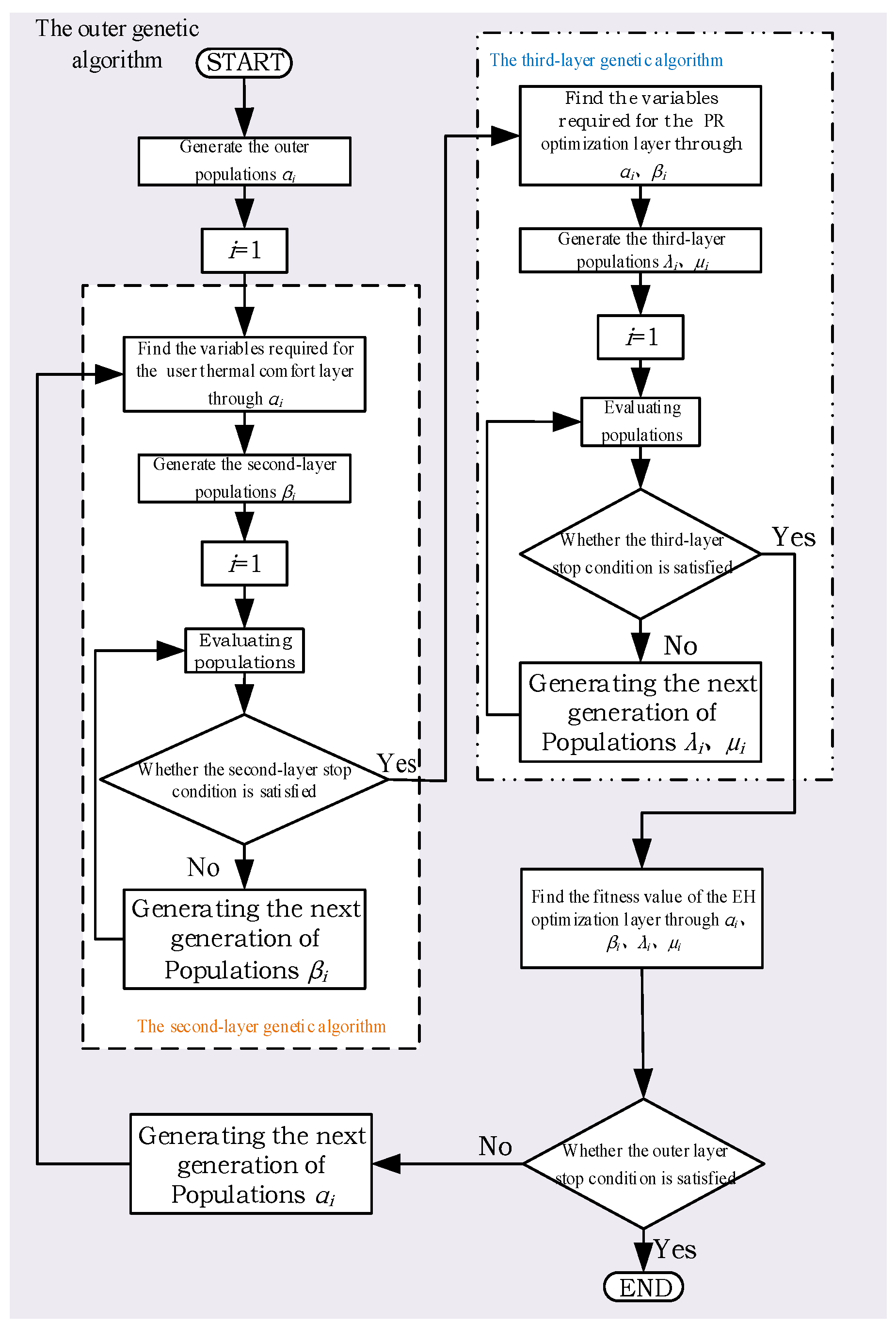
  • To solve the MOBO problem of the IEH, an improved multilayer nested quantum genetic algorithm is proposed. The algorithm has better performance and applicability for an IEH with a complex structure.

2. Structure of the IEH

Figure 1 shows the structure of the IEH, containing equipment such as a PR, CHP, a converter, and electric heater equipment. The PR contains an information layer and a physical layer. The information layer is mainly responsible for the exchange of information with the outer structure and the control and protection of the PR; the physical layer is mainly responsible for the conversion between AC power and DC power inside the PR.

2.1. Operation Strategy of the PR

Based on the structure of the PR used in this paper, the input–output matrix of this PR can be derived as
( P A P R P D P R ) = η P R ( g P R ( 1 λ ) μ g P R λ 1 μ ) ( P A P D )
where P A and P D are
{ P A = η P R ( P A + P E C H P ) ± P k A ( k = c , f ) P D = η P R P D ± P k D ( k = c , f )
Considering the uncertainty of renewable energy source supply, in order to fully utilize renewable energy sources and improve the efficiency of electric energy utilization, this study establishes the operation strategy of the PR under different operating conditions:
(1) Renewable energy sources provide power that can satisfy the demand of electrical load, i.e., η P R 2 PDLD + LA/(1 − β).
At this time, PA = 0. If the storage module is in charging mode, the charging power PcA is
{ P c A = P c max ( η P R P E C H P P c max ) P c A = η P R P E C H P ( P c min η P R P E C H P < P c max ) P c A = 0 ( η P R P E C H P < P c min )
The charging power PcD is
{ P c D = P c max ( η P R 2 P D ( L A 1 β + L D ) P c max ) P c D = η P R 2 P D ( L A 1 β + L D ) ( P c min η P R 2 P D ( L A 1 β + L D ) < P c max ) P c D = 0 ( η P R 2 P D ( L A 1 β + L D ) < P c min )
If the storage module is in discharge mode, the discharge power Pfi = Pfmin(i = A, D).
(2) The sum of the power provided by the renewable energy sources and the power provided by the CHP can satisfy the demand of electric load, i.e., η P R 2 (PD + gPR P E C H P ) ≥ LD + LA/(1 − β).
At this time, PA = 0. If the storage module is in charging mode, the charging power Pci is
{ P c A = P c max , P c D = 0 ( η P R P D < P c min ) P c A = 0 , P c D = P c max ( η P R P E C H P < P c min ) P c A = P c max , P c D = η P R P D ( P c min η P R P D < P c max ) P c A = η P R P E C H P , P c D = P c max ( P c min η P R P E C H P < P c max ) P c A = P c max , P c D = P c max ( η P R P D , η P R P E C H P P c max )
If the storage module is in discharge mode, the discharge power Pfi = Pfmin (i = A, D).
(3) The sum of the power provided by the renewable energy sources and the power provided by the CHP is not sufficient to satisfy the demand of electric load, i.e., η P R 2 (PD + gPR P E C H P ) < LD + LA/(1 − β).
At this time, if the storage module is in charging mode, the charging power Pci and PA are
{ P c A = P c max , P c D = 0 ( η P R P D < P c min ) P c A = 0 , P c D = P c max ( η P R ( P A + P E C H P ) < P c min ) P c A = P c max , P c D = η P R P D ( P c min η P R P D < P c max ) P c A = η P R ( P A + P E C H P ) , P c D = P c max   ( P c min η P R ( P A + P E C H P ) < P c max ) P c A = P c max , P c D = P c max ( η P R P D , η P R ( P A + P E C H P ) P c max )
P A [ ( L A 1 β + L D ) η P R 2 ( P D + g P R P E C H P ) + η P R ( g P R P c A + P c D ) ] / η P R 2 g P R
If the storage module is in discharge mode, the discharge power Pfi = Pfmax (i = A, D) and PA is
P A [ ( L A 1 β + L D ) η P R 2 ( P D + g P R P E C H P ) η P R ( g P R P f A + P f D ) ] / η P R 2 g P R

2.2. Energy Conversion Model

Based on the IEH structure and the PR operation strategy proposed above, the energy conversion matrix of this IEH can be established based on the equivalence of the cooling loads to the superposition of the thermal and electric loads:
( L Q L A L D ) = ( ( 1 α ) η G B + α η Q C H P β η e h 0 0 ( 1 β ) 0 0 0 1 ) ( P G P A P R P s e l l , A P D P R P s e l l , D )

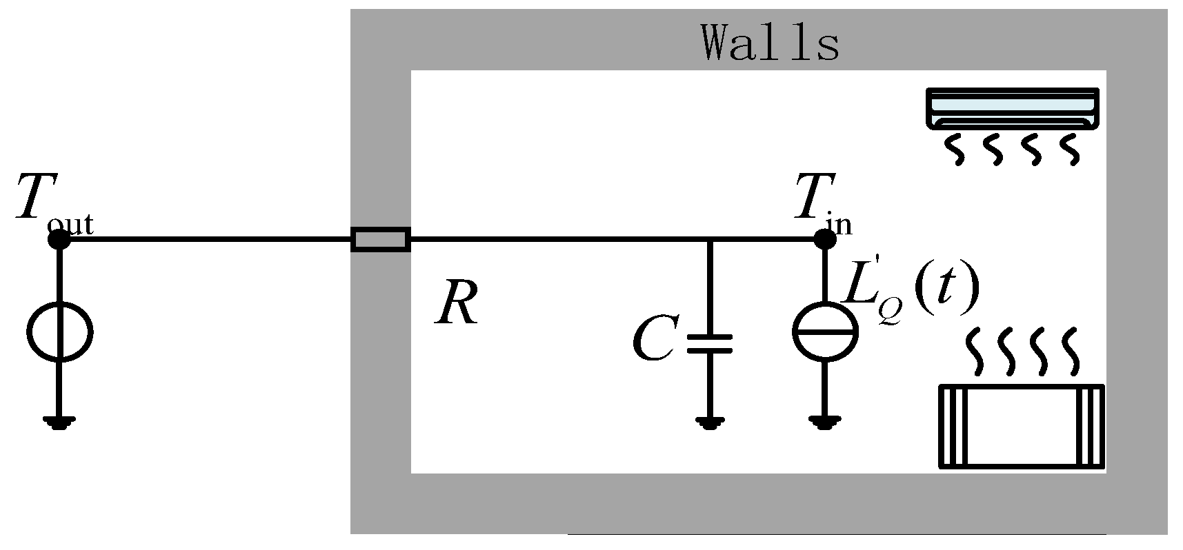
3. The Model of User Thermal Comfort

Currently, there are more studies on modeling related to human thermal comfort, including thermal sensory vote (TSV), standard effective temperature (SET), physiological equivalent temperature (PET), universal thermal climate index (UTCI), PMV value, etc. [26,27,28]. Since the TSV index mainly refers to the user’s subjective voting, the SET index does not consider “cold”, and the PET and the UTCI index are more focused on measuring thermal comfort in the outdoor area. In contrast, the PMV value developed by Fanger [29] and standardized in ASHRAE55 [30] establishes the relationship between the thermal load on the body and the statistical thermal sensation obtained from numerous people, which can better quantify the thermal comfort of the body indoors and has thus been adopted by the majority of studies. This study focuses on users’ indoor thermal comfort sensations. In summary, PMV values were chosen to model user thermal comfort in this study.
The PMV value is a comprehensive index used to evaluate the thermal comfort standard based on the equation of the human body’s heat balance state and considering human physiology, psychology, and other factors. The PMV value represents the average index of the population vote on seven levels of thermal sensation. A PMV value of 0 indicates moderate temperature, a PMV value of −1, −2, or −3 indicates slightly cool, cool, or cold, respectively, and a PMV value of +1, +2, or +3 indicates slightly warm, warm, or hot, respectively. The PMV value can be calculated using the following formula [31]:
V P M V = { 0.3895 ( T i n , t T 0 ) , T i n , t T 0 0.4065 ( T i n , t T 0 ) , T i n , t < T 0
where a PMV value between −1 and +1 is the comfort zone, and the corresponding indoor temperature is within the range of 23.54 °C and 28.57 °C. The closer the PMV value is to 0, the more comfortable the user is.
From Equation (10), it is clear that PMV values are mainly influenced by indoor temperature. Due to the thermal inertia of the building, the indoor temperature variation is mainly influenced by the heat load, outdoor temperature, and building parameters. The lumped-parameter equivalent model of the indoor temperature change process is shown in Appendix A, Figure A1.
The equation describing the indoor temperature change process can be obtained by listing the transient KCL equation for the equivalent model as
C d T in ( t ) d t = L Q ( t ) + T in ( t ) T o u t ( t ) R
The discretization is obtained by discretizing it:
T i n , t + 1 = T i n , t e Δ t τ + ( R L Q ( t ) + T o u t , t ) ( 1 e Δ t τ ) τ = R C
From Figure 1, the building heat load L Q ( t ) at time t consists of two parts: the output of the CHP and the output of the electric to thermal equipment, i.e.,
L Q ( t ) = P Q C H P ( t ) + ( β 1 β ) η e h L A ( t )
Therefore, the indoor temperature of the building at time t + 1 is
T i n , t + 1 = T i n , t e Δ t τ + [ R ( P Q C H P ( t ) + β 1 β η e h L A ( t ) ) + T o u t , t ] ( 1 e Δ t τ )

4. Optimization Model

The matrix form of the energy conversion model of the EH can be simplified as L = T(α,β)P; the input–output matrix of the PR can be simplified as PPR = T(λ,μ)P. Thus, the fundamental aim of the optimization model is to find the optimal conversion matrices T(α,β) and T(λ,μ).
When the EH is optimized, the EH can be optimized as a whole, which means that the coupling relationship of the internal devices does not need to be considered. Thus, the optimal matrix T can be easily found, whereas in the optimization of the IEH proposed in this paper, the outputs P A P R and P D P R of the PR need to be solved first. If the outputs P A P R and P D P R are wanted, the α and β parameters need to be determined. The β parameter is mainly determined by user thermal comfort. In the optimization, it can be seen that not only should the coupling relationship of each device in the IEH be considered, but also the influence of user behavior on it. Therefore, this study proposes a three-layer optimization model, which comprises a user thermal comfort layer, a PR optimization layer, and an EH optimization layer. The optimization model used is shown in Figure A2 in Appendix A.
In optimization, firstly, we generate n αi; secondly, the user thermal comfort layer calculates the optimal solution βi corresponding to αi based on the thermal load data and αi; afterward, the PR optimization layer uses n groups (αi, βi) to output the optimal solution (λi, μi) corresponding to each group (αi, βi) according to its objective function; lastly, the EH optimization layer calculates the optimal group (α, β, λ, μ) according to the n groups (αi, βi, λi, μi) outputted from the PR optimization layer.

4.1. User Thermal Comfort Layer

The user thermal comfort layer has the objective of satisfying user thermal comfort. Therefore, the objective function of the user thermal comfort layer is
min F ( β 2 ) = | V P M V ( L Q ( t ) , L A ( t ) ) |
where VPMV (LQ(t), LA(t)) is the user thermal comfort value at time t. After taking the absolute value of the thermal comfort value, its value domain is [0, +∞]; from the above, it can be seen that the thermal comfort value is closer to 0 the more comfortable the user is, so we took its minimum value.

4.2. EH Optimization Layer

The EH optimization layer aims to minimize the overall system operating costs. The system operating costs include the integrated operating cost C(t) and the pollutant emission cost P(t). The decision variables for this objective function are α and β.
min F ( α , β ) = t C ( t ) + t P ( t )
The integrated operating cost C(t) takes into account the cost of purchased energy C1 and the cost of energy substitution CDR, i.e., C = C1 + CDR.
C 1 ( t ) = P G ( t ) Q g a s φ t G + P A ( t ) φ t A
where the right side of the equation comprises the cost of purchased gas and the cost of purchased electricity, respectively.
C D R ( t ) = α P G ( t ) Q g a s φ t G ( η G B η Q C H P ) P E C H P ( t ) φ t A + β ( P A P R ( t ) P s e l l , A ) ( q t A q t Q )
where CDR(t) is the cost of energy substitution, including the cost of CHP heat and electricity substitution and the cost of electricity to heat.
P P ( t ) = P Q G B ( t ) C G B + P E C H P ( t ) C C H P + P A ( t ) C A + P D ( t ) C D

4.3. PR Optimization Layer

The PR optimization layer has the objective of maximizing the revenue of the PR. The PR revenue includes the cost of electricity sold Csell(t), the cost of batteries Cbat(t), and the cost of electricity purchased Cbuy(t). The decision variables are λ, μ, and PA(t). We define the objective function using:
max F ( λ , μ , P A ( t ) ) = y ( t )
where y(t) = Csell(t) − Cbat(t) − Cbuy(t). The objective function varies according to the operating conditions of the PR:
  • If the PR is in operating condition 1 or 2 at time t, then y(t) = Csell(t) − Cbat(t).
  • If the PR is in operating condition 3 at time t, then y(t) = Csell(t) − Cbat(t) − Cbuy(t).
The cost of electricity sold in the PR optimization layer Csell(t) is
C s e l l ( t ) = P s e l l . A ( t ) ν t A + P s e l l . D ( t ) ν t D
With reference to study [18] in the battery cost calculation method, the operating cost of battery t hours can be obtained as
C b a t ( t ) = | Δ W b a t ( t ) | C B 2 N × W B
where ΔWB(t) is the loss at the moment of tWbat(t) = ηbPci(i = A, D) in charging mode and ΔWbat(t) = Pci/ηb(i = A, D) in discharging mode). The charging and discharging states of the energy storage device are controllable when the charging and discharging constraints are satisfied.
The cost of power purchase Cbuy(t) in the PR optimization layer is
C b u y ( t ) = P A ( t ) φ t A

4.4. Constraints

(1) Charge/discharge constraints
The storage module charging and discharging power cannot exceed its minimum and maximum values, i.e.,
P c min P c i P c max
P f min P f i P f max
At the same time, the storage module can only run in one mode, i.e.,
P c i ( t ) P f i ( t ) = 0
At time t, the storage module charges Eci(t) = η Pbci(t) and discharges Efi(t) = Pfi(t)b.
(2) Charge state constraints
S O C min S O C S O C max
The energy storage capacity E(t) of the storage module at time t is satisfied:
E min E ( t ) E max
and the energy storage capacity E(t + 1) at time t + 1 is satisfied:
E ( t + 1 ) = E ( t ) + ( E c A ( t ) + E c D ( t ) ) ( E f A ( t ) + E f D ( t ) )
(3) Renewable energy constraints
In this study, for renewable energy generation, mainly photovoltaic power generation and wind power generation, there is only active power, and all of them are controlled by maximum power tracking. Their operating power constraints are
{ P p v min P p v P p v max P w t min P w t P w t max
(4) Energy network constraints
The minimum and maximum constraints for the CHP and gas boiler treatments are based on the unit characteristics, respectively:
{ 0 P E C H P P E . max C H P 0 P Q C H P P Q . max C H P
0 P Q G B P Q . max G B
In order to minimize the impact of IEHs on the regional grid, the electricity market specifies that power purchases must be within a certain range and also that power purchases need to satisfy the transmission capacity constraints of the equipment involved.
Similarly, the natural gas purchased from the natural gas grid and the electricity sold are also within a determined range and satisfy the transmission capacity constraints of the equipment.
{ 0 P A ( t ) P A max 0 P A ( t ) P A t max
{ 0 P G ( t ) P G max 0 P G ( t ) P G t max
{ 0 P s e l l . A P s e l l . A max 0 P s e l l . D P s e l l . D max

5. Algorithm Flow

This study proposes an improved multi-layer nested quantum genetic algorithm (IMNQGA) to solve this objective function, and the flow chart of the algorithm is shown in Figure 2. In this algorithm, the second-layer genetic algorithm aims to find the optimal β of the user thermal comfort layer; the third-layer genetic algorithm aims to find the optimal λ and μ of the PR optimization layer; and the outer genetic algorithm calculates the optimal solution of the EH optimization layer based on the values of β, λ, and μ obtained by the inner two-layer algorithm. These three layers of the genetic algorithm are articulated and corrected by the constraints and the internal logic of the model, and then the overall optimal solution is obtained.
In addition, the algorithm is a nesting of three layers of genetic algorithms, and the amount of computation and complexity is exponentially more that of an ordinary genetic algorithm. Therefore, in order to reduce the number of calculations and save time, we used the active detection stopping method. When the running cost of the EH optimization layer reaches a certain range or remains unchanged for a long time, it can be considered that the algorithm has found the optimal solution and stops the calculation [32].

6. Example Analysis

In this study, we selected the typical daily data of an apartment complex in Hebei Province during winter as the research object.
The heat loads, AC loads, DC loads, and renewable energy sources that provide power profiles for this apartment complex are shown in Figure 3.
The time-of-use electricity price and other parameter settings in the model were determined with reference to [18,33], and the specific values are shown in Table 1 and Table 2.
In order to verify the effectiveness of the model, four operational models were constructed for comparison as follows.
Mode 1: Considering user thermal comfort, the parameters α, β, λ, and μ are optimized once per operating period within 24 h using the IEH structure and applying the optimization model proposed in the paper.
Mode 2: Considering user thermal comfort, a conventional EH structure is used, and the structure is shown in Figure A3 in Appendix A. The matrix form of its energy conversion model is:
[ L Q L E ] = [ ( 1 α ) η G B + α η Q C H P + α β η E C H P β α ( 1 β ) η E C H P 1 β ] [ P G P E ]
where LE is the electrical load, which is the total load of the AC and DC, i.e., LE = LA + ηADLD; ηAD is the AC/DC load conversion factor; PE is the power provided by electricity, which is the total power provided by renewable energy sources when they are integrated into the AC grid, i.e., PE = PA + ηDAPD; and ηDA is the loss coefficient of renewable energy sources when they are integrated into the power grid.
Since the structure of Mode 2 does not contain the PR, the optimization model used in Mode 2 does not contain the PR optimization layer, i.e., the EH optimization layer optimizes the primary parameters α and β through the β output of the user thermal comfort layer for each operation period within the 24 h period.
Mode 3: User thermal comfort is not considered, i.e., β = 0, the optimization model does not include the user thermal comfort layer, and the parameters α, λ, and μ are optimized once for each operation period within 24 h, and the other settings are the same as in Mode 1.
Mode 4: On the basis of Mode 2, user thermal comfort is not considered, i.e., only the operating cost objective of the EH optimization layer needs to be considered in the optimization, and the parameter α is optimized once for each operating period within 24 h, and the other settings are the same as in Mode 2.
The algorithm proposed in this paper is used to solve the above four modes. The changes in the parameters of α, β, λ, and μ of the four modes within 24 h of optimization are shown in Figure 4. The PMV values and operating cost results obtained after optimization are shown in Figure 5 and Figure 6.
As can be seen in Figure 5 and Figure 6, the operating cost of the system with the IEH structure proposed in this paper is significantly reduced. After considering user thermal comfort, the system operating costs show a slight increase, but the PMV values can be overwhelmingly controlled in the range of [−1, 1] and mostly in the range of [−0.5, 0.5], which significantly improves user thermal comfort.
To further verify the validity and feasibility of the model proposed in this paper, the system energy-use efficiency metric Ef = (LQ + LA + LD)/(G + PA + PD), i.e., the ratio of total output to input, is defined. The results of the operation in the four modes are organized to obtain the energy-use efficiency curves for each mode, as shown in Figure 7.
In Figure 7, it can be seen that the energy-use efficiency of Mode 1 and Mode 3 is higher than that of Mode 2 and Mode 4, i.e., the adoption of the IEH structure proposed in this paper can enhance the energy-use efficiency of the system and promote the consumption of renewable energy, which is valuable for the study of enhancing the energy efficiency of the system for the utilization of multi-energy complementarity.
The total value of operating costs, the average value of energy-use efficiency, and the mean and standard deviation of user thermal comfort in the four models were further compared, and the results are shown in Figure 8 and Figure 9.
We combine Figure 5, Figure 6, Figure 7, Figure 8 and Figure 9 and compare the differences between the four mode shown. The following conclusions can be drawn. As shown in Table 3.
From this table, it can be seen that adopting the IEH structure proposed in this paper can reduce the system’s operating costs and improve the system’s energy-use efficiency; considering user thermal comfort will increase the system’s operating costs, but it can significantly improve user thermal comfort; and by considering user thermal comfort and adopting the IEH structure of the system compared with the conventional EH system that does not consider user thermal comfort, the operating costs can be reduced while keeping user thermal comfort within the comfortable range and improving the energy-use efficiency of the system.

7. Conclusions

This paper introduces user thermal comfort on the basis of the proposed IEH structure; provides an optimization model considering user thermal comfort, system operating costs, and PR revenue; and proposes an improved multi-layer nested quantum genetic algorithm to solve the problem. Finally, a real IES is used as an arithmetic example, which is verified using research results and historical operation data, and the main conclusions are as follows:
(1) The IEH structure replaces the electrical part of the conventional EH with the PR, which further enhances the multi-energy utilization efficiency of the EH, effectively promotes the consumption of renewable energy sources, reduces the system operating costs, and enhances the energy-use efficiency.
(2) The optimization control method proposed in this paper introduces user thermal comfort. From the analysis of other examples, it can be seen that user thermal comfort can be used to describe the thermal inertia problem of heat load and the behavior of heat users. The proposed method can balance user thermal comfort and the system operating costs, which significantly improves the user’s environmental quality.
In addition, although the IMQGA proposed in this study can effectively solve the optimization problem, it still suffers from the problems of long running time and a high number of iterations. Therefore, the direction of our future work is to investigate a more efficient algorithm applicable to IEHs.

Author Contributions

Conceptualization, H.Z.; writing—original draft preparation, K.Y.; writing—review and editing, H.Z. All authors have read and agreed to the published version of the manuscript.

Funding

This research was funded by the National Key Research and Development Program of China under Grant No. 2021YFB2400800, “Response-Driven Intelligent Enhancement Analysis and Control for Bulk Power System Stability”.

Data Availability Statement

Due to the nature of this research, participants of this study did not agree for their data to be shared publicly, so supporting data is not available.

Conflicts of Interest

The authors declare no conflict of interest.

Nomenclature

PGPurchased natural gas power (kW)
PAAC power (kW)
PDDC power supplied by renewable energy (kW)
LQHeat load (kW)
LAAC load (kW)
LDDC load (kW)
Psell,AAC power sold to the grid (kW)
Psell,DDC power sold to the grid (kW)
P A P R AC power output from the PR (kW)
P D P R DC power output from the PR (kW)
αRatio of natural gas power input to CHP to total natural gas power
βRatio of the electric power input to the electric heater equipment to the electric power remaining after the AC power output from the PR is sold to the grid
λRatio of electrical power input to the DC side after passing through a DC/DC converter
μRatio of electrical power input to the AC side after passing through the DC/DC converter
P E C H P Electrical power supplied by CHP (kW)
P Q C H P Thermal power provided by CHP (kW)
ηPREfficiency of PR conversion level
gPREfficiency of PR isolation level
ηehHeating efficiency of electric heater equipment
P A PA transformed through the storage module (kW)
P D PD transformed through the storage module (kW)
PcACharging power on the upper side of the storage module (kW)
PcDCharging power on the lower side of the storage module (kW)
PfADischarging power on the upper side of the storage module (kW)
PfDDischarging power on the lower side of the storage module (kW)
ηGBHeating efficiency of the gas boiler
η Q C H P Efficiency of natural gas converted to heat power through the CHP
Tin,tIndoor temperature of the building at time t (°C)
T0Indoor comfort temperature value; 26 °C is taken in this paper
L Q (t)Heat load of the building at the time t (kW)
CSpecific heat capacity of the building
RThermal resistance of the building
Tout,tOutdoor temperature of the building at the time t (°C)
τ Thermal inertia constant
φ t G Price of natural gas (CNY/kWh)
QgasLow calorific value of natural gas; 9.97 kWh/m3 is taken in this paper
φ t A Real-time price of ac electricity (CNY/kWh)
q t Q User-side unit heat price (CNY/kWh)
q t A User-side unit electricity price (CNY/kWh)
CGBCost of pollutant treatment for gas-fired boilers (CNY/kWh)
CCHPCost of pollutant treatment for CHP (CNY/kWh)
CACost of pollutant treatment for the production of ac electricity (CNY/kWh)
CDCost of pollutant treatment for renewable energy generation (CNY/kWh)
v t A Unit price of ac electricity sold (CNY/kWh)
v t D Unit price of dc electricity sold (CNY/kWh)
CBPrice of the battery pack (CNY)
WBRated capacity of the battery pack (kW)
NNumber of times the battery pack has been used for charging and discharging cycles
ηbCharging and discharging efficiency
PcminMinimal limit value of charging power (kW)
PfminMinimal limit value of discharging power (kW)
PcmaxMaximum limit value of charging power (kW)
PfmaxMaximum limit value of discharging power (kW)
SOCState of charge of storage module
SOCminMinimum state of charge of storage module
SOCmaxMaximum state of charge of storage module
PpvPV operating power (kW)
PwtWind turbine operating power (kW)
PpvminPV operating power minimum (kW)
PwtminWind turbine operating power minimum (kW)
PpvmaxPV operating power maximum (kW)
PwtmaxWind turbine operating power maximum (kW)
PAtmaxMaximum limit of transmission capacity of electric equipment (kW)
PGtmaxMaximum limit of transmission capacity of natural gas equipment (kW)
Psell.AtmaxMaximum limit of sold ac power (kW)
Psell.DtmaxMaximum limit of sold dc power (kW)

Appendix A

Figure A1. Equivalent model of temperature change process.
Energies 17 00948 g0a1
Figure A2. Three-layer optimization model.
Energies 17 00948 g0a2
Figure A3. The structure of normal EH.
Energies 17 00948 g0a3

Appendix B

Equation (1): The structure of PR in the IEH structure proposed in this paper is shown in the following figure.
Energies 17 00948 i001
As can be seen from the figure:
{ P A = η P R ( P A + P E C H P ) ± P k A   ( k = c , f ) P D = η P R P D ± P k D ( k = c , f )
Subsequently, PR can be simplified to:
Energies 17 00948 i002
It can be obtained eventually that
P A P R = η P R g P R ( 1 λ ) P A + η P R μ P D
P D P R = η P R g P R λ P A + η P R ( 1 μ ) P D
i.e., ( P A P R P D P R ) = η P R ( g P R ( 1 λ ) μ g P R λ 1 μ ) ( P A P D )
Equation (9): The IEH structure can be simplified as:
Energies 17 00948 i003
It can be obtained eventually that
L A = ( 1 β ) ( P A P R P s e l l . A )
L D = ( P D P R P s e l l . D )
L Q = ( 1 α ) η G B P G + α η Q C H P P G + β η e h ( P A P R P s e l l . A )
i.e., ( L Q L A L D ) = ( ( 1 α ) η G B + α η Q C H P β η e h 0 0 ( 1 β ) 0 0 0 1 ) ( P G P A P R P s e l l , A P D P R P s e l l , D ) .

References

  1. Cao, J.; Meng, K.; Wang, J.; Yang, M.; Chen, Z.; Li, W.; Lin, C. An energy internet and energy routers. Sci. China (Inf. Sci.) 2014, 44, 714–727. [Google Scholar]
  2. Yu, X.; Xu, X.; Chen, S.; Wu, J.; Jia, H. A brief review to IES and energy internet. Trans. China Electrotech. Soc. 2016, 31, 1–13. [Google Scholar]
  3. Geidl, M.; Andersson, G. Optimal power flow of multiple energy carriers. IEEE Trans. Power Syst. 2007, 22, 145–155. [Google Scholar] [CrossRef]
  4. Huang, Y.; Wu, S.; Xu, J.; Chen, J.; Yang, M.; Xie, J.; Zhang, D. Game Optimal scheduling among multiple EHs considering environmental cost with incomplete information. Autom. Electr. Power Syst. 2022, 46, 109–118. [Google Scholar]
  5. Xu, X.; Jia, H.; Jin, X.; Yu, X.; Mu, Y. Study on hybrid heat-gas-power flow algorithm for integrated community energy system. Proc. CSEE 2015, 35, 3634–3642. [Google Scholar]
  6. Chen, L.; Lin, X.; Xu, Y.; Li, T.; Lin, L.; Huang, C. Modeling and multi-objective optimal dispatch of micro energy grid based on EH. Power Syst. Prot. Control. 2019, 47, 9–16. [Google Scholar]
  7. Ma, T.; Wu, J.; Hao, L.; Li, Y. Energy flow modeling and optimal operation analysis of micro energy grid based on EH. Power Syst. Technol. 2018, 42, 179–186. [Google Scholar]
  8. Mokaramian, E.; Shayeghi, H.; Sedaghati, F.; Safari, A.; Alhelou, H.H. A C-VaR-robust-based multi-objective optimization model for EH considering uncertainty and e-fuel energy storage in energy and reserve markets. IEEE Access 2021, 9, 109447–109464. [Google Scholar] [CrossRef]
  9. Hu, J.; Liu, X.; Shahidehpour, M.; Xia, S. Optimal operation of EHs with large-scale distributed energy resources for distribution network congestion management. IEEE Trans. Sustain. Energy 2021, 12, 1755–1765. [Google Scholar] [CrossRef]
  10. Cheng, E.; Wei, Z.; Ji, W.; Ye, T.; Chen, S.; Zhou, Y.; Sun, G. Distributed optimization of integrated electricity-heat energy system considering multiple EHs. Electr. Power Autom. Equip. 2022, 42, 37–44. [Google Scholar]
  11. Yang, Y.; Li, J. Blockchain-based energy transaction model for multiple EHs. In Proceedings of the 2021 IEEE 10th Data Driven Control and Learning Systems Conference, Suzhou, China, 14–16 May 2021; pp. 1235–1240. [Google Scholar]
  12. Ni, W.; Lin, L.; Xiang, Y.; Liu, J.Y.; Yang, Y.F.; Zhang, W.T. Optimal gas-Electricity purchase model for EH system based on chance-constrained programming. Power Syst. Technol. 2018, 42, 2477–2487. [Google Scholar]
  13. Yang, L.; Li, X.; Sun, M.; Sun, C. Hybrid Policy-Based Reinforcement Learning of Adaptive Energy Management for the Energy Transmission-Constrained Island Group. IEEE Trans. Ind. Inform. 2023, 19, 10751–10762. [Google Scholar] [CrossRef]
  14. Tajalli, S.Z.; Mardaneh, M.; Taherian-Fard, E.; Izadian, A.; Kavousi-Fard, A.; Dabbaghjamanesh, M.; Niknam, T. DoS-Resilient Distributed Optimal Scheduling in a Fog Supporting IIoT-Based Smart Microgrid. IEEE Trans. Ind. Appl. 2020, 56, 2968–2977. [Google Scholar] [CrossRef]
  15. Amirioun, M.H.; Aminifar, F.; Lesani, H. Towards Proactive Scheduling of Microgrids Against Extreme Floods. IEEE Trans. Smart Grid 2018, 9, 3900–3902. [Google Scholar] [CrossRef]
  16. Huang, A.Q.; Crow, M.L.; Heydt, G.T.; Zheng, J.P.; Dale, S.J. The Future Renewable Electric Energy Delivery and Management (FREEDM) System: The Energy Internet. Proc. Proc. IEEE 2011, 99, 133–148. [Google Scholar] [CrossRef]
  17. GB/T 40097-2021; Functional Specifications and Technical Requirements of Energy Router. China Electricity Council: Beijing, China, 2021.
  18. Li, P.; Sheng, W.; Duan, Q.; Li, Z.; Zhu, C.; Zhang, X. A lyapunov optimization-based energy management strategy for EH with energy router. IEEE Trans. Smart Grid 2020, 11, 4860–4870. [Google Scholar] [CrossRef]
  19. Shi, X.; Xia, H. Interactive bilevel multi-objective decision making. J. Oper. Res. Soc. 1997, 48, 943–949. [Google Scholar] [CrossRef]
  20. Lv, Y.; Wan, Z. Linear bilevel multiobjective optimization problem: Penalty approach. J. Ind. Manag. Optim. 2019, 15, 1213–1223. [Google Scholar] [CrossRef]
  21. Ji, Y.; Ma, G.; Wei, J.; Dai, Y. A hybrid approach for uncertain multi-criteria bilevel programs with a supply chain competition application. Intell. Fuzzy Syst. 2017, 33, 2999–3008. [Google Scholar] [CrossRef]
  22. Pieume, C.O.; Marcotte, P.; Fotso, L.P.; Siarry, P. Solving Bilevel Linear Multiobjective Programming Problems. Am. J. Oper. Res. 2011, 1, 214–219. [Google Scholar] [CrossRef]
  23. Mejía-de-Dios, J.A.; Rodríguez-Molina, A.; Mezura-Montes, E. Multiobjective Bilevel Optimization: A Survey of the State-of-the-Art. IEEE Trans. Syst. Man Cybern. Syst. 2023, 53, 5478–5490. [Google Scholar] [CrossRef]
  24. Cai, X.; Sun, Q.; Li, Z.; Xiao, Y.; Mei, Y.; Zhang, Q.; Li, X. Cooperative Coevolution with Knowledge-Based Dynamic Variable Decomposition for Bilevel Multiobjective Optimization. IEEE Trans. Evol. Comput. 2022, 26, 1553–1565. [Google Scholar] [CrossRef]
  25. Wang, B.; Zhao, W.; Lin, S.; Ke, J.; Wu, H. Integrated energy management of highway service area based on improved multi-objective quantum genetic algorithm. Power Syst. Technol. 2022, 46, 1742–1751. [Google Scholar]
  26. Dong, Y.; Wang, Y.; Ni, C. Dispatch of a combined heat-power system considering elasticity with thermal comfort. Dispatch of a combined heat-power system considering elasticity with thermal comfort. Power Syst. Prot. Control. 2021, 49, 26–34. [Google Scholar]
  27. Wang, S.; Zhang, S.; Cheng, H.; Yuan, K.; Song, Y.; Han, F. Reliability indices and evaluation method of IES considering thermal comfort level of customers. Autom. Electr. Power Syst. 2023, 47, 86–95. [Google Scholar]
  28. Asghari, M.; Teimori, G.; Abbasinia, M.; Shakeri, F.; Tajik, R.; Ghannadzadeh, M.J.; Ghalhari, G.F. T-hermal discomfort analysis using UTCI and MEMI (PET and PMV) in outdoor environments: Case study of two climates in Iran (Arak & Bandar Abbas). Weather 2019, 74, 57–64. [Google Scholar]
  29. Fanger, P.O. Thermal Comfort: Analysis and Application in Environmental Engineering; McGraw-Hill: New York, NY, USA, 1972. [Google Scholar]
  30. ANSI/ASHARE Standard 55-2013; Thermal Environmental Conditions for Human Occupancy. ASHARE: Peachtree Corners, GA, USA, 2013.
  31. Yang, X.; Fu, G.; Liu, F.; Tian, Y.; Xu, Y.; Chai, Z. Potential Evaluation and Control Strategy of Air Conditioning Load Aggregation Response Considering Multiple Factors. Power Syst. Technol. 2022, 46, 699–708. [Google Scholar]
  32. Liu, C.; Yu, Z.; Yu, J.; Guo, L. A scheduling algorithm for distributed hybrid flow-shop production scheduling problem. Mod. Manuf. Eng. 2020, 27–35+12. [Google Scholar]
  33. Hao, R.; Ai, Q.; Zhu, Y.; Wu, H.; Liang, Z. Hierarchical optimal dispatch based on EH for regional IES. Electr. Power Autom. Equip. 2017, 37, 171–178. [Google Scholar]
Figure 1. The structure of the IEH.
Energies 17 00948 g001
Figure 2. The process of the IMNQGA.
Energies 17 00948 g002
Figure 3. Load and renewable energy power curves. (a) Load curves. (b) Renewable energy power curves.
Energies 17 00948 g003
Figure 4. Parameter change curves for the four modes. (a) Mode 1 parameters. (b) Mode 2 parameters. (c) Mode 3 parameters. (d) Mode 4 parameters.
Energies 17 00948 g004
Figure 5. Graph of operating cost results for the four modes.
Energies 17 00948 g005
Figure 6. Graph of PMV value results for the four modes.
Energies 17 00948 g006
Figure 7. Energy-use efficiency curve plot for the four modes.
Energies 17 00948 g007
Figure 8. Total operating costs and average value of energy-use efficiency for the four modes.
Energies 17 00948 g008
Figure 9. Distribution of PMV values for the four models.
Energies 17 00948 g009
Table 1. Time-of-use electricity price parameters.
Price of ElectricityTimeCNY/kWh
Time-sharing tariff1:00–5:00, 23:00–24:000.5
13:00–18:000.73
6:00–12:00, 19:00–22:001.21
Table 2. Parameter settings.
ParametersValueParametersValue
ηPR0.984CGB0.107 CNY/kWh
gPR0.968CCHP0.018 CNY/kWh
ηGB0.916CA0.197 CNY/kWh
ηeh0.45CD0.156 CNY/kWh
η Q C H P 0.897 P E m a x C H P 500 kW
η E C H P 0.36 P Q m a x C H P 500 kW
ηb0.9
Table 3. Comparison summary table of the operation results for the four modes.
√: Better Than; ×: Worse Than; ⚪: About the Same asMode 2Mode 3Mode 4
Mode 1Operating cost×
Energy-use efficiency
User thermal comfort
Mode 2Operating cost ××
Energy-use efficiency×
User thermal comfort
Mode 3Operating cost
Energy-use efficiency
User thermal comfort
Disclaimer/Publisher’s Note: The statements, opinions and data contained in all publications are solely those of the individual author(s) and contributor(s) and not of MDPI and/or the editor(s). MDPI and/or the editor(s) disclaim responsibility for any injury to people or property resulting from any ideas, methods, instructions or products referred to in the content.

