Article

Estimation of Solar Irradiance Using a Neural Network Based on the Combination of Sky Camera Images and Meteorological Data

Environmental Physics Department, HUN-REN Centre for Energy Research, 1121 Budapest, Hungary
*
Author to whom correspondence should be addressed.
Energies 2024, 17(2), 438; https://doi.org/10.3390/en17020438
Submission received: 30 November 2023 / Revised: 4 January 2024 / Accepted: 11 January 2024 / Published: 16 January 2024

Abstract

:
In recent years, with the growing proliferation of photovoltaics (PV), accurate nowcasting of PV power has emerged as a challenge. Global horizontal irradiance (GHI), which is a key factor influencing PV power, is known to be highly variable as it is determined by short-term meteorological phenomena, particularly cloud movement. Deep learning and computer vision techniques applied to all-sky imagery are demonstrated to be highly accurate nowcasting methods, as they encode crucial information about the sky’s state. While these methods utilize deep neural network models, such as Convolutional Neural Networks (CNN), and attain high levels of accuracy, the training of image-based deep learning models demands significant computational resources. In this work, we present a computationally economical estimation technique, based on a deep learning model. We utilize both all-sky imagery and meteorological data, however, information on the sky’s state is encoded as a feature vector extracted using traditional image processing methods. We introduce six all-sky image features utilizing detailed knowledge of meteorological and physical phenomena, significantly decreasing the amount of input data and model complexity. We investigate the accuracy of the determined global and diffuse radiation for different combinations of meteorological parameters. The model is evaluated using two years of measurements from an on-site all-sky camera and an adjacent meteorological station. Our findings demonstrate that the model provides comparable accuracy to CNN-based methods, yet at a significantly lower computational cost.

Graphical Abstract

1. Introduction

In the global effort to transition towards renewable energy sources, the utilization of photovoltaic (PV) systems has emerged as a key area for decarbonizing the energy sector. Consequently, PV sources are experiencing a surge in popularity; according to the International Energy Agency (IEA), the global cumulative PV capacity exceeded 1185 GWp in 2023 [1]. While PV production presents the potential for generating clean power, the volatility of this power source affected by atmospheric processes undermines the reliability of solar resources for power production. This variability has a profound impact on the power system, influencing its stability and affecting voltage conditions and power flow. To ensure a stable and reliable energy supply, accurate forecasting of PV power is essential.
The high variability of PV production is primarily due to it being affected by atmospheric phenomena. Multiple studies demonstrated that clouds have the greatest impact on irradiance reaching ground level [2,3]. The irregular and rapid movement of clouds can completely transform the sky within a few seconds, significantly altering photovoltaic production [4,5]. This variability complicates maintaining the balance between production and consumption and timely interventions in the power system, resulting in increased integration costs for PV [6].
Since radiation is influenced by both cloud movements and other atmospheric conditions, the most accurate forecasting models take both into account [7]. However, this requires continuous and accurate monitoring of atmospheric parameters and cloud cover, as well as integrating these two data streams into a common forecast model.
Cloud impact on irradiation is assessed using all-sky imagery and neural networks, such as Convolutional Neural Networks (CNN) and multi-modal models [8,9,10]. While image-based ANNs offer high accuracy, they demand substantial resources compared to alternatives like statistical time series analysis [11]. This necessitates the development of resource-efficient methodologies that, in addition to allowing the integration of various data sources, ensure adequate estimation accuracy.
In this paper, an ANN-based irradiation nowcasting method is presented that uses in the moment measurements for estimating solar irradiation. The model combines the advantages of traditional image processing algorithms and data-driven approaches. Instead of utilizing all-sky images, the state of the sky is characterized by a feature vector generated using traditional image processing. This reduces the amount of data processed and makes the method highly efficient while still considering essential information from all-sky imagery. Additionally, meteorological parameters and other ancillary data are incorporated into the estimation. The nowcasting is evaluated using more than 2 years of all-sky images and meteorological data in 1-min resolution, recorded at a ground station in Budapest, Hungary. Validation is conducted using global horizontal irradiance (GHI) and diffuse horizontal irradiance (DHI) measurements recorded at the same location. The main contributions of this work are as follows.
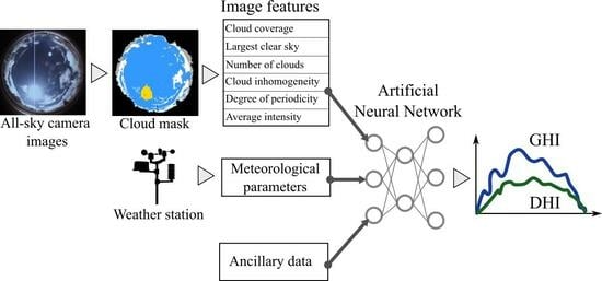
  • An ANN-based hybrid model is presented to estimate solar irradition parameters, using data sources of different modalities as an input, in particular all-sky imagery and meteorological data;
  • Six features characterizing sky conditions are introduced based on meteorological expertise. The features are obtained by means of traditional image processing from all-sky images. The advantages of this approach are two-fold: it incorporates crucial information about the condition of the sky, while it significantly decreases the amount of data used compared to image-based neural networks;
  • The impact of the different meteorological parameters on the estimation accuracy is investigated by comparing the performance of the model when different combinations of parameters are used as input.
Our main objective was to develop a nowcasting model to estimate irradiation by utilizing sky state and meteorological information. We aimed to understand the relationship between exogenous data and irradiation at a specific moment, providing crucial information about power generation at a specific location in the near future. This is essential for solar power plant operators to make real-time adjustments. Inference was performed for both GHI and DHI components, as these components influence PV power in different ways [12].
The rest of this paper is organized as follows. First, the remainder of the introduction presents related literature. Then, in Section 2 the proposed methodology is elaborated, including the measurement infrastructure (Section 2.1), the proposed image features obtained by traditional image processing (Section 2.2), the analyzed meteorological parameter combinations (Section 2.3), and the proposed ANN architecture (Section 2.4), respectively. In Section 3 evaluation results for the accuracy of the model are presented for the overall dataset as well as for various sky conditions. In Section 4 the discussion of modeling results are drawn, as well as the comparison with similar methods from the literature. In addition, the performance and complexity of the models are analyzed and compared to analogous CNN-based models from the literature. Finally, Section 5 concludes the article.

1.1. Related Works

Over the past decades, solar forecasting has predominantly focused on intra-day and day-ahead timeframes due to the limited resolution of available data [13]. However, the integration of PV production into the power system introduced a notable ramp rate from PV variability. This resulted in the demand for intra-hour or even intra-minute forecasting to enable real-time inverter control, active power curtailment, and dispatch operations [6,14]. Consequently, solar nowcasting, particularly ground-based approaches using sky observations, are crucial for power system control [15,16,17].
Solar ramp prediction necessitates exogenous inputs to the forecasting models, such as meteorological data and cloud cover information derived from all-sky images [18]. For this reason, in the intra-minute scale, sky-image-based techniques and time series forecasting using statistical models exhibit the highest, most robust forecasting capabilities [19,20]. Deep learning models, as an advanced version of statistical models, are gaining popularity due to their efficiency in handling the substantial amount of data from on-site sensors, cameras, and various databases [21]. Additionally, these methods inherently lend themselves to simultaneously processing multiple data sources, such as images, meteorological sensors, and ancillary data, which can be challenging to integrate otherwise.
Typically, fully connected neural networks are employed for processing weather data [15], while Long Short-Term Memory (LSTM) networks are utilized for forecasting, revealing patterns in short and long-term temporal correlations of cloud movement and solar irradiance [22]. For intra-minute analysis of cloud movement, the processing of all-sky camera imagery through image processing neural networks, such as CNNs [8,9,10] or Vision Transformer networks [23], is a popular approach. However, these techniques demand advanced computational infrastructure and a substantial amount of training data to achieve the desired accuracy, along with the drawback of a significant training time compared to other methods, such as statistical time series analysis [11].
Employing domain-reduction techniques can be beneficial to address these challenges. Hybrid solutions that use sky features as input to machine learning (ML) models are promising [9,24,25,26]. These solutions do not use raw images but rather features characterizing sky conditions. The simplest approach is to feed in the cloud cover besides other exogenous meteorological data to the model [25]. Cloud cover can be calculated using sky camera images [24] or obtained from another external source, i.e., online weather databases [25]. A more sophisticated approach utilizes various image features generated by a traditional image processing algorithm. Hu et al. [9] compute multiple features, including spectral, textural, cloud cover, and height features, as an ANN input to predict GHI in the ultra-short term. By using these features, the prediction accuracy measured in mean absolute percentage error has improved by 5% compared to the accuracy of the model without the feature information of ground-based cloud images. In a recent work, Terrén-Serrano et al. [26] use novel feature vectors that include previous clear sky index measurements, the position of the Sun, features describing cloud dynamics and statistics of these features; analyzing the best feature combination and their impact on accuracy when using various ML models. These features are based on an expert model, utilizing the information of the unique movement and dispersion of various cloud formations, reaching an accuracy of 54.64 W/m2 MAE (mean average error) for the support vector machine model for a forecasting horizon of 3 min.
As a result, combined methods require significantly less data during training, drastically reducing both training time and resource requirements. Although some information stored in the images may be lost, negatively impacting the method’s accuracy, this effect can be mitigated by selecting features representative of sky conditions.
In a study by Tsai et al. [27], the authors compared multiple GHI forecasting methods, including the hybrid nowcasting presented in Hu et al. [9]. The hybrid model taking cloud movement into account is shown to achieve comparable accuracy to other methods, as the mean average percentage error (MAPE) of the method was 7.8%, which is within the same order of magnitude as more complex methods, such as the CNN and LSTM combination network published in the study by Wang et al. in [28]. They achieved a 4% relative mean average error (rMAE), while its resource requirements remained very low. These findings highlight that the combination of machine learning and traditional image processing methods offers significant advantages in finding a balance between accuracy and resource requirements.

1.2. The Impact of Clouds on Irradiance

Technology-agnostic nowcasting usually aims to estimate GHI [5], which can subsequently be converted into PV power using parametric or nonparametric models [29]. In addition to GHI, DHI is also significantly affected by cloud dispersion and has a substantial impact on irradiance and, consequently, PV output [12]. It is recommended to analyze DHI separately from global radiation in photovoltaic production estimation applications.
DHI is primarily determined by the varying transmission and reflection capabilities of clouds. The sparsity in the transmittance of various clouds arises from differences in their micro- and macrophysical properties [3]. Determining this parameter is challenging because direct transmittance measurements are often unavailable for most clouds, as these clouds do not cast shadows on the utilized pyrheliometers. Nouri et al. [30] demonstrate a distinct correlation between low-layer optically thick clouds and high-layer optically thin clouds. However, middle-layer clouds exhibit ambiguity, displaying a significant dispersion ranging from optically thin to optically thick clouds.
Moreover, it is known, that dry air mass formations, airborne nanoparticles, and cloud formations can enhance the intensity of diffuse radiation also. The presence of fragmented clouds facilitates the focalization of sunlight and the occurrence of multiple reflection phenomena, leading to an elevation in both global and diffuse radiation levels, surpassing those observed in cloud-free conditions. The impact of clouds on radiative effect (RE)—whether attenuation or enhancement—largely depends on factors such as the extent of the cloud layer, the cloud’s position relative to the Sun, and specific cloud properties, including temperature and optical thickness. Experimental evidence indicates that global irradiance levels on flat surfaces can be raised by up to 40% due to the increased presence of diffuse radiation [12]. While these elevated levels may persist for only a few minutes, this phenomenon poses practical reliability challenges for photovoltaic applications. Therefore, as emphasized by Sánchez et al. [31], for this study, measurements and inference were performed for both direct and diffuse components.

2. Methodology

This section provides a detailed overview of the processing chain, encompassing data collection, image preprocessing, feature extraction from images, and the training and hyperparameter optimization of the applied ANN model.

2.1. Instrumentation and Measurement

Weather data and all-sky images are recorded by a measurement station located on rooftop of a building at the HUN-REN Center for Energy Research in Budapest (Latitude = 47.49225 N, Longitude = 18.953944 E). The station consists of a weather monitoring system and a total sky imager (TSI) (see Figure 1a). The TSI is a high-resolution, 180° wide-angle color Starlight Xpress Oculus all-sky camera, with its optical axis positioned vertically upwards. The camera captures images of the whole sky every minute (as shown in Figure 1b), with an image resolution of 370 × 370. For controlling the imaging process, custom software has been developed, so that the frequency of photography and exposure time can be adjusted. The imaging has been ongoing since November 2021, and since then the camera continuously records sky images during daylight hours.
The weather monitoring system is located in direct proximity to the camera capturing various meteorological parameters. It records the air temperature, surface wind speed, atmospheric pressure, and relative humidity, and solar irradiance (including GHI and DHI) using a pyranometer. These measurements are recorded at five-second intervals. The system logs one-minute average values and their corresponding one-minute standard deviations. Images and data are stored in a database for further processing. The system’s architecture is seen in Figure 1c.

2.2. Traditional Image Processing

2.2.1. Camera Calibration and Image Preprocessing

The images captured by the camera first undergo color correction, followed by the extraction of image features using color-channel thresholding. The raw images taken by the camera are preprocessed using multi-step color conversion. First, the color of a given pixel is calculated using demosaicing (also known as De-Bayer interpolation) in the RGB color space. Then, linear color conversion is applied to each color channel, the blue color channel is upscaled (scaling factor: 1.2), and the red color channel is downscaled (scaling factor: 0.95). Next, polynomial color conversion is applied. A conversion polynomial is empirically determined, subjecting the red, green, and blue color channels to luminance-dependent conversion. The last step is High Dynamic Range (HDR) merging of images with three different exposure times. HDR merging, a widely used technique for improving all-sky images [32] enhances contrast and reduces color saturation around the Sun region in the images. HDR merges images captured at different exposure times using the Mertens algorithm [33]. The preprocessing steps are illustrated in Figure 2.

2.2.2. All-Sky Image Segmentation

To extract cloud cover parameters from the sky images, the widely employed Red–Blue Ratio (RBR) cloud detection algorithm is used [34,35]. This method classifies the image pixels into cloud and clear sky regions, creating a binary image based on the values of the red and blue channels. For the classification, the following formula is employed:
I = R B
C = 1 , if I t h , 0 , otherwise ,
where R and B represent pixel values of the red and blue channel, respectively, I is the Red–Blue Ratio calculated for a specific pixel, and C constitutes the classification of the pixel in the binary image. t h is the threshold value determined through optimization. The resulting cloud mask for various sky conditions is seen in Figure 3.
The threshold was optimized using a self-developed reference database consisting of 120 sky images containing representative sky scenarios and cloud types. The database contains binary cloud masks for each all-sky image, representing the ideal segmentation result, and serving as a ground truth for the segmentation. The t h value was chosen to maximize both recall and accuracy of the RBR result across an empirically selected threshold range. The accuracy and recall of the various threshold setting is seen in Figure A1. The optimal threshold setting achieves an accuracy and recall of 85% across the representative dataset. Notably, it achieves even higher accuracy, reaching 94% with a recall of 91% for clear sky conditions. For cloudy sky conditions, the accuracy remains acceptable at 81% with a high recall at 95%. The algorithm has the lowest performance for partially cloudy sky conditions, with a recall and accuracy of 80%.
Oversaturated pixels in the Sun’s proximity can cause major classification problems for cloud detection. This is addressed using a twofold correction approach. First, saturated pixels in the circumsolar region are minimized by HDR merging as elaborated in Section 2.2.1. Second, an additional Sun mask is applied to the circumsolar region to filter out oversaturated pixels. The mask is created by selecting the largest saturated region and applying a flood fill algorithm to encompass all oversaturated pixels. The maximum saturation region obtained this way is subsequently masked for the remainder of the processing steps.
Similarly, a static mask was used to exclude surrounding objects in the image, using only the circular region in the middle for subsequent processing steps.
The resulting cloud mask is processed further to derive the image features utilized in the subsequent ANN inference, as explained in detail in the following section.
Image processing functionalities were implemented in C++ utilizing the OpenCV library [36].

2.2.3. Image Features

The main goal in designing features extracted from all-sky images for ANN inference was to identify features capable of encoding information about the impact of cloud formation on the measured irradiation.
Given the significant variability in transparency and light scattering among different cloud types, traditional cloud classification methods may not accurately estimate radiation-modifying effects due to the diverse impact of classical cloud types on radiation [30,37]. To address this limitation, we concentrated on defining cloud parameters that effectively characterize cloud types exhibiting similar behavior in terms of radiation modification. While several studies have explored automatic recognition of individual cloud types based on ground-based sky images [26,37,38,39], often utilizing more than 10 predefined parameter definitions for cloud classification, others, such as Zhang et al. [22], employed CNN for this purpose. While these studies demonstrated high accuracy in classifying individual clouds, challenges arose when dealing with scenarios involving multiple coexisting clouds. In contrast, our emphasis was not on precise cloud classification but rather on determining parameters relevant to the irradiance-modifying effects of cloud cover. The features are as follows:
  • Cloud coverage: The ratio of pixels covered by clouds to the total pixels in the image. GHI has a strong relationship with this parameter, but is not fully characterized by it. This parameter is the extension of the traditional octa-based cloud cover metric [3];
  • Largest clear sky area: The ratio of pixels of the largest contiguous clear sky area to the total pixels in the image. The time trend of the size of the clear sky could provide information about cloud drift;
  • Number of individual clouds: The number of contiguous cloud regions in the segmented image is a crucial factor in cloud type classification. It is also an important indicator of the temporal variability of radiation;
  • Cloud inhomogeneity: Proportion of thick cloud regions to the total cloud region. This parameter is extracted using Otsu’s method as described in Ref. [40], separating thick, dark clouds from thinner, white clouds. This parameter is characteristic of certain cloud types;
  • Degree of cloud periodicity: High periodicity is a characteristic feature of altocumulus clouds. This cloud genus exerts a substantial modifying impact on solar radiation, as detailed in Ref. [41], where it is noted that the most significant cloud radiative effect occurs when altocumulus clouds partially obscure the solar disk. The assessment of periodicity entails extracting an indicator through a 2D Fourier transform applied over the image domain. First, a frequency range is determined empirically, containing harmonic components typically seen in highly periodic cloud images. Then, the energy encoded by the components in the range relative to the total energy of the image is calculated. This feature discriminates against periodic altocumulus clouds (a typical sky condition characterized by altocumulus clouds is shown in Figure 4);
  • Average intensity: Average intensity of image pixels calculated across all three channels. This metric quantifies the overall radiance of the image, a parameter strongly correlated with GHI. However, this feature can be misleading thanks to the HDR merging performed on the images.
Figure 5 illustrates meteorological parameters and image features through the course of six selected sample days. The selected days encompass not only clear-sky scenarios but also instances of multiple cloud levels, including all different level type clouds as well as multi-level nimbusstratus. Recognizing the varying transmittance of irradiation and extent of different cloud types [30,39], we seek to emphasize the challenge of inferring global radiation solely from cloud coverage and highlighting a relationship between individual irradiation components and various sky conditions including multilevel and scattered clouds.
On day 10 March 2022, GHI closely follows the clear sky curve, with short periods of co-occurring medium and low-level clouds leading to highly variable temporal trends in global and diffuse irradiation.
On the second selected day (26 February 2023), besides the presence of morning stratocumulus clouds, the afternoon saw the overlay of altocumulus clouds, and high-level cirrostratus clouds were observed in the afternoon, followed by altocumulus clouds at sunset. The dominant diffuse component in irradiation indicated the prevalence of clouds in the sky.
On a clear day with passing clouds (20 June 2023), maintained predominantly clear skies. Only a brief appearance of high-level (cirrus) clouds around noon caused a decrease in GHI and an increase in the diffuse component due to the cloud radiative effect (CRE).
The fourth day (18 July 2023) showcased the movement of cumulus clouds alongside clear skies, leading to observable increases (enrichment) and decreases (ramp event) in irradiation throughout the day.
The morning of the fifth day (19 August 2023) featured a dense nimbostratus cloud, followed by the simultaneous appearance of high- and medium-level clouds. The dominance of the diffuse component suggested a significant contribution from CRE. Irradiation intensity varied throughout the day due to changes in cloud area and thickness, even when total cloud coverage remained relatively constant before noon.
On the sixth selected day (28 August 2023), persistent cloudiness of varying thickness prevailed, causing highly varying GHI dominated by diffuse irradiation.
These observations further underscore the significant influence of different cloud types on radiation and emphasize the need to separately evaluate different radiation components during estimation.
In Figure 6 the linear relationship between pairs of input and output data is quantified using the Pearson correlation coefficient. While GHI is highly correlated with temperature and cloud coverage, no single feature directly determines its intensity. On the other hand, DHI has a weaker relationship with each feature, except for cloud periodicity and cloud number, underscoring the complex relationship between cloud formation and irradiation.

2.3. Meteorological Scenarios

The analysis delves into the impact of individual meteorological measurements on global and diffuse radiation estimation accuracy.
The ANN model received as input the image features outlined in Section 2.2.2 as input data for each case. However, the weather station’s measured data (Table 1) were systematically selected, and multiple meteorological scenarios were formulated. When developing these scenarios, we focused on two key aspects: first, identifying the parameters essential for accurate radiation estimates, and second, assessing whether certain parameters, that do not possess additional information due to known physical laws (e.g., equation of state), can be excluded. The scenarios are detailed in Table 2.
The formulated weather scenarios are described in terms of their input data in Table 2. Different data combinations correspond to different scenarios. In Scenario 1, the meteorological parameters’ standard deviations are also incorporated. The clear sky (CSI) dataset is included only in the first two scenarios. The solar zenith angle (SZA) and image parameters (IF) are passed as inputs in all scenarios, along with the timestamp (DT) of the measurements. Further details regarding the measured quantities are provided in Table 1.
Additionally, a 6th scenario is designed, receiving only the basic meteorological parameters and no image features. This scenario is created as a benchmark for evaluating the impact of image features on the estimation accuracy.

2.4. Deep Neural Network

2.4.1. Data Processing

The various exogenous data types of estimation are detailed in Table 1. It contains three distinct data types: meteorological parameters recorded by the weather station, image features obtained from images captured by the sky camera, and additional ancillary data. Radiation values for a clear sky corresponding to the given geographical location, timestamps, and the solar zenith angle were used as ancillary data. Clear sky irradiation is the incident global radiation value estimated for a clear, cloudless sky for a given geographical location. A one-minute resolution McClear clear sky dataset was used for this purpose [42]. The solar zenith angle was also provided by the dataset. The data were compiled from measurements recorded between November 2021 and October 2023, comprising approximately 300,000 one-minute data points.
Temporal alignment was performed on images, weather data, and the clear sky dataset. This alignment considered the transition between daylight saving time and standard time, as well as the discrepancies between the weather measurements and images taken by different devices.
Erroneous measurement data, such as negative humidity values, were removed from the dataset. Only the part of the dataset corresponding to periods with sufficient irradiation (between 8 a.m. and 18 p.m.) was used. To achieve this, inappropriate data points were removed with the help of the weather station’s twilight sensor. The recording date and time were also added to the dataset as a timestamp. Time of day and day of year were converted into circular representation using two features, so that periods during the day and year close to each other are recognized as such.
To ensure balance in the input dataset, different GHI values were included with equal frequency among the input data. This was achieved by creating 10 equal histogram bins from the GHI values, and filtering the dataset so that each bin contained an equal number of sample points. However, due to the relative rarity of high irradiation samples, the top 5% of GHI values were omitted from the histogram equalization, and added without filtering to the input dataset. The resulting dataset was divided into training and validation sets in 80:20% ratio. The features of the training dataset were scaled to obtain a distribution with a mean of 0 and a standard deviation of 1 (standardization). The validation and test datasets were scaled accordingly to match the training data.

2.4.2. Network Architecture

A feed-forward multilayer perceptron deep neural network model was devised. The structure of the network is shown in Figure 7. Each network unit comprises three layers: a fully connected layer, a dropout layer, and a batch normalization layer. The fully connected layers have an identical number of neurons in each unit. Batch normalization and dropout were applied to each layer as a regularization technique preventing overfitting. The entire network was linked with the minute-by-minute GHI and DHI values, and training was conducted using the backpropagation method. The error during training was defined as the root mean square error (RMSE) of the difference between the estimated and measured irradiation, calculated for the sum of the two radiation components. The Adam optimizer [43] was chosen as the optimization algorithm due to its robust performance under various conditions. The software was written in Python, and experiments were conducted using the Tensorflow-Keras library [44].

2.4.3. Hyperparameter-Optimization

The model’s hyperparameters were fine-tuned for each scenario using Bayesian optimization [45]. The hyperparameters tuned included the activation function, the number of neurons in the fully connected layers, the number of fully connected layers, the dropout rate, and the learning rate of the Adam optimizer. The parameters and their value sets are summarized in Table 3. Hyperparameter value ranges were selected by empirical probing.
We defined a two-stage hyperparameter tuning process, that in the first stage explores various hyperparameter combinations using only a small part of the dataset. In the second stage, the model that achieved the best score in the initial phase undergoes further training using an expanded dataset.
During the first stage, we explored 75 different hyperparameter combinations for each weather scenario. Each combination was first trained for 15 epochs on a small dataset of 4000 randomly selected data points, split into training and validation sets in 80–20%. The score of the experiments was defined as the RMSE value obtained at the end of the trial. The top 20 trials by scenario are illustrated in Figure A2.
In the second stage, the model with the lowest score was further trained for additional 500 epochs using 100,000 data points. An early stopping of 50 epochs was used during this phase for further regularization. The epoch count and early stopping interval were empirically determined. This process results in the final network, which was used for evaluating the model performances. The best models’ hyperparameter values alongside their complexity are detailed in Table 4.
Based on the hyperparameter values of the top 20 models, it can be concluded that better scores could be achieved for scenario 1, the scenario utilizing the maximum number of meteorological parameters. Medium learning rates contribute to better scores in all scenarios, and networks perform optimally with either the gelu or the relu activation function. The number of layers of the best models is consistently 5, and it remains low, either 5 or 10 for the top 20 hyperparameter combinations, suggesting that a less complex network supports the problem complexity best.
The number of neurons per layer generally falls into the lower values, such as 128 or 256. An exception is scenario 5, with a layer size of 512. The complexity of the best network models, in addition to the size and layer count, is characterized by the number of weights and the network’s Million Floating-Point Instructions Per Second (MFLOPS) value in Table 4. It should be noted that the network for scenario 5 is an order of magnitude larger than the others. Since the network size characterizes the complexity of the inference problem of each scenario, this suggests that the network in scenario 5 deduces certain physical relationships between meteorological parameters that are implicitly contained in other weather parameters. Particularly, while the network for scenario 5 attains the lowest score during hyperparameter optimization, it performs the best on the test dataset consisting of solely unseen data (see Section 3). This is likely attributed to the complex structure of the network.

2.5. Evaluation Metrics

The accuracy of the estimation is quantified by scenario using the following four error metrics.
  • Root Mean Square Error:
    RMSE = i = 1 N ( y i y i ^ ) 2 N
  • Mean Bias Error:
    MBE = 1 N i = 1 N y i y i ^
  • Mean Absolute Percentage Error:
    MAPE = 1 N i = 1 N | y i y i ^ | y i
  • The coefficient of determination:
    R 2 = i = 1 N ( y i y ¯ ) 2 ( y i ^ y ¯ ^ ) 2 i = 1 N ( y i y ¯ ) 2 i = 1 N ( y i ^ y ¯ ^ ) 2 ,
    where y i ^ is the inferred value (GHI or DHI) and y i denotes the measured value at time step i. y ¯ and y ¯ ^ denotes the mean of estimates and measurements across all time steps and N denotes the number of samples the error is calculated for.

3. Results

The accuracy was also assessed for a dataset comprising all available samples, a total of 30,000 data points. Estimation accuracy is quantitatively evaluated using error metrics as defined in Section 2.5, and the results are seen in Table 5 and depicted in Figure 8. Notably, scenario 6, which excludes image features, exhibits significantly lower estimation accuracy compared to other scenarios that leverage image features, demonstrating a 20% decrease in MAPE compared to the best-performing scenario (scenario 5) for both GHI and DHI. Scenario 5 consistently outperforms all other scenarios, implying that a network with higher complexity performs better for the overall dataset.
The accuracy was further evaluated using an independent test dataset, comprising a total of 152,000 data points. This dataset included all samples not used during the training or hyperparameter optimization stages and was not part of the training or validation datasets. The results are shown in Table 6 and Figure 9. The results indicate that the error, both for GHI and DHI, is minimized in scenario 5, where MAPE is 17% for DHI and 21% for DHI, respectively. This outcome suggests that meteorological parameters have less impact on accuracy than image features, as scenario 5 uses the least meteorological data. The observed accuracy can also be attributed to the complexity of the model, as detailed in Section 2.4.3.
Scenarios incorporating image features consistently outperform scenario 6, demonstrating a 9% reduction in GHI MAPE and an 8% reduction in DHI MAPE compared to the best-performing scenario (scenario 5). An exception is scenario 3, which shows error rates comparable to scenario 6, indicating that this specific combination of meteorological parameters might negatively impact estimation accuracy.

4. Discussion

4.1. Accuracy for Selected Days

In our analysis, we also evaluate results based on cloud cover types, drawing insights from observations on the six sample days described in Section 2.2.2 to assess the model’s accuracy across diverse sky conditions. The comparison between measured and estimated GHI and DHI during the day is depicted in Figure 10, while Figure 11 quantifies the error metrics for the selected days. Additionally, Figure 12 showcases the correlation for these days for both irradiation components.
On the first day (10 March 2022), both medium and low-level clouds were detected. All models except scenario 6 excel in capturing these trends, demonstrating high accuracy even at a one-minute time resolution.
For the second day (26 February 2023), our model provided the most accurate estimate of DHI, showcasing its capability in handling variable cloud cover which was observable throughout the day.
On the third selected day (20 June 2023), with a clear sky and a brief appearance of cirrus clouds, the model demonstrates exceptional accuracy in clear-sky estimation and proficiently captures the radiation-modifying impact of high-level clouds, however not significantly pronounced.
On the fourth day (18 July 2022), the model’s limitations become evident, particularly in its ability to estimate unexpected increases and decreases. The accuracy of diffuse irradiance estimates due to the same phenomenon is only moderate.
The fifth day (19 August 2023) marked the most significant improvement across all scenarios compared to estimates without using parameters determined from image processing (scenario 6).
On the sixth selected day (28 August 2023) with persistent cloudiness, the model adeptly tracks temporal cloud inhomogeneity, showcasing excellent accuracy in estimating radiation changes attributable to cloudiness. However, precision diminishes slightly when addressing the appearance of cirrostratus clouds during midday when ramp events are detected.
It can be inferred that the hybrid model outlined in this study is capable of discerning these relationships, as it successfully identified changes in all studied cloud types, albeit with a slight underestimation, particularly in the case of cumulus clouds.
To account for these events, further development will focus on examining the spatial relationship of clouds and the Sun, as highlighted in the literature. As an illustration, Kazanatzidis et al. [39] conducted an extensive analysis, exploring the correlation between cloud types and their positions relative to the Sun, utilizing data obtained from a sky imager. Their study placed significant emphasis on the critical task of identifying and categorizing instances of scattered cloud cover, with a specific focus on situations where the solar disk is obstructed by clouds, as also emphasized in Ref. [41]. The relative positioning of the Sun and clouds in the sky emerged as a crucial factor in accurately estimating surface irradiance during enhancement events. According to their findings, for two specific cloud types, cirrus, and cumulus, the most significant enhancements occur when the clouds are close to the Sun and positioned in the upper portion of the sky, while the Sun occupies a lower position. Moreover, they demonstrated that the adverse impact of cloud cover on global radiation varies significantly for these types of clouds, resulting in substantial deviations in measured CRE values.

4.2. Comparative Analysis: Benchmarking against Existing Methods

This section compares the proposed method with other solar irradiation estimation methods in the literature, also focusing on the impact of selected parameters on estimation accuracy and computational resource requirements.
Comparison results are quantified in detail in Table 7.
In their exhaustive review, Zhang et al. [46] explore various GHI estimation models. High-time-resolution models in this study use a combination of mesoscale meteorological models and regression. Our study represents a significant advancement in GHI estimation accuracy, as the results show lower RMSE values (27.54 W/m2 to 89.33 W/m2) compared to the reviewed studies (88.33 W/m2 to 142.22 W/m2). The MBE error metric is also notably smaller in our case (refer to Table 7).
In a recent study, Alskaif et al. [47] identify meteorological variables impacting PV output power using high-resolution meteorological data. Examining five machine-learning-based regression models, the study concludes that a reduced number of meteorological variables ( n = 4 ) produces comparable results without affecting performance. Our study aligns with these findings, showing satisfactory accuracy with only a few well-selected meteorological parameters, especially when combined with sky image features in scenario 5. Ref. [47] also underscores the climate and area-dependent nature of solar irradiance estimation. Our results indicate a modest increase in the relative Mean Absolute Error (rMAE) range (0.1 to 0.17) compared to Ref. [47] (0.068 to 0.12). The relative Root Mean Square Error (rRMSE) is similar, ranging 0.16 to 0.23 compared to 0.1 to 0.15. A slight enhancement is noted in relative Mean Bias Error (rMBE), particularly in scenarios 1, 2, and 6, where the metric is 0.00 to 0.02 in our case. Additionally, it is crucial to note that metrics in [47] were calculated hourly, not minutely as in our study. Achieving these results at a higher time resolution is considered very positive, as higher resolution often leads to lower estimation accuracy especially under rapidly changing sky conditions as emphasized in Ref. [49].
Berrizbeitia et al. [48] provided an extended review of regression models of DHI to GHI ratio vs. clearness index, showing latitude-dependent results with R 2 = 0.80 to 0.87 for monthly averaged hourly DHI. In our study, a significant improvement in the DHI estimate was found as R 2 exceeded 0.87 for 1-min average DHI for all scenarios except scenario 6, which lacked image data and resulted in a slightly lower R 2 (0.76).
These findings consistently underscore that high-time-resolution solar irradiance estimation necessitates the constant monitoring of the sky incorporating images.
To assess the model’s resource efficiency, we compared its complexity, training time, and computational resource usage with two analogous CNN-based approaches, also taking estimation accuracy into account.
The first selected study by Papatheofanous et al. focuses on a CNN-based nowcasting model designed for real-time PV park control, with an emphasis on porting to Field-Programmable Gate Arrays (FPGA) [50]. This study employs various CNN models, including ResNet50 and SqueezeNet, quantized for FPGA operation to enable real-time efficiency. These models provide a benchmark for comparison with efficient models.
The second paper by Sansine et al. introduces a method for predicting GHI mean values one hour in advance, utilizing a multimodal network incorporating sky images and meteorological data [51]. Various deep learning models, including MLP, CNN, LSTM, and hybrids, are investigated, with the hybrid CNN-LSTM model emerging as the most accurate over a year’s worth of data. This paper serves as a suitable basis for comparison, as it combines image and meteorological data and utilizes a CNN model.
Our model is compared with these approaches based on trainable parameter count, Million Operations per Second (MOPS), and also accuracy using RMSE and MAE metrics. In the case of Ref. [50], quantized models use integer operations, while non-quantized models and the model presented in this study use floating-point operations. Ref. [51] lacks information on operations per second. The detailed performance comparison is presented in Table 8. Our hybrid model demonstrates the lowest parameter count and MOPS across all examined models. The exception is the MLP model in Ref. [51], which solely utilizes meteorological data and exhibits low training time and complexity but consequently achieves significantly lower accuracy. Despite the reduced parameter count, our model demonstrates error rates comparable to other models, proving to be an efficient tool for estimation.

5. Conclusions

This paper presents an ANN-based method for solar irradiance estimation, proposing a hybrid approach that combines traditional image processing with data-driven techniques. Instead of using all-sky camera images directly, a feature vector obtained by traditional image processing characterizes the sky’s state, enhancing computational efficiency. The model integrates meteorological parameters and ancillary data for improved estimation accuracy. The methodology was evaluated using over 2 years of 1-minute resolution all-sky images and meteorological data from Budapest, Hungary, with validation against GHI and DHI measurements at the same location. The impact of meteorological parameter combinations on estimation accuracy was also investigated.
The findings underscore the role of image features in estimation accuracy, as scenario 6, which excludes image features, exhibited a significant (20%) increase in MAPE compared to the best-performing scenario (scenario 5) when evaluated for a dataset containing a total of 300,000 samples. For an independent test dataset, scenario 5 consistently outperformed others, achieving a MAPE of 21% and 17% and R 2 of 0.96 and 0.98 for GHI and DHI, respectively. This suggests that apart from the utilization of image features the model’s complexity plays a significant role in achieving high-accuracy results for unseen circumstances. The findings suggest that two well-selected meteorological parameters (temperature and pressure) combined with parameters extracted from sky images can produce results with satisfactory accuracy.
The primary limitation of the approach is its location specificity, necessitating retraining for use in different climates. The model adaptation would require collecting meteorological measurements and whole-sky imagery for a representative period at the area of study, followed by obtaining the image features and training the neural network for that specific location, which can be a time-intensive process.
The methodology presented in this paper proves effective in inferring complex relationships between different sky conditions and their impact on solar irradiation. The model’s performance, especially in accurately estimating irradiance during enhancement events, positions it as a valuable tool for solar irradiance nowcasting. Future research will focus on accurately estimating ramp events, utilizing the relative position of the Sun and clouds. This method presents potential benefits for PV system operators by optimizing sensor selection for meteorological parameter measurement and improving overall computational efficiency.

Author Contributions

Conceptualization, L.B., V.G., and B.H.; methodology, L.B., D.G., and V.G.; software, L.B. and D.G.; validation, L.B. and D.G.; formal analysis, L.B., V.G., and D.G.; investigation, L.B., V.G. and D.G.; resources, B.H.; data curation, L.B. and D.G.; writing—original draft preparation, L.B.; writing—review and editing, L.B. and V.G.; visualization, L.B.; supervision, B.H. and J.O.; project administration, J.O.; funding acquisition, B.H. All authors have read and agreed to the published version of the manuscript.

Funding

This research received no external funding. The APC was funded by HUN-REN Centre for Energy Research.

Data Availability Statement

The data presented in this study are available on request from the corresponding author. The data are not publicly available due to privacy restrictions.

Acknowledgments

Supported by the ÚNKP-23-3-II-BME-280 New National Excellence Program of the Ministry for Culture and Innovation from the source of National Research, Development and Innovation Fund.

Conflicts of Interest

The authors declare no conflict of interest.

Appendix A

Figure A1. Accuracy and recall of the Red–Blue Ratio algorithm for various sky conditions.
Energies 17 00438 g0a1

Appendix B

Figure A2. The top 20 trials by scenario.
Energies 17 00438 g0a2

References

  1. Snapshot of Global PV Markets 2023. 2023. Available online: https://iea-pvps.org/snapshot-reports/snapshot-2023/ (accessed on 12 November 2023).
  2. Werner, M.; Ehrhard, R. Incident Solar Radiation over Europe Estimated from METEOSAT Data. J. Appl. Meteorol. Climatol. 1984, 23, 166–170. [Google Scholar] [CrossRef]
  3. Matuszko, D. Influence of the extent and genera of cloud cover on solar radiation intensity. Int. J. Climatol. 2012, 32, 2403–2414. [Google Scholar] [CrossRef]
  4. Jewell, W.; Ramakumar, R. The Effects of Moving Clouds on Electric Utilities with Dispersed Photovoltaic Generation. IEEE Trans. Energy Convers. 1987, EC-2, 570–576. [Google Scholar] [CrossRef]
  5. Barbieri, F.; Rajakaruna, S.; Ghosh, A. Very short-term photovoltaic power forecasting with cloud modeling: A review. Renew. Sustain. Energy Rev. 2017, 75, 242–263. [Google Scholar] [CrossRef]
  6. Samu, R.; Calais, M.; Shafiullah, G.; Moghbel, M.; Shoeb, M.A.; Nouri, B.; Blum, N. Applications for solar irradiance nowcasting in the control of microgrids: A review. Renew. Sustain. Energy Rev. 2021, 147, 111–187. [Google Scholar] [CrossRef]
  7. Mellit, A.; Massi Pavan, A.; Ogliari, E.; Leva, S.; Lughi, V. Advanced methods for photovoltaic output power forecasting: A review. Appl. Sci. 2020, 10, 487. [Google Scholar] [CrossRef]
  8. Li, Z.; Wang, K.; Li, C.; Zhao, M.; Cao, J. Multimodal Deep Learning for Solar Irradiance Prediction. In Proceedings of the 2019 International Conference on Internet of Things (iThings) and IEEE Green Computing and Communications (GreenCom) and IEEE Cyber, Physical and Social Computing (CPSCom) and IEEE Smart Data (SmartData), Atlanta, GA, USA, 14–17 July 2019; pp. 784–792. [Google Scholar] [CrossRef]
  9. Hu, K.; Wang, L.; Li, W.; Cao, S.; Shen, Y. Forecasting of solar radiation in photovoltaic power station based on ground-based cloud images and BP neural network. IET Gener. Transm. Distrib. 2022, 16, 333–350. [Google Scholar] [CrossRef]
  10. Feng, C.; Zhang, J.; Zhang, W.; Hodge, B.M. Convolutional neural networks for intra-hour solar forecasting based on sky image sequences. Appl. Energy 2022, 310, 118438. [Google Scholar] [CrossRef]
  11. Ahmed, R.; Sreeram, V.; Mishra, Y.; Arif, M. A review and evaluation of the state-of-the-art in PV solar power forecasting: Techniques and optimization. Renew. Sustain. Energy Rev. 2020, 124, 109792. [Google Scholar] [CrossRef]
  12. Balafas, C.; Athanassopoulou, M.; Argyropoulos, T.; Skafidas, P.; Dervos, C. Effect of the diffuse solar radiation on photovoltaic inverter output. In Proceedings of the Melecon 2010—2010 15th IEEE Mediterranean Electrotechnical Conference, Valletta, Malta, 26–28 April 2010; pp. 58–63. [Google Scholar] [CrossRef]
  13. Diagne, M.; David, M.; Lauret, P.; Boland, J.; Schmutz, N. Review of solar irradiance forecasting methods and a proposition for small-scale insular grids. Renew. Sustain. Energy Rev. 2013, 27, 65–76. [Google Scholar] [CrossRef]
  14. Ahmed, A.; Khalid, M. A review on the selected applications of forecasting models in renewable power systems. Renew. Sustain. Energy Rev. 2019, 100, 9–21. [Google Scholar] [CrossRef]
  15. Chu, Y.; Pedro, H.T.; Li, M.; Coimbra, C.F. Real-time forecasting of solar irradiance ramps with smart image processing. Sol. Energy 2015, 114, 91–104. [Google Scholar] [CrossRef]
  16. Saleh, M.; Meek, L.; Masoum, M.A.; Abshar, M. Battery-less short-term smoothing of photovoltaic generation using sky camera. IEEE Trans. Ind. Inform. 2017, 14, 403–414. [Google Scholar] [CrossRef]
  17. Wen, H.; Du, Y.; Chen, X.; Lim, E.; Wen, H.; Jiang, L.; Xiang, W. Deep learning based multistep solar forecasting for PV ramp-rate control using sky images. IEEE Trans. Ind. Inform. 2020, 17, 1397–1406. [Google Scholar] [CrossRef]
  18. Marquez, R.; Coimbra, C.F. Intra-hour DNI forecasting based on cloud tracking image analysis. Sol. Energy 2013, 91, 327–336. [Google Scholar] [CrossRef]
  19. Caldas, M.; Alonso-Suárez, R. Very short-term solar irradiance forecast using all-sky imaging and real-time irradiance measurements. Renew. Energy 2019, 143, 1643–1658. [Google Scholar] [CrossRef]
  20. Rajagukguk, R.A.; Ramadhan, R.A.A.; Lee, H.J. A Review on Deep Learning Models for Forecasting Time Series Data of Solar Irradiance and Photovoltaic Power. Energies 2020, 13, 6623. [Google Scholar] [CrossRef]
  21. Kumari, P.; Toshniwal, D. Deep learning models for solar irradiance forecasting: A comprehensive review. J. Clean. Prod. 2021, 318, 128566. [Google Scholar] [CrossRef]
  22. Zhang, J.; Liu, P.; Zhang, F.; Song, Q. CloudNet: Ground-based cloud classification with deep convolutional neural network. Geophys. Res. Lett. 2018, 45, 8665–8672. [Google Scholar] [CrossRef]
  23. Lin, Y.; Duan, D.; Hong, X.; Han, X.; Cheng, X.; Yang, L.; Cui, S. Transfer learning on the feature extractions of sky images for solar power production. In Proceedings of the 2019 IEEE Power & Energy Society General Meeting (PESGM), Atlanta, GA, USA, 4–8 August 2019; pp. 1–5. [Google Scholar]
  24. Chu, Y.; Coimbra, C.F. Short-term probabilistic forecasts for direct normal irradiance. Renew. Energy 2017, 101, 526–536. [Google Scholar] [CrossRef]
  25. Hosseini, M.; Katragadda, S.; Wojtkiewicz, J.; Gottumukkala, R.; Maida, A.; Chambers, T.L. Direct Normal Irradiance Forecasting Using Multivariate Gated Recurrent Units. Energies 2020, 13, 3914. [Google Scholar] [CrossRef]
  26. Terrén-Serrano, G.; Martínez-Ramón, M. Kernel learning for intra-hour solar forecasting with infrared sky images and cloud dynamic feature extraction. Renew. Sustain. Energy Rev. 2023, 175, 113125. [Google Scholar] [CrossRef]
  27. Tsai, W.C.; Tu, C.S.; Hong, C.M.; Lin, W.M. A Review of State-of-the-Art and Short-Term Forecasting Models for Solar PV Power Generation. Energies 2023, 16, 5436. [Google Scholar] [CrossRef]
  28. Wang, F.; Li, J.; Zhen, Z.; Wang, C.; Ren, H.; Ma, H.; Zhang, W.; Huang, L. Cloud Feature Extraction and Fluctuation Pattern Recognition Based Ultrashort-Term Regional PV Power Forecasting. IEEE Trans. Ind. Appl. 2022, 58, 6752–6767. [Google Scholar] [CrossRef]
  29. Almeida, M.P.; Muñoz, M.; de la Parra, I.; Perpiñán, O. Comparative study of PV power forecast using parametric and nonparametric PV models. Sol. Energy 2017, 155, 854–866. [Google Scholar] [CrossRef]
  30. Nouri, B.; Wilbert, S.; Segura, L.; Kuhn, P.; Hanrieder, N.; Kazantzidis, A.; Schmidt, T.; Zarzalejo, L.; Blanc, P.; Pitz-Paal, R. Determination of cloud transmittance for all sky imager based solar nowcasting. Sol. Energy 2019, 181, 251–263. [Google Scholar] [CrossRef]
  31. Sánchez, G.; Serrano, A.; Cancillo, M. Effect of cloudiness on solar global, solar diffuse and terrestrial downward radiation at Badajoz (Southwestern Spain). Opt. Pura Apl. 2012, 45, 33–38. [Google Scholar] [CrossRef]
  32. C. Valdelomar, P.; Gómez-Amo, J.L.; Peris-Ferrús, C.; Scarlatti, F.; Utrillas, M.P. Feasibility of ground-based sky-camera HDR imagery to determine solar irradiance and sky radiance over different geometries and sky conditions. Remote Sens. 2021, 13, 5157. [Google Scholar] [CrossRef]
  33. Mertens, T.; Kautz, J.; Van Reeth, F. Exposure Fusion. In Proceedings of the 15th Pacific Conference on Computer Graphics and Applications (PG’07), Maui, HI, USA, 29 October–2 November 2007; pp. 382–390. [Google Scholar] [CrossRef]
  34. Juncklaus Martins, B.; Cerentini, A.; Mantelli, S.L.; Loureiro Chaves, T.Z.; Moreira Branco, N.; von Wangenheim, A.; Rüther, R.; Marian Arrais, J. Systematic review of nowcasting approaches for solar energy production based upon ground-based cloud imaging. Sol. Energy Adv. 2022, 2, 100019. [Google Scholar] [CrossRef]
  35. Chow, C.W.; Urquhart, B.; Lave, M.; Dominguez, A.; Kleissl, J.; Shields, J.; Washom, B. Intra-hour forecasting with a total sky imager at the UC San Diego solar energy testbed. Sol. Energy 2011, 85, 2881–2893. [Google Scholar] [CrossRef]
  36. Bradski, G. The OpenCV Library. Dr. Dobb’S J. Softw. Tools Prof. Program. 2000, 25, 120–123. [Google Scholar]
  37. Tzoumanikas, P.; Nikitidou, E.; Bais, A.; Kazantzidis, A. The effect of clouds on surface solar irradiance, based on data from an all-sky imaging system. Renew. Energy 2016, 95, 314–322. [Google Scholar] [CrossRef]
  38. Heinle, A.; Macke, A.; Srivastav, A. Automatic cloud classification of whole sky images. Atmos. Meas. Tech. 2010, 3, 557–567. [Google Scholar] [CrossRef]
  39. Kazantzidis, A.; Tzoumanikas, P.; Blanc, P.; Massip, P.; Wilbert, S.; Ramirez-Santigosa, L. Short-term forecasting based on all-sky cameras. In Renewable Energy Forecasting; Elsevier: Amsterdam, The Netherlands, 2017; pp. 153–178. [Google Scholar]
  40. Tang, J.; Lv, Z.; Zhang, Y.; Yu, M.; Wei, W. An improved cloud recognition and classification method for photovoltaic power prediction based on total-sky-images. J. Eng. 2019, 2019, 4922–4926. [Google Scholar] [CrossRef]
  41. Schade, N.H.; Macke, A.; Sandmann, H.; Stick, C. Enhanced solar global irradiance during cloudy sky conditions. Meteorol. Z. 2007, 16, 295–303. [Google Scholar] [CrossRef]
  42. Lefevre, M.; Oumbe, A.; Blanc, P.; Espinar, B.; Gschwind, B.; Qu, Z.; Wald, L.; Schroedter-Homscheidt, M.; Hoyer-Klick, C.; Arola, A.; et al. McClear: A new model estimating downwelling solar radiation at ground level in clear-sky conditions. Atmos. Meas. Tech. 2013, 6, 2403–2418. [Google Scholar] [CrossRef]
  43. Kingma, D.P.; Ba, J. Adam: A Method for Stochastic Optimization. arXiv 2017, arXiv:1412.6980. [Google Scholar]
  44. Abadi, M.; Barham, P.; Chen, J.; Chen, Z.; Davis, A.; Dean, J.; Devin, M.; Ghemawat, S.; Irving, G.; Isard, M.; et al. {TensorFlow}: A system for {Large-Scale} machine learning. In Proceedings of the 12th USENIX symposium on operating systems design and implementation (OSDI 16), Savannah, GA, USA, 2–4 November 2016; pp. 265–283. [Google Scholar]
  45. Wu, J.; Chen, X.Y.; Zhang, H.; Xiong, L.D.; Lei, H.; Deng, S.H. Hyperparameter optimization for machine learning models based on Bayesian optimization. J. Electron. Sci. Technol. 2019, 17, 26–40. [Google Scholar]
  46. Zhang, J.; Zhao, L.; Deng, S.; Xu, W.; Zhang, Y. A critical review of the models used to estimate solar radiation. Renew. Sustain. Energy Rev. 2017, 70, 314–329. [Google Scholar] [CrossRef]
  47. AlSkaif, T.; Dev, S.; Visser, L.; Hossari, M.; van Sark, W. A systematic analysis of meteorological variables for PV output power estimation. Renew. Energy 2020, 153, 12–22. [Google Scholar] [CrossRef]
  48. Berrizbeitia, S.E.; Jadraque Gago, E.; Muneer, T. Empirical models for the estimation of solar sky-diffuse radiation. A review and experimental analysis. Energies 2020, 13, 701. [Google Scholar] [CrossRef]
  49. Vijayakumar, G.; Kummert, M.; Klein, S.A.; Beckman, W.A. Analysis of short-term solar radiation data. Sol. Energy 2005, 79, 495–504. [Google Scholar] [CrossRef]
  50. Papatheofanous, E.A.; Kalekis, V.; Venitourakis, G.; Tziolos, F.; Reisis, D. Deep Learning-Based Image Regression for Short-Term Solar Irradiance Forecasting on the Edge. Electronics 2022, 11, 3794. [Google Scholar] [CrossRef]
  51. Sansine, V.; Ortega, P.; Hissel, D.; Ferrucci, F. Hybrid Deep Learning Model for Mean Hourly Irradiance Probabilistic Forecasting. Atmosphere 2023, 14, 1192. [Google Scholar] [CrossRef]
Figure 1. Sky camera infrastructure and an image captured by the camera. The wide-angle camera captures images of the entire sky. (a) Starlight Xpress Oculus all-sky, (b) the image of the wide angle lens camera, and (c) the flowchart of data processing.
Energies 17 00438 g001
Figure 2. Image processing steps involve color conversion and HDR merging initially, followed by thresholding to obtain the cloud mask. Further filtering is applied to remove surrounding objects and the circumsolar region. The resulting mask is then used to calculate the image features.
Energies 17 00438 g002
Figure 3. Cloud masks under different sky conditions. From left to right: original image, color corrected image, and cloud mask. Darker cloud regions are colored in gray. The area most affected by oversaturation in the circumsolar region is colored yellow.
Energies 17 00438 g003
Figure 4. Periodic pattern typical of altocumulus clouds.
Energies 17 00438 g004
Figure 5. Meteorological parameters and selected image features through a course of six selected days.
Energies 17 00438 g005
Figure 6. The Pearson correlation coefficient of input and output features, including meteorological parameters, ancillary data, and image features.
Energies 17 00438 g006
Figure 7. The structure of the fully connected network. Input parameters vary by scenario, as well as the number and size of the units, the learning rate and the dropout rate. These parameters are optimized by Bayesian optimizer.
Energies 17 00438 g007
Figure 8. Accuracy of estimation across scenarios calculated for the total sample set.
Energies 17 00438 g008
Figure 9. Accuracy of estimation across scenarios for the testing dataset.
Energies 17 00438 g009
Figure 10. Estimated daily values by scenario on the selected days.
Energies 17 00438 g010
Figure 11. Various error metrics for the selected days.
Energies 17 00438 g011
Figure 12. The coefficient of determination of the selected days.
Energies 17 00438 g012
Table 1. Summary of data types utilized for training the model.
Data TypeNotationUnitSourcePreprocessingUtilization
Measured quantitiesTemperatureT C Weather stationStandardizationInput
PressureP mbar
Relative HumidityRH%
Wind SpeedWS km / h
Global Horizontal IrradianceGHI W / m 2 Backpropagated
Diffuse Horizontal IrradianceDHI W / m 2
Twilight Sensor Measurement Lux Determining valid
data ranges
Ancillary dataClear Sky IrradianceCSI W / m 2 Clear Sky
dataset
StandardizationInput
Soral Zenith AngleSZA
DatetimeDT Weather station and
camera timestamps
aligned
Conversion to
circular
representation
Standardization
Input, alignment
of image features
and weather data
Image FeaturesIF Image processingStandardizationInput
Table 2. Parameters of exogenous data considered in the various meteorological scenarios.
ScenarioTemperaturePressureRelative HumidityWind SpeedClear Sky IndexSolar Zenit AngleDatetimeImage Feature
avgstdavgstdavgstdavgstd
1
2
3
4
5
6
Table 3. Hyperparameters and their value sets.
HyperparameterValues
Number of layers1, 3, 5, 10
Layer size128, 256, 512
Activationtanh, sigmoid, relu, gelu      
Dropout rate0.1–0.8
Learning rate of the Adam algorithm                                       0.0001–0.01
Table 4. The best hyperparameter combinations obtained for each scenario.
ScenarioActivationLayer CountUnitsDropoutLearning RateNo. of ParametersMFLOPS
1gelu51280.10.0170,9148.9
2gelu52560.230.0045274,43435
3relu51280.10.0171,5548.87
4relu52560.160.0012273,92234.5
5relu55120.550.011,071,618136
6relu51280.580.001772,1949
Table 5. Accuracy of estimation for the total sample set across scenarios.
ScenarioQuantityRMSE ( W / m 2 )MBE ( W / m 2 )MAPE (%) R 2
1GHI108.23−23.2056.510.87
DHI57.10−7.0152.740.87
2GHI107.38−31.5255.030.88
DHI55.62−9.7852.000.88
3GHI107.20−25.2554.960.88
DHI57.75−7.1052.230.87
4GHI108.79−36.9853.000.88
DHI54.75−8.5051.830.88
5GHI111.62−40.5253.270.88
DHI56.77−10.3752.050.88
6GHI126.84−2.1175.120.82
DHI76.59−9.2873.420.76
Table 6. Accuracy of estimation across scenarios calculated for the testing dataset.
ScenarioQuantityRMSE ( W / m 2 )MAPE (%)MBE ( W / m 2 ) R 2
1GHI79.3530.96−0.870.94
DHI36.2824.55−0.840.96
2GHI71.5830.070.910.95
DHI31.2523.19−0.840.97
3GHI89.3343.772.000.92
DHI41.9328.53−3.150.95
4GHI70.5223.93−0.970.95
DHI30.2319.25−2.740.97
5GHI66.4821.59−3.620.96
DHI27.5417.14−3.420.98
6GHI83.1930.682.690.93
DHI38.5625.872.370.95
Table 7. Comparison of the estimation accuracy of the proposed method and other solar irradiance estimation approaches in the literature.
SourceScenarioQuantityRMSE
( W / m 2 )
rRMSErMAEMBE
( W / m 2 )
rMBE R 2
Present
study
1GHI79.350.210.13−0.870.000.94
DHI36.280.210.14−0.840.000.96
2GHI71.580.190.110.910.000.95
DHI31.250.180.12−0.840.000.97
3GHI89.330.230.1520.010.92
DHI41.930.250.17−3.15−0.020.95
4GHI70.520.180.11−0.970.000.95
DHI30.230.180.11−2.74−0.020.97
5GHI66.480.170.1−3.62−0.010.96
DHI27.540.160.1−3.42−0.020.98
6GHI83.190.220.132.690.010.93
DHI38.560.230.152.370.010.95
[46] GHI88.33–142.220.11–0.32 24.66
[47] GHI 0.12–0.160.068–0.12 0.01–0.02
[48] DHI 0.8–0.87
Table 8. Comparing computational resource requirement of our model with similar models utilizing CNN.
SourceModelForecast HorizonInput DatasetRMSEMAETraining
Time ( min )
Trainable
Parameters
(×106)
MOPS
[50]ResNet50
with sun mask
nowcasting763,264 samples
3 years
sky images
66.7936.02 23.511330
ResNet50
quantized
67.0139.18
SqueezeNet
with sun mask
62.9338.560.742300
SqueezeNet
quantized
72.2745.84
[51]MLP 1 h1 year
243,011 samples
weather data,
sky images
118.0485.89110.109
CNN109.4774.533404.19
CNN-LSTM100.5866.0916007
Present studyANN
(Scenario 5)
nowcasting300,000 samples
2 years
weather data,
sky images
66.4837.38240 10.27136
ANN
(Scenario 2)
71.5841.54240 1135
1 Training was conducted on a personal computer with CPU Intel Core i7-6700 @ 3.40 GHz, with 4 cores and 16 GRAM.
Disclaimer/Publisher’s Note: The statements, opinions and data contained in all publications are solely those of the individual author(s) and contributor(s) and not of MDPI and/or the editor(s). MDPI and/or the editor(s) disclaim responsibility for any injury to people or property resulting from any ideas, methods, instructions or products referred to in the content.

