Calculation Methods of High-Voltage Direct Current (HVDC) Line Sag Considering Meteorology

Abstract

Sag is one of the important indicators for judging whether a transmission line is safe. The existing sag calculation method does not consider the temperature difference between conductor strands, causing the calculated results to often deviate from the values measured with a theodolite. In this article, a sag calculation method considering the temperature difference between strands is proposed. First, finite element analysis and experiments were used to analyze the temperature differences between each area and layer of the conductor when the wind blew the conductor, and then a correction calculation model for the conductor sag was proposed. Next, a sag monitoring system based on four-point temperature measurement was designed. Finally, the method was applied to a ±400 kV transmission line in Qinghai Province, China. The results show that after considering the temperature difference in the conductor strands, the error of the sag calculation result is much smaller than that without considering the temperature difference in the conductor strands, and the maximum relative error is reduced from 7.86% to less than 2%.

1. Introduction

Sag is one of the important factors to consider when designing transmission lines, and the limit value of sag is clearly required in IEEE design standards [1]. The sag is related to the tension at both ends of the conductor, its own gravity, and the parameters of the conductor itself. Due to changes in conductor temperature, the size of sag in operating transmission lines also changes accordingly. So, the safe distance between the conductor and trees or other buildings changes. This phenomenon is more pronounced in areas with higher altitudes, as the temperature of the conductor is not only affected by the thermal effect of the current, but also directly related to the climate, and the range of sunshine intensity changes in high-altitude areas is greater [2]. High-voltage DC lines do not have AC resistance, and their sag is more significantly affected by environmental temperature.

Due to the fact that sag calculation often considers parameters such as conductor temperature, span, conductor length, height difference, conductor stress, and conductor specific load [3], among the above factors, except for conductor temperature and stress, all other parameters are fixed parameters [4]. Therefore, temperature changes are the main cause of conductor sag changes during operation. At present, there are many methods for sag calculation in transmission lines, among which the graphical method mainly relies on the sag algorithm of stress–strain and temperature stress data curves of the aluminum conductor steel-reinforced (ACSR) [5,6] sag algorithm, combining catenary function, stress–strain relationship, relationship between three strains, and tension balance equation [7,8]. The above methods treat the conductors as a unified whole. Therefore, in order to obtain more accurate sag values, many online monitoring methods have been proposed. The method of satellite positioning is a commonly used method, and using differential positioning can achieve relatively high measurement accuracy [9,10]. However, there are two situations that need to be paid attention to in engineering. One is the selection of measuring points, and the other is the change in the position of measuring points caused by long-term sensor sliding on the conductor. The second type of method is through image acquisition, which calculates the sag value by analyzing the obtained photos or videos [11,12]. The drawback of this type of method is that the angle at which the photo is taken is very important. The third type of method is to calculate the sag by measuring temperature [13]. This method does not have the drawbacks of the two methods mentioned above, but the premise is that the calculation model must be accurate.

However, due to the thermal balance relationship of the conductor, it mainly includes solar heat absorption, current heat generation, radiation heat dissipation, and convective heat dissipation. In this context, the cylindrical structure of the conductor results in different air velocities at different positions on its surface [14]. There are differences in surface temperature. The different physical parameters of different layers also result in different temperatures in the inner and outer strands [15]. The use of finite element simulation analysis to analyze the temperature distribution of aluminum stranded wire has a good effect, but such studies often overlook the influence of radial thermal expansion [16]. Therefore, some scholars divide the conductor temperature into different layers, that is, by analyzing the temperature of each layer of the conductor and calculating the layer stress, sag, and critical temperature of the conductor, but they ignore the temperature difference caused by convective heat dissipation at different positions on the same layer [17]. In fact, steel-core aluminum-stranded conductors have thermal expansion properties like those of other metals [18]. Neglecting conductor creep and guided radial thermal expansion also brings certain errors to conductor sag calculation, so the above algorithm still needs improvement.

In this article, we added temperature variables to the catenary calculation method for sag and considered the differences in temperature between the inner and outer layers of the conductor. Based on this, we propose a modified sag monitoring system model based on four-point temperature measurement, which calculates the sag value of the running conductor through multiple point temperatures. Finally, it was applied on a ±400 kV transmission line.

2. Calculation Method

2.1. Catenary Equation of Sag

Under static conditions, the main forces on overhead conductors are the tension at both ends and their own gravity. The effect of gravity makes the conductor curved, so any point on the conductor is also subjected to shear and torsion, but the value is far less than that of the tension. The entire overhead conductor is similar to a catenary, as shown in Figure 1.

In Figure 1, point C is the lowest point of the conductor, h is the height difference between the two ends of the conductor, and l is the horizontal distance between point A and point B. According to IEEE Std 1863™-2019, the horizontal stress at point C can be calculated using Formula (1).

$$\{\begin{array}{c}{T}_{\max }\le \frac{RTS}{K_{\mathrm{M}}}\\ {\sigma }_0=\frac{T_{\max }}{A}\end{array}$$

(1)

where $T_{\max }$ is the maximum working tension of conductors, in N. K_M is the design safety factor of the conductors. RTS is the rated tensile strength of conductors, in N. ${\sigma }_0$ is the horizontal stress at C point, in N/mm². A is the cross-sectional area of the conductor.

According to the catenary calculation method of a conductor, the overall length of the conductor can be calculated using Formula (2).

$$L=\sqrt{{\left(2\cdot \frac{{\sigma }_0}{\gamma }\cdot \sinh (\frac{\gamma \cdot l}{2}\cdot \frac{1}{{\sigma }_0})\right)}^2+h^2}$$

(2)

where L is the length of the conductor, in m. $\gamma$ is specific load of conductors, in $\mathrm{N}/\left(\mathrm{m}\cdot {\mathrm{mm}}^2\right)$. $l$ is the span of two towers, in m. h is the height difference between the two ends of the conductor, in m.

The sag of a conductor can be calculated based on its length and height difference angle [19], as shown in Formula (3).

$$f_{\mathrm{M}}=\frac{1}{{\cos }^2\varphi }\cdot \sqrt{\frac{3l}{8}\cdot \left(L\cdot \cos \varphi -l\right)}$$

(3)

where $\varphi$ is the height difference angle at both ends the conductor, in °.

The above calculation of conductor length L is completed without considering the temperature difference between different strands of the conductor. In fact, the temperature of each strand of the conductor is different, so compensation for temperature and sag needs to be carried out in the calculation.

2.2. Temperature Compensation Analysis of Conductor Length

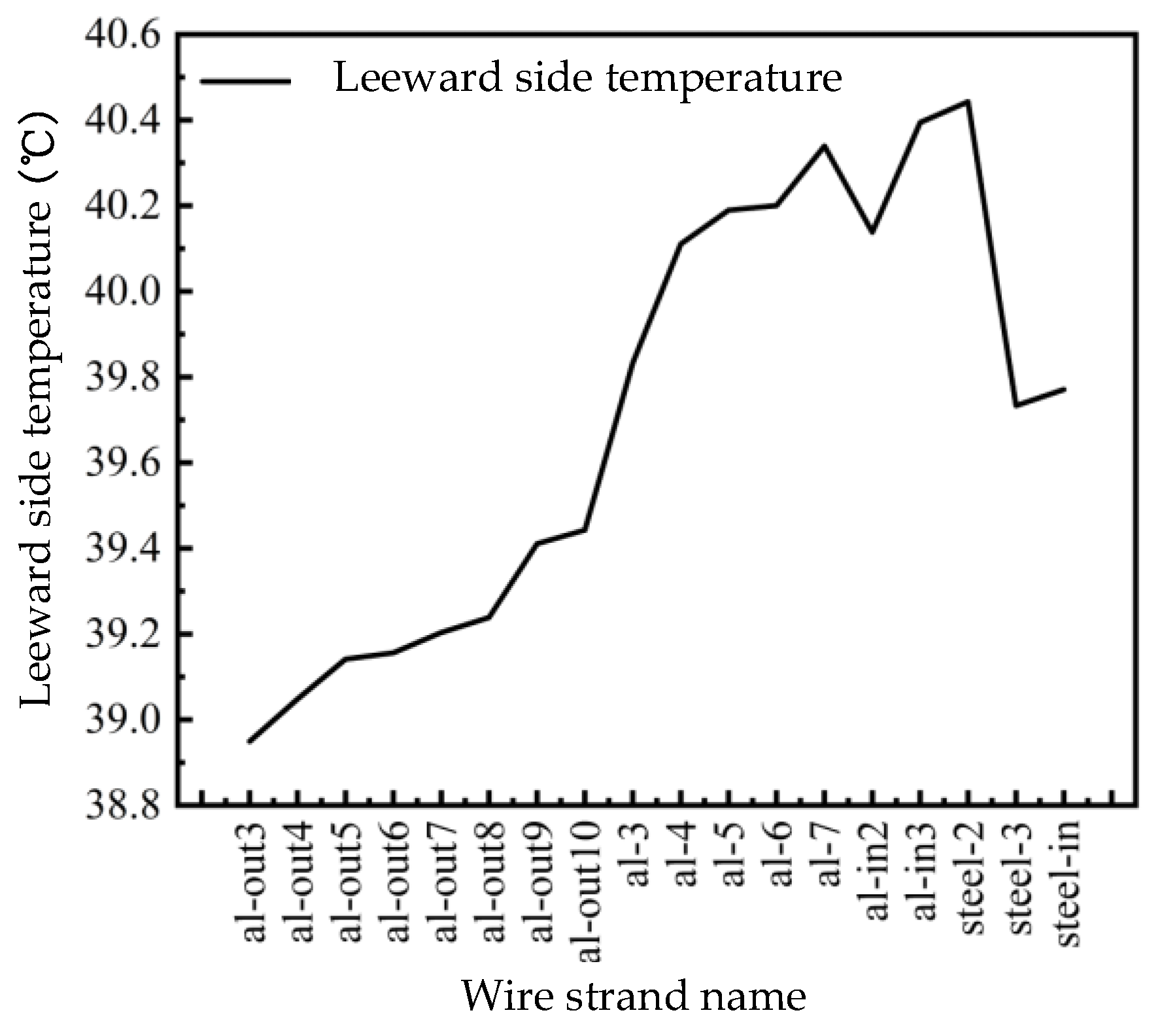
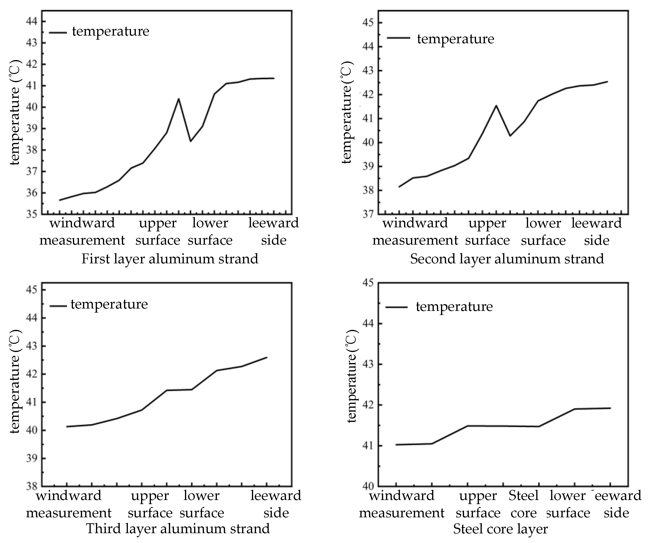
2.2.1. Temperature Distribution of Conductor Strands

The temperature difference in the line is mainly due to two factors: firstly, there is a skin effect in the current, which causes a temperature difference between the outer and inner layers of the conductor. The second is air flow, which has different convective heat transfer effects at different positions on the surface of the conductor, resulting in temperature differences at different positions on the surface [20].

In order to achieve the calculation of the two factors, we established a finite element model and analyzed the radial temperature distribution of the conductor under different current carrying capacities and environmental conditions. Taking LGJ-400/35 as an example, a three-dimensional physical model of a conductor was constructed. The conductor is composed of 7 steel cores with a radius of 1.25 mm and 48 aluminum strands with a radius of 1.61 mm, and the adjacent layers of strands are twisted in reverse, as shown in Figure 2.

Firstly, the fluid domain has a relatively large mesh size due to its large volume and not being the main part of the simulation. Secondly, there is the conductor part, which is the main part of grid division. The conductor strands are twisted, and the air gap between the conductors is narrow and sharp. Therefore, grid division needs to be refined and encrypted separately, with the smallest grid division size. The grid division diagram and detailed diagram are shown in Figure 3. In the diagrams, the two colored arrows represent the inlet and outlet of natural wind, respectively.

Due to the different materials and resistances of the inner and outer layers of the conductor, the heat flux generated by the steel core and aluminum strand varies. Therefore, when calculating the heat generation rate of conductor strands, the heat generation rate of the aluminum strands and steel cores is calculated separately based on the current flowing through the conductor and electromagnetic induction. In addition, due to the physical structural characteristics of the conductor itself, the outermost aluminum strand of the conductor is affected by solar radiation and wind speed. Therefore, the outermost aluminum strand of the conductor requires separate application of solar radiation heat. Finally, environmental parameters such as temperature, wind speed, and wind direction are set as boundary conditions for simulation operations based on on-site operational data. The simulation flow chart is shown in Figure 4.

According to the heat balance equation, the factors that affect the operating temperature of transmission conductors include surface morphology, physical parameters, environmental temperature, environmental wind speed, sunlight intensity, surface radiation coefficient, and conductor absorption coefficient. However, during the actual operation of conductors, the surface morphology, physical parameters, surface radiation coefficient, and surface absorption coefficient are all determined, and the temperature difference in the conductor strands mainly comes from the influence of environmental wind speed. Therefore, based on the established conductor model, this article analyzes the effects of different wind speeds on the radial temperature distribution characteristics of the conductor.

During the calculation, it was determined that the sunlight intensity was 1000 W/mm², the ambient temperature was 20 °C, and the conductor current carrying capacity was 400 A. The radial temperature distribution characteristics of the conductor were obtained when the wind speed was in steps of 0.5 m/s from 0 to 5 m/s. Figure 5 shows the temperature distribution when the wind speed was 2 m/s.

From Figure 5, it can be seen that the radial temperature distribution of the conductor is uneven, and the surface temperature on the windward side is significantly lower than that on the leeward side, with a maximum difference of 4.09 °C. Taking the top conductor of each layer as the reference point, the first layer strand is named al-out1, the second layer strand is named al-1, the third layer strand is named al-in1, and the steel core layer strand is named steel. For steel-1 and steel-in, we counted the conductors in a clockwise direction. Figure 6 shows the temperature values of each strand on the leeward side.

For the convenience of calculation and measurement, we divided the conductor into four parts: the windward area, leeward area, upper area, and lower area (as shown in Figure 7).

The division of regions is based on the Karman vortex street effect of airflow on the surface of the conductor. Figure 8 shows the temperature distribution of each layer of the conductor strand in different regions.

Each layer of the conductor strands exhibits the lowest temperature on the windward side. Owing to the gradual heat dissipation in the air gaps and swift metal-to-metal contact heat transfer, the temperature on the leeward side reaches its peak, while the temperatures on the upper and lower surfaces remain relatively uniform. Progressing from the first layer to the steel conductor layer, the windward-side temperature incrementally rises, with the highest temperatures on the upper and lower surfaces and the leeward side typically occurring in the second or third layer of the conductor. The temperature variation on the leeward side of each layer is minimal, influenced by the heat conduction and dissipation methods, which are contingent on the air domain’s dimensions. The first layer of conductor strands dissipates heat through metal-to-metal conduction and convective heat dissipation in the air. The subsequent layers dissipate heat through metal-to-metal transfer and air gap heat transfer. Notably, the windward side of the first layer experiences rapid convective heat dissipation due to wind speed, while other layers maintain lower temperatures due to metal-to-metal heat transfer. The upper and lower surfaces of the first layer, along with the leeward side, directly contact the air, facilitating faster heat dissipation. Owing to the smaller air gap, slower heat dissipation, and elevated temperatures in other layers, the highest temperature point often arises in the second or third layer. Ultimately, the leeward-side conductor’s temperature fluctuation is insignificant, attributable to the faster solid heat transfer rate compared to gas heat transfer rate.

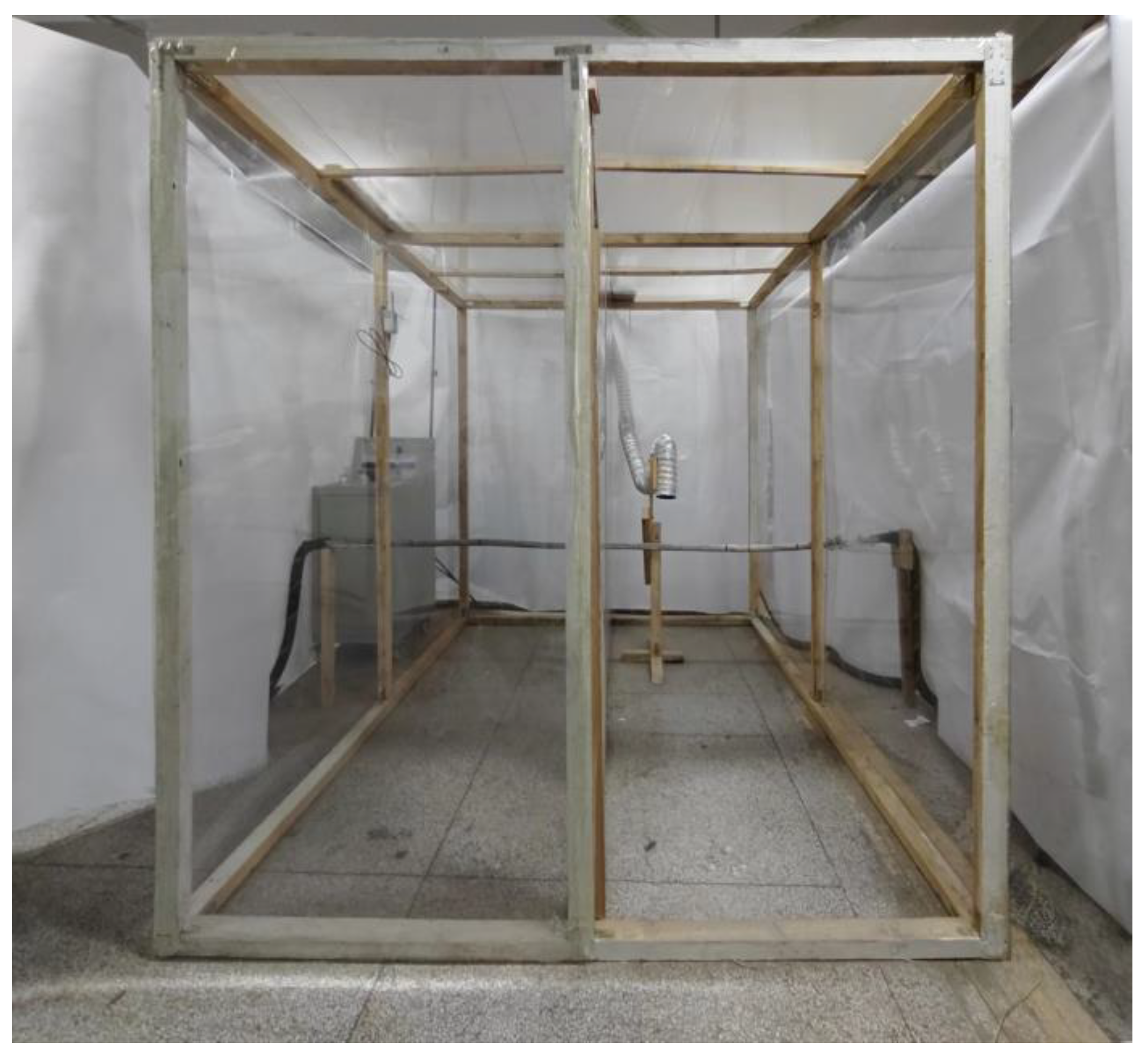
2.2.2. Experiment on Temperature Difference between Layers

To further validate the method’s effectiveness, we conducted experiments to examine the impact of wind on surface temperature, employing the same model of a steel-core aluminum-stranded conductor under conditions consistent with the simulation. Figure 9 shows the experimental platform. A current regulator was utilized to supply current to the conductor, an axial fan was employed to induce airflow, and an infrared thermal imager was used to monitor the conductor’s temperature. Prior to the experiment, the conductor’s surface was meticulously cleaned to prevent measurement errors stemming from variations in surface dirt and the infrared reflectance of the conductor body.

The measured temperatures on the upper surface, lower surface, windward side, and leeward side of the conductor are shown in

Table 1. Experimental data table of conductor surface temperatures.

Area	Windward Side	Upper Surface	Lower Surface	Leeward Side
Temp. (°C)	37.1	39.2	38.8	41.5

.

The middle temperature of each region in the table represents the temperature of the region. Although there are some differences between the experimental and finite element simulation results, it can be seen that the surface temperature distribution pattern is indeed consistent with the simulation.

2.2.3. Length Calculation Considering Temperature Distribution

Due to the different temperatures of each layer of the conductor, the radial thermal expansion of each strand is different, so the elongation of each strand is also different. Taking a strand of conductor as an example, we unfolded it to obtain the geometric relationship between the elongation of each strand of conductor and the total elongation of the conductor. The unfolding diagram of a strand of conductor is shown in Figure 10.

The elongation of a conductor is a function of the total elongation generated by stress and thermal expansion, which represents the calculation formula for the conductor:

$$\{\begin{array}{l}{\epsilon }_{ia}={\epsilon }_0{\sin }^2(a_{ia}+\Delta a_{ia})-\frac{\Delta R_{ia}}{R_{ia}}{\cos }^2(a_{ia}+\Delta a_{ia})\\ {\epsilon }_{is}={\epsilon }_0{\sin }^2(a_{is}+\Delta a_{is})-\frac{\Delta R_{is}}{R_{is}}{\cos }^2(a_{is}+\Delta a_{is})\end{array}$$

(4)

where ${\epsilon }_0$ is the total elongation of a conductor caused by stress and thermal expansion; $\Delta a_{ia}$ and $\Delta a_{is}$ are the angle increments generated by tension on the aluminum strand and steel core, respectively, but for any strand of conductor, the angle between each strand of the conductor and the cross-section $\Delta a_{ia}$ or $\Delta a_{is}$ is far greater than the angle increment caused by tension $\Delta a_{ia}$ or $\Delta a_{is}$. Therefore, the angle increment can be ignored; $R_{ia}$ and $R_{is}$ are the radii of the aluminum strands and steel cores, respectively; $\Delta R_{ia}$ and $\Delta R_{is}$ are the radius increments generated by the radial thermal expansion of the conductor for aluminum strands and steel cores, respectively.

The calculation formula for the thermal expansion of conductors is

$$\{\begin{array}{l}\Delta R_{ia}={\alpha }_{ia}{R}_{ia}(T_{ia}-T_a)(i=1,\cdots ,24)\\ \Delta R_{is}={\alpha }_{is}{R}_{is}(T_{is}-T_a)(i=1,\cdots ,7) \end{array}$$

(5)

By introducing the two formulas in Equation (5) into the two formulas in Equation (4), the relationship between the elongation generated by each aluminum strand and steel core and the total elongation of the conductor can be obtained separately. Finally, based on the equal axial internal and external forces of the conductor, the total elongation of the conductor caused by stress and thermal expansion can be obtained, ${\epsilon }_0$.

2.3. Correction Calculation Method for Sag

After considering the temperature difference in the conductor strands, the corrected total elongation change in the conductor can be obtained, and its calculation formula is

$${\epsilon }_T={\overline{\epsilon }}_0+{\epsilon }_c-{\epsilon }_{{\sigma }_0}$$

(6)

$${\epsilon }_{{\sigma }_0}=\frac{{\sigma }_0{A}_0}{E_{ia}{A}_{ia}+E_{js}{A}_{js}}$$

(7)

where ε_T is the change in total elongation in the conductor and ${\epsilon }_{{\sigma }_0}$ is the conductor elongation caused by σ₀.

The initial arc length of the conductor can be obtained based on the initial stress per unit area, and its calculation formula is

$$L_0=\sqrt{{\left(\frac{2{\sigma }_0}{\gamma }\sinh \frac{\gamma l}{2{\sigma }_0}\right)}^2+h^2}$$

(8)

After considering the radial temperature, the initial arc length of the conductor is corrected to obtain a more accurate arc length of the conductor. The calculation formula is

$$L=L_0(1+{\epsilon }_T)$$

(9)

Due to the unknown initial arc length, the initial stress per unit area is not accurate. Therefore, this article uses the modified conductor arc length to calculate the conductor sag, and the calculation formula is

$$f_M=\sqrt{(L-\frac{l}{\cos \varphi })\cdot \frac{3l}{8{\cos }^2\varphi }}$$

(10)

For operational conductors, the first step involves deriving catenary equation based on the geometric characteristics of single-span overhead lines. Next, the article addresses the radial temperature distribution pattern of the conductor, acknowledging that the force on each conductor is not uniform. Considering the uneven radial temperature distribution of the conductor, the article also takes into account the influence of radial thermal expansion. Finally, Using Formulas (4) and (5) calculate the total axial internal force of the conductor. The total elongation of the conductor, resulting from the balance of internal and external forces, is then deter-mined. Lastly, the typical creep value and Formula (7) are substituted into Formula (6) to calculate the total elongation change of in the conductor. This information, along with Formulas (6), (8) and (9), is incorporated into (10) to obtain the corrected sag.

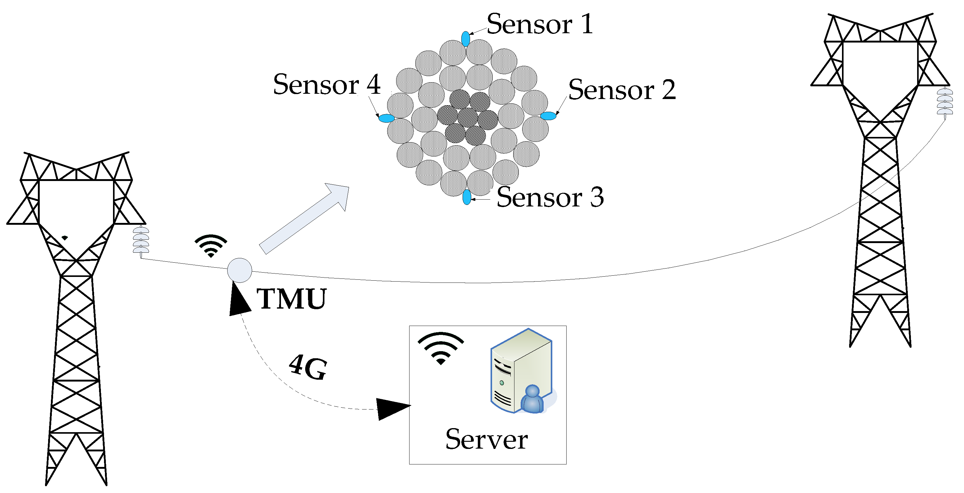
3. Sag Monitoring Method

According to the previous analysis, the method of monitoring conductor sag based on temperature collection must consider the temperature differences at multiple points. Therefore, we have designed a multi-point temperature acquisition sag monitoring system, with the system architecture shown in Figure 11. The system mainly includes two parts: temperature measurement unit and server.

A temperature measurement unit (TMU) is installed on the conductor, incorporating four sensors to measure the temperature of the upper, lower, windward, and leeward areas of the conductor independently. Throughout the measurement process, the sag value is calculated based on the temperature values at each measuring point, and the resulting data are transmitted to the service server through 4 G.

To extend operational hours, each component of the sensor is selected for low power consumption. Given the necessity to execute the calculation formulas from Section 2 on the CPU, the STM32L052 microprocessor is chosen for its simplicity in computation. Featuring a 32-bit RISC architecture, the STM32L052 microprocessor has a maximum operating speed of 32 MHz and a minimum current of 0.8 μA in Stop mode, coupled with 8 kB of RAM to meet operational requirements. Despite the STM32L052 microprocessor having a 12-bit integrated ADC, the AD7682 is selected to attain the minimum resolution required.

For sensor power supply, the principle of electromagnetic induction is employed to charge lithium batteries. The power controller encompasses charge–discharge control and protection circuits. In instances of high load currents, such as during a short-circuit, the power controller can execute charge–discharge control. Additionally, multiple load switches are incorporated into the controller and management module to achieve energy efficiency.

4. Field Test and Discussion

The monitoring device and sag calculation method were tested in Qinghai, China, with sensors installed on conductors. The span was 670 m, with a height difference angle of 2.56°, as shown in Figure 12.

Utilizing TMU measurements with theodolite measurements as a reference, we compared the error magnitude between the single-point temperature measurement method and the four-point temperature measurement method for sag calculation. We derived the relative error of sag through multiple measurements while concurrently recording the wind speed. The data presented in

Table 2. Measured data.

Time	Theodolite Measurement (m)	Wind Speed (m/s)	4-Point Temp. Meas.		1-Point Temp. Meas.
			Sag (m)	Relative Error	Sag (m)	Relative Error
12:50	32.54	2.1	32.15	1.20%	31.11	4.39%
13:50	31.66	4.8	31.20	1.45%	29.17	7.86%
14:50	33.99	0.5	33.36	1.85%	33.29	2.06%
15:50	32.01	2.7	31.58	1.34%	30.63	4.31%
16:50	31.51	4.0	30.98	1.68%	30.04	4.67%

pertain to measurements taken on 7 September 2023. To mitigate the impact of data fluctuations or noise on potential single sampling value drifts during the collection process, the current sampling value was determined as the average of 10 actual measurements.

From Table 2, it can be seen that at a wind speed of 0.5 m/s, the sag calculated through single-point temperature measurement and four-point temperature measurement was very close to the results measured using a theodolite. At this point, the relative error of single-point temperature measurement was 2.06%, while for four-point temperature measurement, it was 1.85%. This is because the wind speed was too slow, so the convective heat dissipation had almost no effect on the conductor temperature. When the wind speed reached 4.1 m/s, the relative error of single-point temperature measurement was significantly greater than that of four-point temperature measurement, as the convective heat dissipation at this time had a significant impact on the conductor temperature.

5. Conclusions

In this paper, a sag calculation model incorporating the radial temperature gradient and thermal expansion of the conductor is introduced. The traditional conductor sag model was enhanced, and its accuracy was validated through on-site measurement data. The impact of radial thermal expansion on conductor sag was analyzed, leading to the following conclusions:

The convective heat dissipation induced by wind significantly influences the temperature distribution of each strand of the conductor. For the steel-core, aluminum-stranded conductor with the model LGJ-400/35, the surface temperature of the windward-side strand was over 4 °C lower than that of the leeward-side strand. The temperature difference among conductor strands was notable. Taking this temperature difference into account, the calculation formula for the conductor length was revised, leading to an adjustment in the sag calculation method.

Based on the analysis of measured data from a ±400 kV transmission line in Qinghai, it is evident that at low wind speeds, the monitoring sag error using the single-point temperature measurement method is 2.06%, while the error with the four-point temperature measurement method is 1.85%, indicating a close correspondence. However, with increasing wind speed, a substantial difference in error values emerges between the two measurement methods. The error for the single-point temperature measurement method rises significantly to 7.86%, whereas the error for the four-point temperature measurement method consistently remains below 2%. Therefore, employing the four-point temperature measurement method for sag monitoring can significantly enhance measurement accuracy and ensure the safety of transmission lines.

Furthermore, considering surface damage and other phenomena along the wire’s direction, temperatures at different positions may exhibit variations. As a next step, we plan to investigate the influence of axial temperature differences on temperature to enhance the accuracy of sag calculations.

References

1. IEEE Std 1863–2019; IEEE Guide for Overhead AC Transmission Line Design. IEEE: New York, NY, USA, 11 May 2020; pp. 1–109.
2. Oluwajobi, F.I. Effect of sag on transmission line. J. Emerg. Trends Eng. Appl. Sci. 2012, 4, 627–630. [Google Scholar]
3. Yan, D.; Liao, Y. Online estimation of power transmission line parameters, temperature and sag. In Proceedings of the North American Power Symposium, Boston, MA, USA, 4–6 August 2011. [Google Scholar]
4. Polevoy, A. Impact of Data Errors on Sag Calculation Accuracy for Overhead Transmission Line. IEEE Trans. Power Deliv. 2014, 5, 2040–2045. [Google Scholar] [CrossRef]
5. Barrett, J.S.; Dutta, S.; Nigol, O. A New Computer Model of ACSR Conductors. IEEE Trans. Power Appar. Syst. 1983, 3, 614–662. [Google Scholar] [CrossRef]
6. Alawar, A.; Bosze, E.J.; Nutt, S.R. A hybrid numerical method to calculate the sag of composite conductors. Electr. Power Syst. Res. 2006, 5, 389–394. [Google Scholar] [CrossRef]
7. Bedialauneta, M.T.; Fernandez, E.; Albizu, I. Sag-tension evaluation of high-temperature gap-type conductor in operation. IET Gener. Transm. Distrib. 2022, 1, 19–26. [Google Scholar] [CrossRef]
8. Agüero-Rubio, J.; López-Martínez, J.; Gómez-Galán, M.; Callejón-Ferre, Á.-J. A Didactic Procedure to Solve the Equation of Steady-Static Response in Suspended Cables. Mathematics 2020, 8, 1468. [Google Scholar] [CrossRef]
9. Kamboj, S.; Dahiya, R. Designing and implementation of overhead conductor altitude measurement system using GPS for sag monitoring. In Proceedings of Intelligent Computing Techniques for Smart Energy Systems; Springer: Singapore, 2019. [Google Scholar]
10. Mensah-Bonsu, C.; Krekeler, U.F.; Heydt, G.T.; Hoverson, Y.; Schilleci, J. Application of the Global Positioning System to the measurement of overhead power transmission conductor sag. IEEE Trans. Power Deliv. 2002, 1, 273–278. [Google Scholar] [CrossRef]
11. Safdarinezhad, A.; Abdollahifard, M.J.; Ganjali, A. A photogrammetric solution for measurement of power lines sag via integration of image and accelerometer data of a smartphone. Measurement 2022, 199, 111493. [Google Scholar] [CrossRef]
12. Song, J.; Qian, J.; Liu, Z.; Jiao, Y.; Zhou, J.; Li, Y.; Chen, Y.; Guo, J.; Wang, Z. Research on Arc Sag Measurement Methods for Transmission Lines Based on Deep Learning and Photogrammetry Technology. Remote Sens. 2023, 15, 2533. [Google Scholar] [CrossRef]
13. Hlalele, T.S.; Du, S. Real time monitoring of high voltage transmission line conductor sag: The state-of-the-art. Int. J. Eng. Adv. Technol. 2013, 1, 297–302. [Google Scholar]
14. Rodriguez, J.; Franck, C.M. Dynamic Line Rating of overhead transmission lines under natural convective cooling. In Proceedings of the IEEE Eindhoven PowerTech, Eindhoven, The Netherlands, 2 July 2015. [Google Scholar]
15. Song, N.; Yangchun, C.; Yuan, D. A new sag calculation method based on the temperature of overhead transmission line. J. North China Electr. Power Univ. 2013, 6, 27–32. [Google Scholar]
16. Guo, D.; Wang, P. Investigation of Sag Behaviourfor Aluminium Conductor Steel Reinforced Considering Tensile Stress Distribution. R. Soc. Open Sci. 2021, 8, 2–16. [Google Scholar] [CrossRef] [PubMed]
17. Liu, Y.; Chen, Z.; Gu, Q. Numerical Algorithms for Calculating Temperature, Layered Stress, and Critical Current of Overhead Conductors. Math. Probl. Eng. 2020, 2020, 6019493. [Google Scholar] [CrossRef]
18. Wang, K.; Sun, X.; Sheng, G. Error comparison among three on-line monitoring methods of conductor sag of overhead transmission line. High Volt. Appar. 2014, 4, 27–34. [Google Scholar]
19. Ramachandran, P.; Vittal, V.; Heydt, G.T. Mechanical State Estimation for Overhead Transmission Lines with Level Spans. IEEE Trans. Power Syst. 2008, 3, 908–915. [Google Scholar] [CrossRef]
20. Dong, X.; Wang, C.; Liang, J.; Han, X.; Zhang, F.; Sun, H. Calculation of Power Transfer Limit Considering Electro-Thermal Coupling of Overhead Transmission Line. IEEE Trans. Power Syst. 2014, 4, 1503–1511. [Google Scholar] [CrossRef]
Figure 1. Schematic diagram of sag.
Energies 17 00305 g001
Figure 2. Conductor model diagram: (a) cross-section view; (b) side view.
Energies 17 00305 g002
Figure 3. Schematic diagram of the three-dimensional model grid of LGJ400/35.
Energies 17 00305 g003
Figure 4. The process of finite element calculation of temperature.
Energies 17 00305 g004
Figure 5. Conductor temperature distribution diagram.
Energies 17 00305 g005
Figure 6. Temperature distribution of conductor strands.
Energies 17 00305 g006
Figure 7. Regional division.
Energies 17 00305 g007
Figure 8. Temperature distribution of conductor strands in each layer.
Energies 17 00305 g008
Figure 9. Temperature experiment.
Energies 17 00305 g009
Figure 10. Unfolded view of one strand of conductor.
Energies 17 00305 g010
Figure 11. System architecture.
Energies 17 00305 g011
Figure 12. Field test.
Energies 17 00305 g012