1. Introduction
With recent advances in computer processing power and the development of artificial intelligence, the application of artificial intelligence has expanded into many fields. Turbine aerodynamic optimization, traditionally dependent on expert knowledge, has seen a paradigm shift with the adoption of advanced techniques. These include artificial neural networks (ANNs), particle swarm optimization (PSO), genetic algorithms (GAs), and statistical methods like response surface methodology (RSM).
In the early stages, the neural network (NN) model began to be widely used in the 1980s based on its advantage of being applicable to functions that cannot be represented by polynomials. Initially, it was primarily used for diagnostics and maintenance purposes. Later on, its effectiveness in the control of non-normal aerodynamic conditions was also demonstrated. According to Greenman’s research [
1], NNs were used for the optimization of airfoils with high-lift performance, reducing the resources required for optimization by 44% compared to traditional gradient-based optimization methods. Rai and Madavan [
2] highlighted the effectiveness of NNs in the inverse design of turbomachinery, particularly for estimation and prediction. Additionally, it was reported that combining response surface methodology (RSM) with NNs had advantages in addressing high-dimensional problems. After the proposal of backpropagation neural networks (BPNN), they were found to be more effective in predicting parameters like drag and lift coefficients [
3]. However, BPNNs were sometimes slow and less efficient than other NNs for specific problems due to error propagation from one layer to the next. To address these drawbacks, radial basis neural networks (RBNN) were introduced. RBNN models are relatively computationally efficient as they use linear regression and are known for their high accuracy and broad applicability when non-linear results are required. In comparison to BPNN, RBNNs are more efficient when a large amount of training data is available [
4,
5].
Further into the development of machine-learning-based optimization, research has reported the use of combined optimization techniques or multi-objective function optimization. Samad et al. [
6] conducted a study on compressor optimization with multiple objective functions using various surrogate models (PBA, RBNN, RSA, KRG). They reported that combining surrogate models can enhance the robustness of optimization. Typically, the statistical approach of the PRESS-based averaging (PBA) method, which evaluates the predictive power of regression, is used for combining surrogate models. Specifically, through PBA, the combination of surrogate models is achieved by assigning higher weights to models with higher accuracy. A similar approach has also been reported for evaluating cavitation models through global sensitivity analysis [
7]. Pierret, S., and Van [
8] derived optimal shapes through simulated annealing (SA) and surrogate model development, then validated the performance using computational fluid dynamics (CFD). They reported the ability to satisfy both mechanical and aerodynamic conditions by developing objective functions, demonstrating the feasibility of fully automated optimization. Shyy, W., et al. [
9], on the other hand, reported optimization of rocket propulsion components such as injectors, supersonic turbines, and diffusers using response surface methodology (RSM) and ANNs. According to their findings, global optimization can handle multiple design points and trade-offs, provide multi-criterion optimization, and filter noise originating from numerical analysis and experiments. Importantly, they highlighted the effectiveness of both response surfaces and neural networks when results from numerical computations, experiments, and theoretical calculations need to be combined.
In recent years, gas turbine research has seen an inclination towards advanced methodologies. Liu, Z., and Karimi [
10] developed two surrogate models using ANN and high-dimensional model representation (HDMR) with actual operational data. Integrated into a simulation model, these surrogates performed well at partial and full loads. Du, Q., et al. [
11] employed a dual deep learning model for axial turbine performance prediction, achieving relative errors of less than 0.85% compared to CFD results. Akolekar, H. D., et al. [
12] addressed laminar kinetic energy model limitations using a CFD-driven multi-objective (MO) model, outperforming the single-objective (SO) model. In ORC-focused studies, challenging conditions led to innovative approaches. Xu, G., et al. [
13] optimized a radial-axial two-stage turbine using GA for supercritical conditions. Witanowski, Ł. et al. [
14] optimized an axial turbine with R7100 using the Nelder–Mead method. Variable impact comparison revealed a 30% performance decrease with a 60% computation time reduction. Jankowski, M., et al. [
15] used NSGA (non-dominated sorting genetic algorithm)-II and TOPSIS (technique for order preference by similarity to ideal solution) for R1234yf turbine optimization, with a 7:3 weighting between electricity cost and turbine size as objective functions. Wang, Y., et al. [
16] compared SA, improved SA, and GA for a radial inflow turbine, reporting a 5% isentropic efficiency increase and 59.6% time reduction with improved SA. Similar endeavors were noted in wind and tidal turbines. Studies combined ANN and wake models for wind turbine power modeling and determined optimal yaw angles [
17]. MO models with genetic optimization were used for tidal turbine optimization, and the results were validated through model tests and sea trials [
18].
Drawing upon previous research, various artificial intelligence models have been applied for the shape optimization of gas turbines, ORC turbines, and wind and tidal turbines. Additionally, studies [
19,
20,
21] have explored the thermodynamic cycles and turbines for replacing HFC (hydrofluorocarbon) refrigerants, such as R245fa, with HFO (hydrofluoroolefin) refrigerants, exemplified by R1233zd. However, to date, there appears to be a lack of reported research applying RBNN models for the optimization of a two-stage radial turbine utilizing R1233zd(e) refrigerant for medium- to low-temperature heat sources. In this study, we conducted research on the optimization of a turbine in an ORC system utilizing waste heat from ship engines. The turbine in this system operates with R1233zd(e) as the working fluid and is configured as a back-to-back two-stage radial turbine with a target power output of 100 kW. Operating conditions are 25,500 rpm rotational speed, 155 °C inlet temperature, 2094 kPa inlet pressure, and 250.5 kPa outlet pressure (expansion ratio of 8.4). To ensure optimal performance, artificial neural networks (RBNN), design of experiments (DOE), and Latin hypercube sampling (LHS) were applied together.
2. Optimization of ORC Turbine with RBNN
2.1. ORC Turbine Design
In this study, a 100 kW-rated ORC turbine was required to utilize waste heat from ships. In consideration of the environmental impact, R1233zd(e) was chosen as the working fluid for the waste heat recovery system, aiming to achieve high efficiency. The refrigerant R1233zd(e) belongs to ASHRAE’s safest category, group A1. It possesses a low global warming potential (GWP) and serves as a viable substitute for the widely used R245fa. Its application as an alternative refrigerant showcases comparable efficiency in organic Rankine cycle power generation systems. To ensure high efficiency in a system with an expansion ratio of 9 and to counteract axial forces, a two-stage radial turbine with a back-to-back configuration was selected (see
Figure 1 and
Table 1).
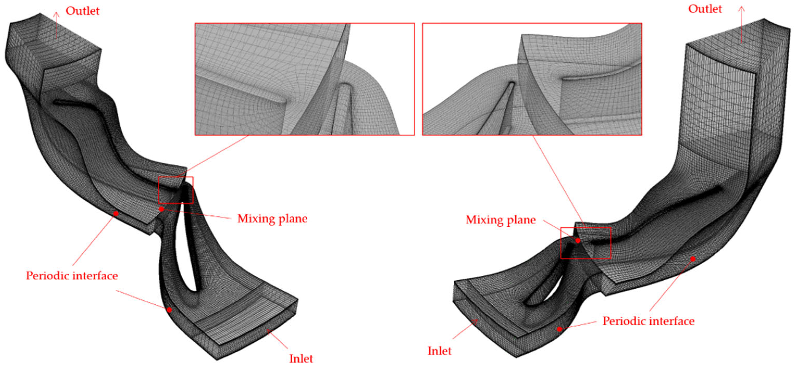
To operate two turbines coaxially in a back-to-back structure, the rotation directions of the two turbines are opposite. To improve performance at the design point and compare results between the optimization design and the design point, numerical analysis was performed. To perform optimization separately for each turbine, the first and second stages of the turbine were analyzed separately. The turbulence model used in the study is the shear stress transport (SST) model. The computational domain consists of four regions: inlet, nozzle, rotor, and outlet. Periodic boundary conditions were applied for the boundary conditions in the direction of rotation. The region where the nozzle and rotor are connected was treated with a mixing-plane (constant total pressure) boundary condition. Inlet conditions were given as pressure conditions, and outlet conditions were given as pressure conditions as well. The analysis for the entire system of the first and second stages was performed separately because grid generation and analysis consumed a significant amount of time. Both turbines were designed with shrouded covers to minimize tip clearance loss. Therefore, in the analysis conditions, tip clearance was set to 0.
The properties of the working fluid R1233zd(e) were modeled as a single-phase vapor model using the Peng–Robinson state equation. The grid resolution was determined using grid convergence index (GCI) calculations, with each of the first and second stages of the turbine having approximately 500,000 grid cells. The mesh was generated using the ATM (adjoint-turbulence model) topology in the Turbogrid program to appropriately account for the flow boundary layer and ensure the robustness of the simulation. Key boundary conditions, along with the generated mesh and zoomed-in illustrations at the interfaces of the first and second stages, can be observed in
Figure 2.
Based on the numerical analysis results before optimization, the first stage achieved a total-to-total isentropic efficiency (Equation (1)) of 91.1%, and the second stage achieved efficiency of 86.4% at the design point. Design points (temperature, pressure, and rotational speed) are as shown in
Table 1. In this study, boundary conditions for all analysis cases were defined using design points instead of globally varying temperature and pressure conditions. The rationale behind this choice is to validate the effectiveness of the turbine optimization methodology employing the RBNN model.
2.2. Grid Dependency and Discretization Error
Residual comparison and the calculation of GCI [
22] were conducted to assess grid dependency and discretization errors. Our findings revealed that total-to-total isentropic efficiency, pressure ratio, and residuals converged after 3500 iterations. As shown in
Figure 3, each efficiency reached convergence levels of 90.4% (Mesh 1), 90.5% (Mesh 2), and 91.0% (Mesh 3), respectively. Similarly, it can be observed that the pressure ratio also converges to 2.9 for all meshes after 3000 iterations. Here, the pressure ratio is defined as the ratio of the inlet pressure to the outlet pressure.
Table 2 presents the average root mean square (RMS) residual at the end of the iterations. The residuals exhibited convergence with oscillatory behavior. The average was computed over the oscillation period, which spanned approximately 20 iterations, to minimize its impact. This oscillatory behavior appears to arise as a transient phenomenon due to less-than-optimal turbine design, resulting in the generation of eddy currents within the rotor. Additionally, our results indicate that increasing the number of grid points leads to a slight reduction in residual values.
The GCI method quantitatively presents discretization errors through uncertainty ratios and values obtained via extrapolation. The estimation of discretization errors proceeds as follows: three numerical analysis models are created with different grid resolutions, numerical analyses are conducted, GCI’s main parameters are calculated using the simulated results, and extrapolation values and uncertainties are computed [
23]. As the initial step, three models with varying grid resolutions were generated (refer to
Table 3). Depending on the grid refinement ratio (r), the relative error may be either overestimated or underestimated; hence, a threshold of 1.3 or higher is required, based on experimental recommendations. In this study, the grid refinement ratio is approximately 1.35, as indicated in
Table 4. Note that Φ represents the parameter value for each model (such as flow rate, power, total-to-total isentropic efficiency, and total enthalpy), while ε denotes the difference between these parameters, and ‘s’ is the sign function of the ratio of ε
32 to ε
21, with a negative value indicating oscillatory convergence. As depicted in
Table 4, both enthalpy and power exhibit oscillatory convergence. As previously mentioned, this behavior appears to stem from vortices generated within the rotor due to its non-optimized shape.
Subsequently, the following values are calculated sequentially: the extrapolation value (Φext), relative error (ea), extrapolation value and relative error (eext), and GCI value. In the case of power estimation, when employing Mesh 1 and 2, the relative error was 0.95%, resulting in a GCI of 5.2%. When using Mesh 2 and 3 for estimation, the relative error reduced to 0.78%, yielding a GCI of 4.36%. Here, GCI represents the difference from the asymptote in scenarios where there is no discretization error. With Mesh 2 and 3, the mass flow rate, total-to-total isentropic efficiency during isentropic expansion, and GCI of total enthalpy at the outlet were sufficiently small, measuring at 0.75%, 0.01%, and 0.02%, respectively.
2.3. Turbine Design Parameter Change
The ORC system in this study places a significant emphasis on improving turbine efficiency, primarily due to its utilization of waste heat from maritime vessels. More specifically, this focus is driven by the need to accumulate economic benefits over the long-term operation of ships and to expedite the payback period, as well as to adhere to the International Maritime Organization’s (IMO) energy efficiency index regulations. To improve turbine efficiency, optimizing the turbine’s shape is necessary. There are various methods to adjust turbine shapes, so it is essential to choose appropriate variables that can be adjusted with minimal changes in the design process. The minimization of rotor shape modifications is motivated by the aim of reducing the extent of reworking components such as the housing, diffuser, and seals. This approach is driven by the desire to streamline the manufacturing process, thereby minimizing the need for extensive re-fabrication of components. The method proposed by Cho et al. [
24] was applied, which uses Bezier curves to represent the turbine’s shape. Using this approach, it becomes possible to alter the turbine’s shape with a small number of control points on the Bezier curves, and these control points can be selected as design variables. Consequently, it becomes feasible to change and represent the complex shape of the rotor with a limited number of control points.
Optimization was carried out by varying the meridional shape and the blade angles on both the hub and shroud surfaces of the rotor while keeping the number of variables to a minimum. To achieve this, seven Bezier control points were used for each rotor (two for rotor surfaces and five for rotor angles), in order to minimize the total number of variables.
Table 5 and
Table 6 show the Bezier control points and constraint values at the design point for the first- and second-stage rotors. Among the five Bezier control points, only the third control point was selected as a design variable for meridional shape. The blue line corresponds to a case where the design variable values are adjusted to increase, while the red line corresponds to a case where the values are adjusted to decrease.
The selected design variable control points in the rotor shape can be moved in the Z-direction (axial) and R-direction (radial), but in this study, only the R-direction (Φ1, Φ2, Ψ1, Ψ2) was adjusted.
Figure 4 illustrate the design values and the movement of Bezier control points from the initial point for the hub and shroud on the first rotor.
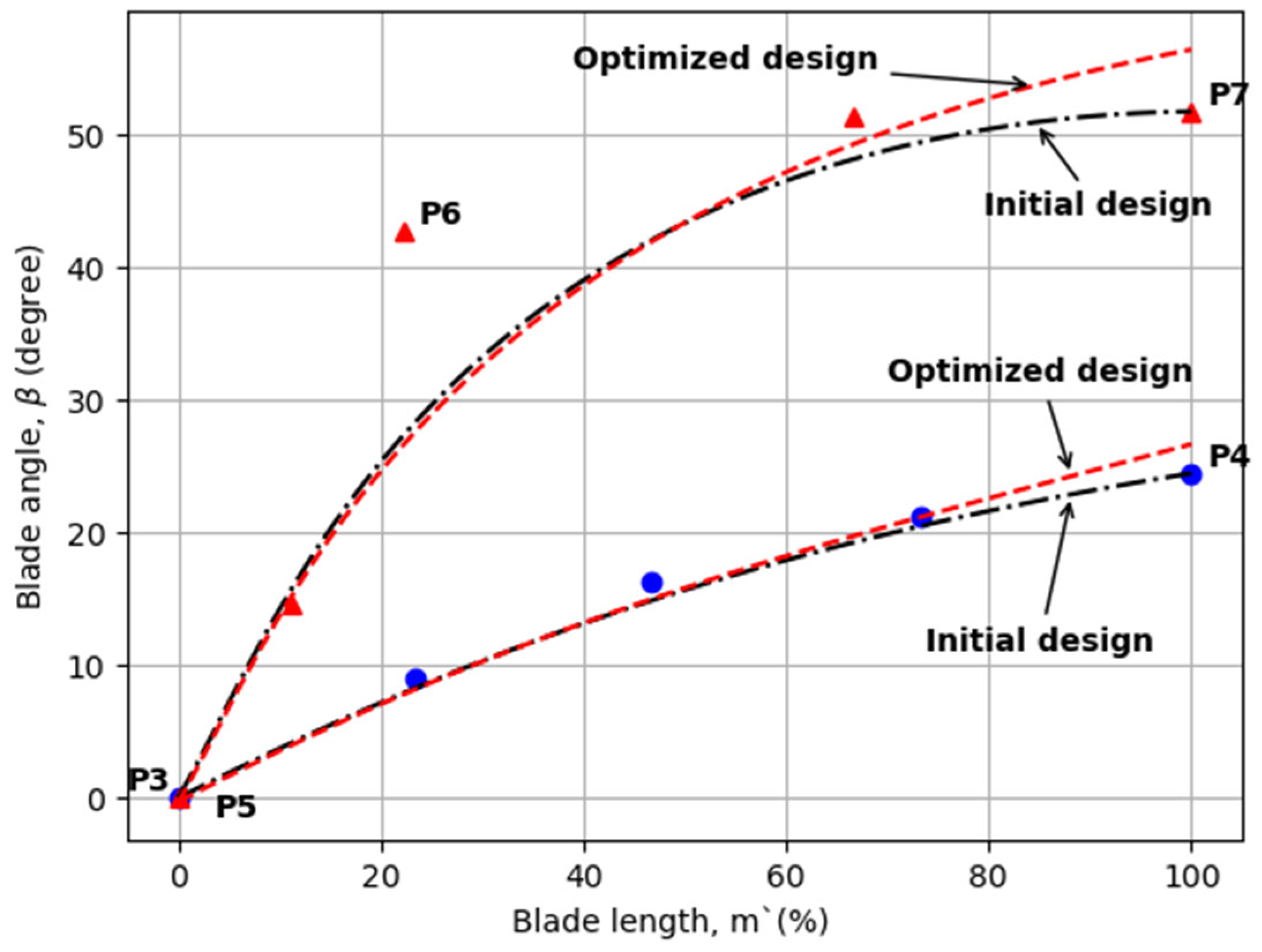
Among the five Bezier control points that determine the rotor angles, three points were selected as design variables for the shroud portion, while two were selected for the hub portion. The representation of the 3D blade angles was done using the blade angle (β) and the curved normalized length of the blade (m). The adjustment of the blade angle was chosen as design variables at the entrance, middle, and exit points for the shroud (first rotor—Φ5, Φ6, Φ7; second rotor—Ψ5, Ψ6, Ψ7). For the hub, the adjustment points at the entrance and exit were chosen as design variables (first rotor—Φ3, Φ4; second rotor—Ψ3, Ψ4). Due to the initial design where the blade angle for the second stage turbine is 0°, Ψ3 and Ψ5 remained unchanged at 0°, unlike Φ3 and Φ5 of the first stage, which were adjusted by a certain percentage (±10%) to account for angle changes. Consequently, a total of seven design variables (P1 to P7) were selected for each stage of the turbine rotor. The rotor shape was modified under minimal constraint conditions, and the values of the design variables and constraints can be found in
Table 5,
Table 6,
Table 7 and
Table 8. Additionally, the changes in the meridional blade shape for the first rotor and the angle changes can be observed in
Figure 4 and
Figure 5, respectively. The blue line corresponds to a case where the design variable values are adjusted to in-crease, while the red line corresponds to a case where the values are adjusted to decrease. The blade thickness was set to distribute the same thickness as given at the design point to maintain structural stability.
2.4. Design Optimization Method
In turbine rotor optimization, the objective function, such as total-to-total isentropic efficiency or power output, does not change linearly with design point variations. Therefore, global methods need to be employed for optimization. To expedite the optimization process while using global methods, DOE, the machine learning technique known as RBNN, and the LHS technique were used.
To gather the data needed for training the machine learning model to be applied in turbine rotor optimization, DOE was employed. Fractional factorial design provided by the Minitab program was utilized to fine-tune the seven design variables for each stage of the turbine, reducing the number of distinct shape conditions from the full factorial design’s 128 cases to 64. These 64 shapes were generated while adhering to the constraints specified in
Table 5,
Table 6,
Table 7 and
Table 8. Numerical analysis was performed on these 64 shapes obtained through DOE, and the objective function, which is total-to-total isentropic efficiency, was calculated. Using the efficiency (η
tt,s) values obtained through numerical analysis, input data for the machine learning model (RBNN) were created, and a trained model was implemented.
In this study, a radial basis neural network (RBNN), which is a type of shallow neural network, was employed to construct a surrogate model. RBNN is a recently developed multilayer neural network based on linear regression, known for its simplicity and fast computation. It consists of input, hidden, and output layers, as well as radial basis functions and linear outputs, as shown in
Figure 6. RBNN is chosen because it allows for nonlinear mapping, has a wide range of applications, and is suitable for interpolation and extrapolation. However, it may have increased computational costs when dealing with a large amount of data, and explaining the internal structure can be challenging in the case of multidimensional regression. RBNN was implemented using the newrb function, an embedded function in MATLAB (R2023a) program. Gaussian functions were used as the basis functions, and the output layer of RBNN is represented as Equations (2) and (3), where w represents the weight vector, p represents the input values, and b represents the bias values.
In the MATLAB program, to improve the accuracy of the RBNN model, it is important to choose appropriate error values and spread constants. The error and the number of iterations in RBNN are highly sensitive to the spread constant. In this study, RBNN models were implemented for the first-stage (spread constant = 10, error = 0.1) and the second-stage turbine (spread constant = 100, error = 0.1). The choice of these spread constant values (SC) was made by varying them from 0.1 to 1000 and selecting the SC values that resulted in the lowest error and iteration values.
After generating a surrogate model using the RBNN approach, this study involves the implementation of separate independent learning models for each stage. Subsequently, the Latin hypercube sampling technique is employed to obtain a substantial number of samples for each design variable, specifically 48,000 for each design variable. These cases are then applied to the trained RBNN models to identify the turbine shape that achieves the highest efficiency. Once the turbine shape with the highest efficiency is found within the design space, the optimization process concludes. If such an optimal turbine shape is not found, the number of design points generated by LHS is increased, and the process is repeated. This entire process is illustrated in a flow chart in
Figure 7.
3. Results and Discussion
Given the importance of efficiency in ORC turbines using waste heat from ships, the objective function for the RBNN model was set as total-to-total isentropic efficiency of the turbine. For both the first- and second-stage turbines, a total of 64 turbine efficiency values were obtained through DOE. These efficiency values were used to create surrogate models, and LHS technique was applied to find the design conditions that achieve the highest efficiency. Using the artificial intelligence model obtained through RBNN, it is possible to find the conditions that yield the highest efficiency by varying the design values within the constraints of the design variable conditions. The optimal design conditions for the first- and second-stage turbines obtained through the RBNN model are presented in
Table 9 and
Table 10. These results are also compared to the initial design in
Figure 8,
Figure 9,
Figure 10 and
Figure 11.
During the process of training the model using the RBNN method, both the design variable values and the objective function values should be normalized. Failure to normalize them could result in an inability to properly represent the influence of changes, especially for design variables with relatively small absolute values. In the MATLAB program, when training the RBNN model, the spread constant is adjusted to find the optimal value. The spread constant determines the range of influence of each neuron within each layer. By adjusting the spread constant and observing the optimal results, the appropriate value for this constant is determined for the model. In this study, a spread constant of 10 was applied to the first-stage turbine, and a spread constant of 100 was applied to the second-stage turbine. After five iterations, following the flow chart, improved efficiencies (η
RBNN) obtained were 92.78% for the first stage and 87.9% for the second stage. These results were more than 1.4% higher than the efficiencies of the initial design (
Table 1). However, since these results were obtained through the surrogate model, validation is necessary. To validate the obtained design variables through RBNN and LHS and confirm that they indeed yield high efficiency, numerical analyses were performed for each individual model using five cases. The same CFD methodology used for RBNN model training was applied. Total-to-total isentropic efficiencies (η
CFD) obtained through numerical analysis were 92.48% for the first stage and 87.62% for the second stage. In both sets of results, the efficiencies obtained through numerical analysis exceeded those from the initial design by 1.3% and 1.2%, respectively.
Figure 8 and
Figure 9 illustrate the results of the optimization for the first-stage turbine (highlighted in red). In terms of turbine geometry, the R value on the shroud side decreases, while the turbine blade angle at the hub side remains nearly unchanged. On the shroud side, which is denoted by the lower line in the illustration (
Figure 9), the blade angle exhibits a notable decrease, especially at the trailing edge.
Figure 10 and
Figure 11 compare the optimized geometry (highlighted in red) of the second-stage turbine with the initial design. In contrast to the first stage, the R value on the shroud side increased during the optimization. The blade angle, both at the hub and shroud, increased in the vicinity of the trailing edge as part of the optimization process.
The results presented in
Figure 12 and
Figure 13 demonstrate the validation of the optimization results using CFD. In
Figure 12, which represents the first-stage turbine, and
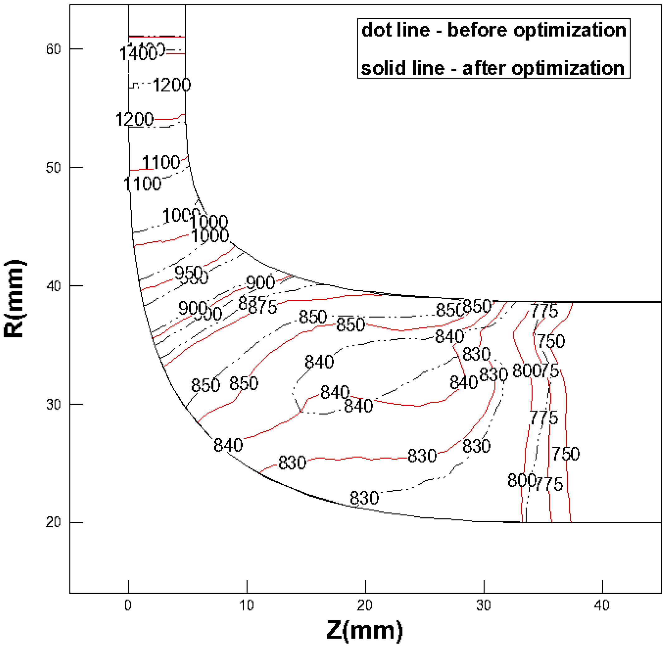
Figure 13, representing the second-stage turbine, the total pressure distribution is compared before and after optimization. In both turbines, it can be observed that the optimized turbines experience a delay in pressure drop. This indicates a reduction in the force losses due to expansion in the region where the flow expands, leading to an increase in turbine efficiency. In particular, for the first-stage turbine in
Figure 12, the pre-optimization results show inadequate pressure expansion, leading to a reverse flow phenomenon (840 kPa) in the middle. This reverse flow phenomenon is reduced after optimization. In
Figure 13, both before and after optimization, it is readily evident that the results can be discerned with ease. One can observe a slight reduction in the circular low-pressure region (220 kPa) after optimization, and, overall, there is a uniform expansion of pressure. This suggests that the efficiency improvement is likely a result of pressure redistribution due to changes in rotor shape.
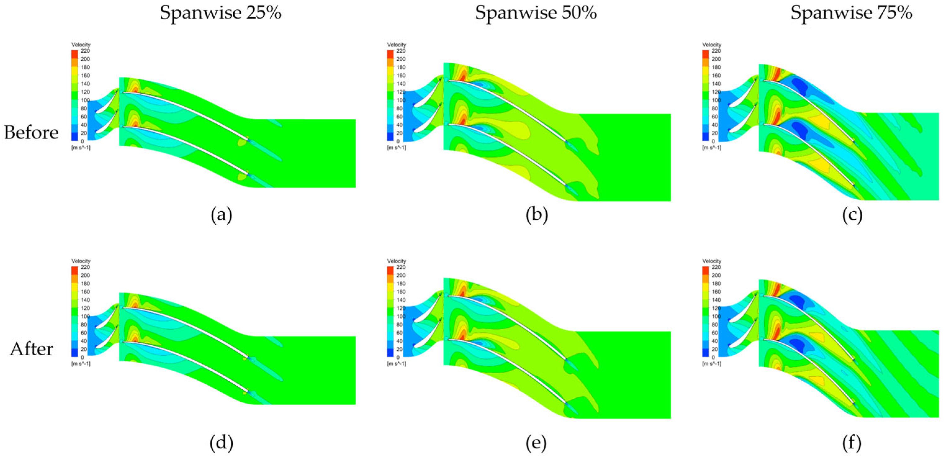
Figure 14 presents the velocity contour plots before and after optimization for the first-stage turbine. The plots represent the 25%, 50%, and 75% spanwise positions from left to right. In the rotor domain, a slight reduction in the low-speed region is observed. Significant changes in the velocity field are noted near the nozzle exit. To further examine these changes, Mach number contour plots were employed in
Figure 15. A substantial reduction in the regions with Mach numbers exceeding 1 is evident. This reduction indicates a decrease in losses through optimization, as regions with Mach numbers exceeding 1.0 are directly linked to losses in high-pressure-ratio applied turbines. For the second-stage turbine, similar to the first-stage turbine, subtle changes in the velocity field before and after optimization are observed, as depicted in
Figure 16. A more noticeable variation is observed in the temperature field. As shown in
Figure 17, a wider distribution of non-uniform temperature regions is identified before optimization. Lower temperatures signify increased production of shaft power in the turbine. However, in this case, the occurrence of lower temperatures, caused by reverse flow, leads to losses compared to the design point. Therefore, a uniform temperature decrease from the rotor inlet to the design exit temperature is deemed optimal. Based on these observations, it can be concluded that improvements have been achieved through optimization. Summarizing the qualitative analysis using pressure, temperature, and velocity, although the improvements are not dramatic, enhancements are evident in both turbines. However, it is important to note the limitations arising from the constrained adjustment range of design variables to minimize turbine shape variations, potentially preventing ideal optimization.
The results of this study, where changes were made to the radial turbine rotor’s hub and shroud profiles as well as the incidence angle while achieving a 1% or higher increase in the turbine’s total-to-total isentropic efficiency through numerical analysis, are significant. A 1% increase in turbine efficiency can have a substantial impact on the overall efficiency of an ORC power system that utilizes waste heat from the ship. This demonstrates the effectiveness of the optimization method using RBNN. When comparing the values of η
RBNN and η
CFD from
Table 9 and
Table 10, it is observed that the RBNN’s efficiency values are consistently higher than the results obtained through numerical analysis. The RBNN, although capable of approximating complex nonlinear functions, can be challenging to fully understand in terms of its exact computational process. Consequently, even when trained with CFD data, applying an RBNN-trained model to CFD simulations can yield slightly divergent results. This observed discrepancy represents a limitation in the application of the RBNN model in this research, emphasizing the need for further investigation in the future. Despite discrepancies between RBNN results and those from CFD simulations, RBNN has effectively approximated and captured the underlying data relationships, ultimately resulting in enhanced efficiency in the context of optimized design.


