Grid-Connected Phase-Locked Loop Technology Based on a Cascade Second-Order IIR Filter

Abstract

The moving average filter-based phase-locked loop (MAF-PLL) can obtain grid synchronization signals accurately under adverse grid conditions with a large amount of harmonics due to the high filtering capability of the MAF. However, MAF-PLL cannot achieve a fast dynamic response in the case of frequency drift, phase angle steps, and unbalanced voltage sag. MAF is essentially an FIR filter, and its filtering performance is hard to be adjusted. To address this issue, this paper proposes an alternative to MAF consisting of a set of cascading second-order IIR filters (CIIRF). Based on MAF, CIIRF introduces multiple zeros and poles from the zero–pole replacement perspective, and by changing the position of the poles, the filter performance can be adjusted. To improve the anti-interference ability of PLL based on CIIRF (CIIRF-PLL) in the presence of grid frequency drift, a frequency-adaptive scheme is also proposed. Simulation and experimental results show that CIIRF-PLL can accurately track the grid voltage phase in the case of frequency steps, phase angle jumps, harmonics injection, and unbalanced voltage sag and has good steady-state and dynamic performance.

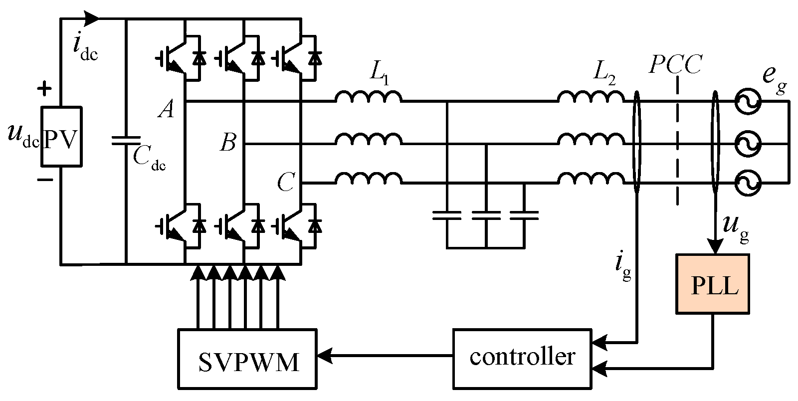
1. Introduction

The phase-locked loop (PLL) is widely used in a variety of real applications associated with signal synchronization and control of power electronic-based devices. With the increasingly growing usage of renewable energy sources such as wind and solar, grid-connected equipment and PLLs are of high importance [1,2,3,4]. Typically, the synchronous reference frame phase-locked loop (SRF-PLL) has been widely used due to its ease of operation and robust behavior under stiff grid conditions. However, under adverse grid conditions, a significant amount of unexpected ripple will appear. To improve the filtering capability in the weak grid, different in-loop low-pass filters have been incorporated into the SRF-PLL. For example, the SOGI [5,6,7], MAF [8,9,10], notch filter [11,12,13], linear Kalman filter [14], and delayed signal cancellation operator [15,16,17] can all be used to block the harmonics.

In-loop low-pass filters can be classified into two categories based on the harmonic elimination approach. The first type of filter is represented by SOGI, which may block high-frequency signals such as a phase-locked loop based on a double second-order generalized integrator (DSOGI-PLL) [18]. High-order harmonics can be efficiently suppressed by DSOGI-PLL, while low-order harmonics, such as the fifth and seventh harmonics, cannot be properly suppressed. A PLL based on multiple second-order generalized integrators (MSOGI-PLL) uses multiple SOGI modules in parallel to separate the fundamental component from each low-order harmonic through the control method that the output signals of each paralleled SOGI module feed forward to account for the weakening harmonics of the input voltage to a greater extent [19]. This method can prevent low-order harmonic interference, but it has a complex structure and significant system computation costs. Another type of filter, with MAF being the most common, performs fixed-point cleaning on each harmonic. Because of its simple digital realization and cheap computing overhead, a MAF operates as an excellent low-pass filter and is widely employed in many real-world implementations. In comparison to the first type of filter’s characteristics, the second type of filter is more extensively employed in practical applications.

The MAF-based phase-locked loop (MAF-PLL) incorporates a MAF into the SRF-PLL. It substantially rejects the harmonics and obtains an accurate synchronous grid voltage signal. The transient response, however, becomes slower due to the presence of the in-loop MAF. To address this issue, refs. [20,21] adopt a quasi-type-1 (QT1) PLL structure to compensate the delay, and [4] shorten the window length to 1/6 of the fundamental period, aiming to reduce the phase delay. However, only non-triple odd harmonics can be blocked. Authors [22,23,24] move the MAF out of the PLL as the prefilter, which provides a favorable dynamic performance but increases complexity and computational load. Another study [21] introduces a correction link and QT1 simultaneously into the feedback loop to improve the dynamic response. In [8], a phase-lead compensator (PLC) is used; however, the working mechanism and parameter selection of the PLC are not analyzed in detail.

Typically, adaptive schemes are used to improve the disturbance rejection capacity of the PLL when the grid voltage frequency varies [25,26,27]. To achieve the frequency adaptation, ref. [12] provides several frequency-adaptive schemes for the MAF-PLL and presents their simulation analysis, but the hardware implementation is not shown. In this paper, the round-to-nearest integer method is suggested.

Due to the fact that MAF-PLL is fundamentally a FIR filter and cannot achieve a quick dynamic response in the situation of frequency drift, phase angle step, and unbalanced voltage sag, its filtering performance is difficult to improve. This research suggests a set of cascading second-order IIR filters (CIIRF) as an alternative to MAF. From a zero–pole replacement standpoint, CIIRF introduces various zeros and poles based on MAF, and the filter performance may be altered by adjusting the pole positions. Additionally, a frequency-adaptive scheme is suggested to enhance the CIIRF-PLL’s anti-interference performance in the presence of grid frequency drift.

This paper is organized as follows: In Section 2, the standard MAF is analyzed, and a structure diagram of the standard MAF-PLL is given. In Section 3, the proposed method is presented along with an analysis of its performance. Section 4 presents the design guidelines for the system parameters. Section 5 suggests the frequency-adaptive method and shows the hardware implementation. Finally, in Section 6, simulation and experimental results are shown to validate the feasibility and effectiveness of the proposed method.

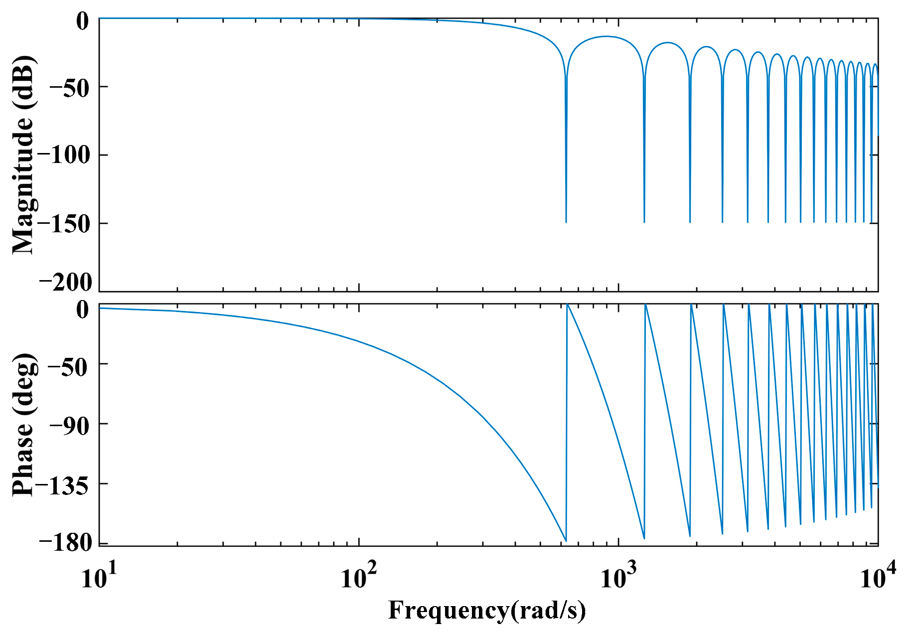
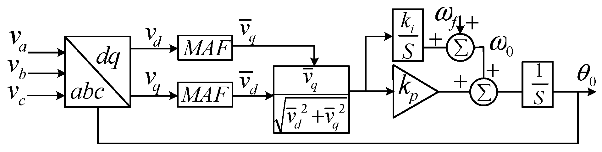
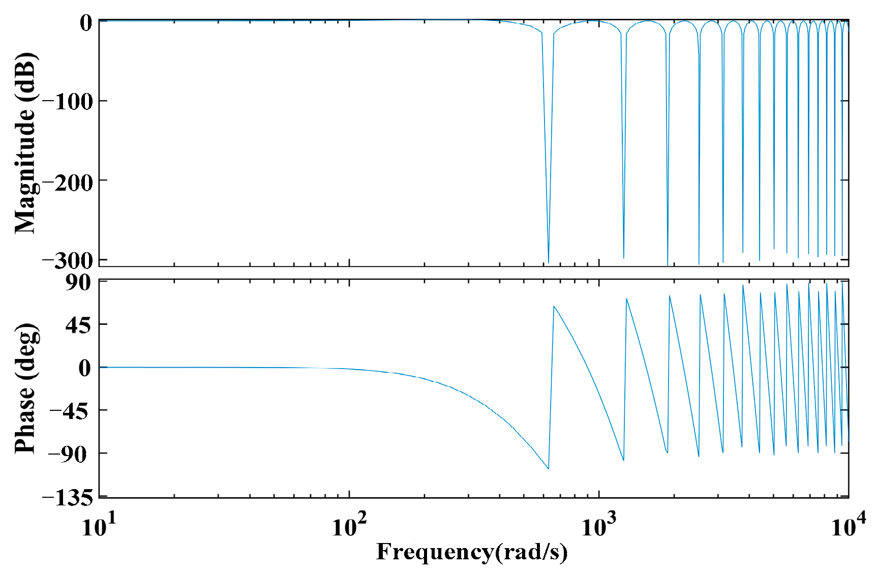
2. Analysis of the Standard MAF-PLL

Figure 1 shows the system structure of the grid-connected inverter with an LCL filter. To obtain a reliable grid connection at the point of common coupling (PCC), the synchronization signal of the grid voltage must be extracted. Typically, SRF-PLL is widely used under a stiff grid condition. However, when the grid voltage is distorted due to significant harmonic pollution, the SRF-PLL is unable to obtain the synchronization signal correctly. To address the issue, one possible solution is to introduce a MAF into the SRF-PLL to eliminate the harmonic disturbance.

The transfer function of the standard MAF can be expressed in the s-domain [14].

$$G_{\mathrm{MAF}}(s)=\frac{1-{\mathrm{e}}^{-T_{\mathrm{w}}s}}{T_{\mathrm{W}}s}$$

(1)

where T_w is the window length. Assuming that T_s is the control system sampling time, the window length T_w contains N sample, and N = T_w/T_s. It is worth noting that the selection of the window length T_w is decided by the grid’s harmonic components, and it is recommended that T_w = T (nominal grid period) in the case that the grid’s harmonic components are uncertain, or T_w = T/2 and T_w = T/6, respectively, in the case that the odd harmonics and the non-triple odd harmonics are present in the applications [16]. According to the harmonic components, the window length T_w = T/2 is considered in this paper.

The Bode plot of MAF is presented as follows.

From Figure 2, it can be observed that the MAF has a set of notches centered at 1/T_w in hertz and its integer multiples, which act as a quasi-ideal low-pass filter. The MAF provides unity gain at zero frequency and negative gain at notch frequencies n/T_w (n = 1, 2, 3, …) in hertz. This means passing the dc component and completely blocking the frequency components of the integer multiples of 1/T_w in hertz.

Based on the filtering characteristics analyzed earlier, MAF is introduced into the SRF as an in-loop filter. The structure diagram and small-signal model of MAF-PLL are given as follows.

Figure 3 shows the structure of the MAF-PLL, which includes two in-loop MAFs and an SRF-PLL. To reduce the negative effect of the input voltage amplitude variation on the PLL, an amplitude normalization scheme (ANS) is also incorporated into the PLL.

The bode plot of the open-loop transfer function of the standard MAF-PLL is shown in Figure 4. The parameters of the proportional integrator are k_p = 83.33 and k_i = 2893.5. The magnitude margin is 14.1 dB and the phase margin is 43.3°; this means that the MAF-PLL is stable. The cut-off frequency ω_c, on the other hand, is insufficiently high, resulting in a slow dynamic response.

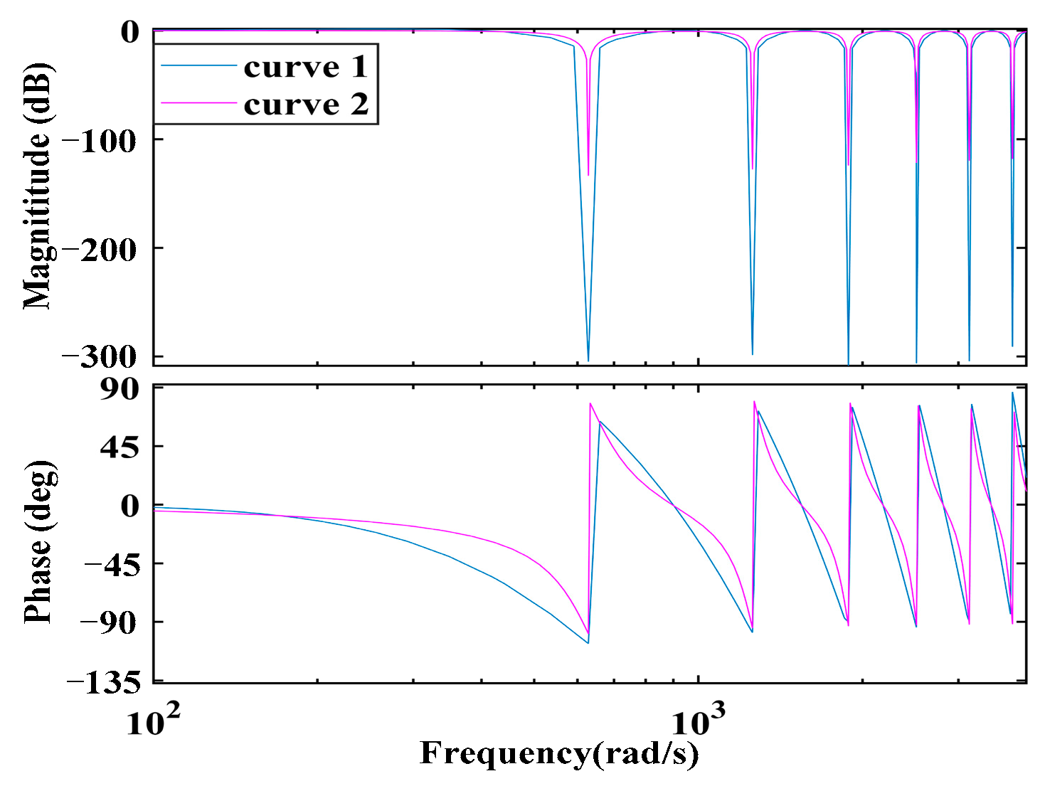
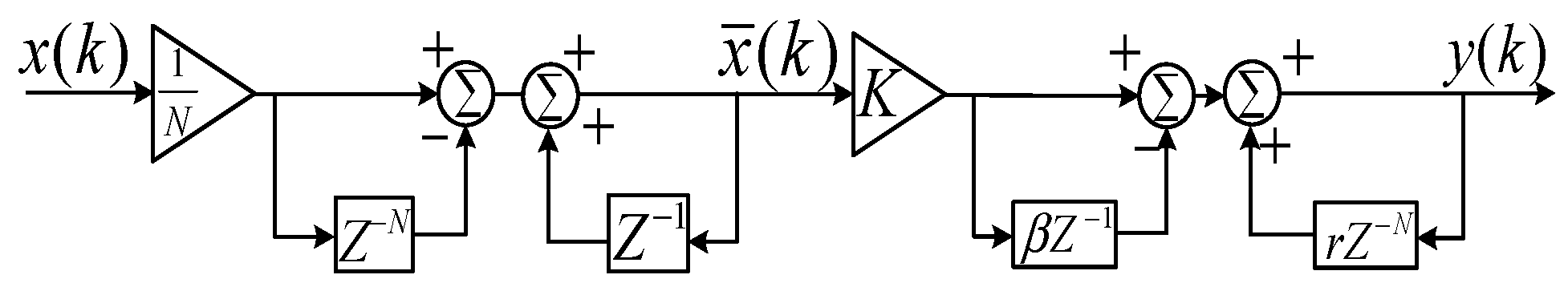
3. The Proposed Method

The standard MAF-PLL suffers from a slow dynamic response due to the presence of the in-loop MAF. Examining Figure 4, in order to increase the cut-off frequency of the standard MAF-PLL, and, thus, improve the dynamic performance, the proportion coefficient k_p of the PI regulator could be increased. However, looking at the phase–frequency characteristics in Figure 4, it can be seen that too much phase lag will lead to insufficient phase margin and system instability. Therefore, phase compensation becomes a key issue.

Analyzing the frequency characteristic in Figure 2, it can be seen that the magnitude attenuation occurs at the frequencies except for the notch frequencies n/T_w (n = 1, 2, 3…) in hertz and many high-frequency signals are filtered; this is the essence of the phase delay. Consequently, the phase delay can be reduced by increasing the amplitude–frequency gain in the passband.

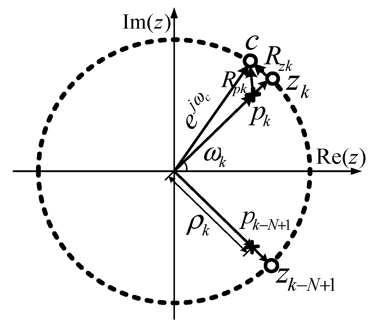
3.1. Zero–Pole Replacement

If the nonlinear delay term $e^{-T_{\mathrm{w}}s}$ in Equation (1) is linearized using the first-order Pade approximation expressed as Equation (2), Equation (3) is easily obtained:

$$e^{-T_{\mathrm{w}}s}\approx \frac{1-T_{\mathrm{W}}s/2}{1+T_{\mathrm{W}}s/2},$$

(2)

$$G_{\mathrm{MAF}}(s)\approx \frac{1}{T_{\mathrm{W}}s/2+1}.$$

(3)

From Equation (3), it is noted that the MAF provides approximate unity gain in the low-frequency region (below the fundamental frequency) and large attenuation at the frequencies in the high-frequency region, which matches the magnitude–frequency character in Figure 2. According to the analysis above, with the aim of improving the frequency gain at the passband, the first correction link G_c1(s) that has only one zero is introduced, and its transfer function is given as follows:

$$G_{\mathrm{c}1}(s)=\frac{T_{\mathrm{W}}s}{2}+1,$$

(4)

$$G_{\mathrm{c}1}\left(s\right)G_{\mathrm{MAF}}\left(s\right)\approx 1.$$

(5)

Figure 5 shows the Bode plot of G_c1(s)G_MAF(s) after adding the correction link G_c1(s), which introduces a zero into the original filter. Compared with Figure 2, the amplitude–frequency gain at the passband in the high-frequency region almost achieves 0 dB, and the phase also improves. The gain at the vicinity of the notch frequencies is not flat enough, which also affects the dynamic performance. One possible way of obtaining flatter gain at the passband is to fine-tune the amplitude–frequency gain by adjusting the quantity and position of the poles.

To better discuss the phase compensation scheme from the zero–pole replacement perspective, it is preferable to analyze the system in the z-domain. By discretizing the MAF, the transfer function in the z-domain can be obtained:

$$G_{\mathrm{MAF}}(z)=\frac{1-{\mathrm{z}}^{-N}}{N}\cdot \frac{1}{1-z^{-1}}=\frac{1}{N}{\displaystyle \prod _{K=1}^N\frac{z-z_k}{z-p_1},}$$

(6)

where N denotes the sample order.

It can be observed from Equation (6) that there are N zeros on the unit circle and one pole fixed at the origin. Consequently, the MAF is essentially an FIR filter with a linear phase–frequency curve whose drawback is that its performance cannot be tuned by changing the position of its poles because it only has a fixed pole at the origin. For the purpose of system adjustment, N poles will be introduced. Furthermore, for system stability, all introduced poles should be located in the unit circle. Therefore, a second correction link G_c1(s) that has only poles is given as follows:

$$G_{\mathrm{c}2}(s)=\frac{1}{1-r{\mathrm{e}}^{-T_{\mathrm{w}}s}},$$

(7)

where the parameter $r\in \left[0,1\right)$ denotes the attenuation factor at the notch frequencies. Similarly, Equation (7) can be rewritten as Equation (8) by approximating the delay term $e^{-T_{\mathrm{w}}s}$ using the first-order Pade approximation expressed as Equation (2).

$$G_{\mathrm{c}2}(s)=\frac{1+T_{\mathrm{W}}s/2}{(1-r)+(1+r)T_{\mathrm{W}}s/2}=\frac{G_{\mathrm{c}1}\left(s\right)}{(1-r)+(1+r)T_{\mathrm{W}}s/2}.$$

(8)

Noted that the correction link G_c1(s) is included in Equation (8), we can use the correction link G_c2(s) instead of G_c1(s). Equation (9) can be obtained by multiplying Equation (8) with Equation (4).

$$G_{\mathrm{c}2}(s)G_{\mathrm{MAF}}(s)=\frac{1}{(1-r)+(1+r)T_{\mathrm{w}}s/2}.$$

(9)

From Equation (9), after adding G_c2(s), another pole arises. To ensure that the amplitude–frequency gain of G_c1(s)G_MAF(s) at the passband is equal to 0 dB, G_c2(s) is modified into G_c(s) as Equation (10).

$$G_{\mathrm{c}}(s)=\frac{(1-r)+(1+r)T_{\mathrm{W}}s/2}{1-r{\mathrm{e}}^{-T_{\mathrm{W}}s}}.$$

(10)

By discretizing Equation (10) and doing some simple mathematical operations, the discrete expression can be neatly given as Equation (11):

$$G_{\mathrm{c}}(z)=K\frac{1-\beta {\mathrm{z}}^{-1}}{1-r{\mathrm{z}}^{-N}},$$

(11)

where

$$K=\frac{N}{2}(1+r)+(1-r),$$

$$\beta =\frac{N(1+r)}{N(1+r)+2(1-r)}.$$

For a given N and r, K and β are both constant. After introducing some zeros and poles synthesized in G_c(s), the transfer function of G_CIIRF(z) can be obtained as

$$\begin{array}{l}{G}_{\mathrm{CIIRF}}\left(z\right)=G_{\mathrm{MAF}}\left(z\right)G_{\mathrm{c}}\left(z\right)\\ \hspace{1em}\hspace{1em}\hspace{1em}\hspace{0.33em}\hspace{0.33em}=\frac{1-{\mathrm{z}}^{-N}}{N(1-z^{-1})}\frac{K(1-\beta {\mathrm{z}}^{-1})}{1-r{\mathrm{z}}^{-N}}=\frac{K}{N}{\displaystyle \prod _{k=0}^N\frac{z-z_k}{z-p_k}}\end{array}$$

(12)

It is easily seen from Equation (12) that in the complex z-plane, there exist N + 1 zeros on the unit circle and poles of the same quantity in the circle.

$$Z_k=e^{j2\pi (k{f}_S/N)},\hspace{1em}k=0,\hspace{0.17em}1,\hspace{0.17em}2,\cdots ,\hspace{0.17em}N,$$

(13)

$$P_k=\sqrt[N]{r}\cdot e^{j2\pi (k{f}_S/N)},\hspace{1em}k=0,\hspace{0.17em}1,\hspace{0.17em}2,\cdots ,\hspace{0.17em}N.$$

(14)

Through some mathematical operations on Equation (12), the following is obtained:

$$\begin{array}{l}{G}_{\mathrm{CIIRF}}(z)=\frac{K(1-\beta {\mathrm{z}}^{-1})}{N(1-z^{-1})}\frac{1-z^{-N}}{1-r{z}^{-N}}\\ \hspace{1em}\hspace{1em}\hspace{1em}\hspace{0.17em}\hspace{0.33em}=\underset{f_{g\hspace{0.33em}}gain}{\underbrace{\frac{K(1-\beta {\mathrm{z}}^{-1})}{N(1-z^{-1})}}}\cdot \underset{harmonics\hspace{0.17em}rejection}{\underbrace{{\displaystyle \prod _{K=1}^{N/2}{G}_k\left(z\right)}}},\end{array}$$

(15)

where

$$G_k(z)=\frac{(z-z_k\left)\right(z-z_{N-k+1})}{(z-p_k\left)\right(z-p_{N-k+1})}$$

(16)

It is noted that G_CIIRF(z) is the proposed alternative filter of MAF in this paper, i.e., CIIRF, which is divided into two parts. The first part represents the tracking gain at the fundamental frequency, and the second part consists of a set of second-order IIR filters expressed as Equation (16), which is responsible for the harmonic rejection. Curve 2 in Figure 6 depicts the Bode plot of G_CIIRF(z) (r = 0.99).

For better visualization, the Bode plot in Figure 5 is redrawn as Curve 2 in Figure 6. Curve 2, that is, the frequency characteristic curve of G_CIIRF(z), has a flatter passband when compared with Curve 1, but with a smaller negative gain at the notch frequencies. This is, however, sufficient for harmonic suppression and has a larger phase in the low frequency region although the phase–frequency characteristic is slightly nonlinear; this is negligible in this application. It can be concluded that CIIRF, such as the IIR filter, has adjustable poles that can fine-tune the amplitude–frequency gain and phase of the filter, thus adjusting the performance of the filter. Next, CIIRF will be further discussed.

Figure 7a depicts the open-loop Bode plot of G_CIIRF(z) with different values of the parameter r. The enlarged plot in Figure 7b shows that G_CIIRF(z) provides the flatter magnitude response at the passband. Moreover, the 3 dB bandwidth at the notch frequencies decreases with an increase in parameter r, which provides a flat magnitude response at the passband; hence, it improves the transient performance. However, the attenuation at the notch frequencies decreases with an increase in parameter r. To achieve a better performance tradeoff between the flatter magnitude response at the passband and more sufficient attenuation at the notch frequencies by adjusting the value of parameter r, one possible solution is to minimize the filter gain–bandwidth product at the notch frequencies [28].

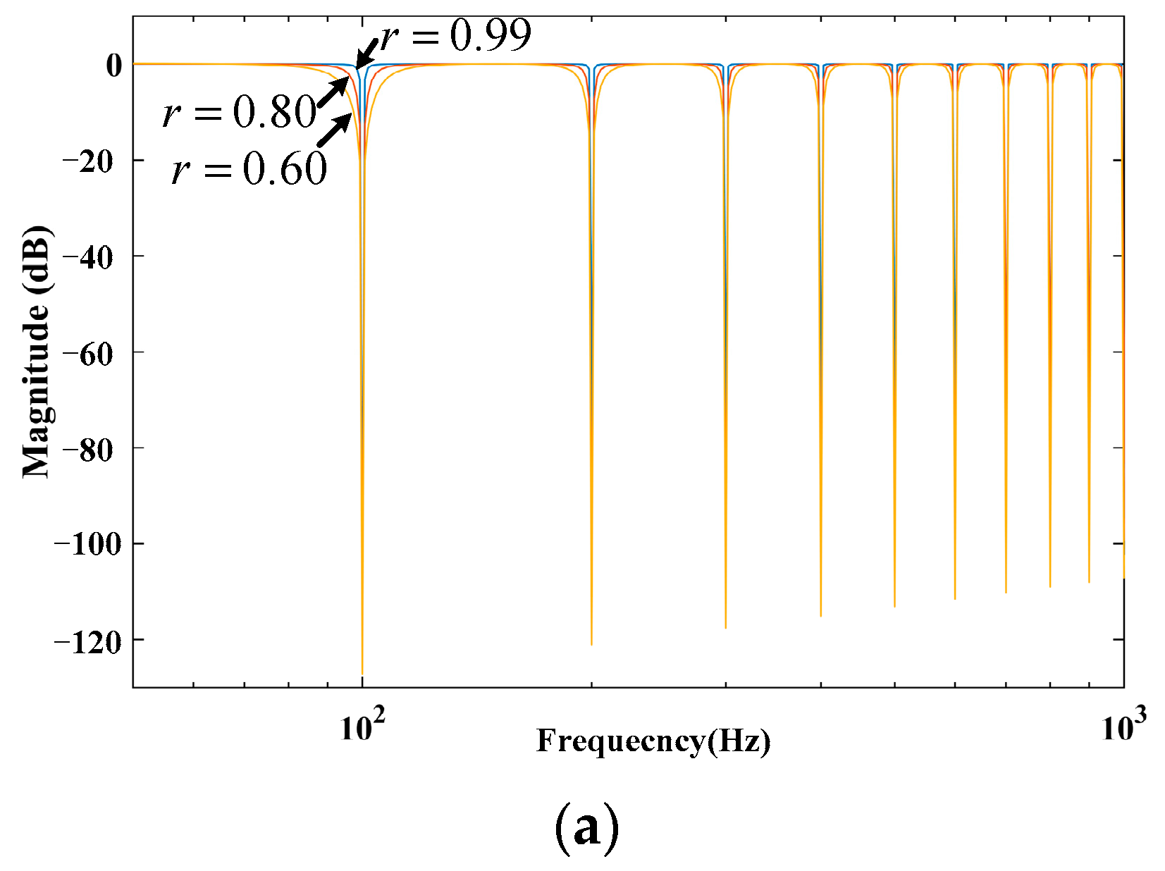
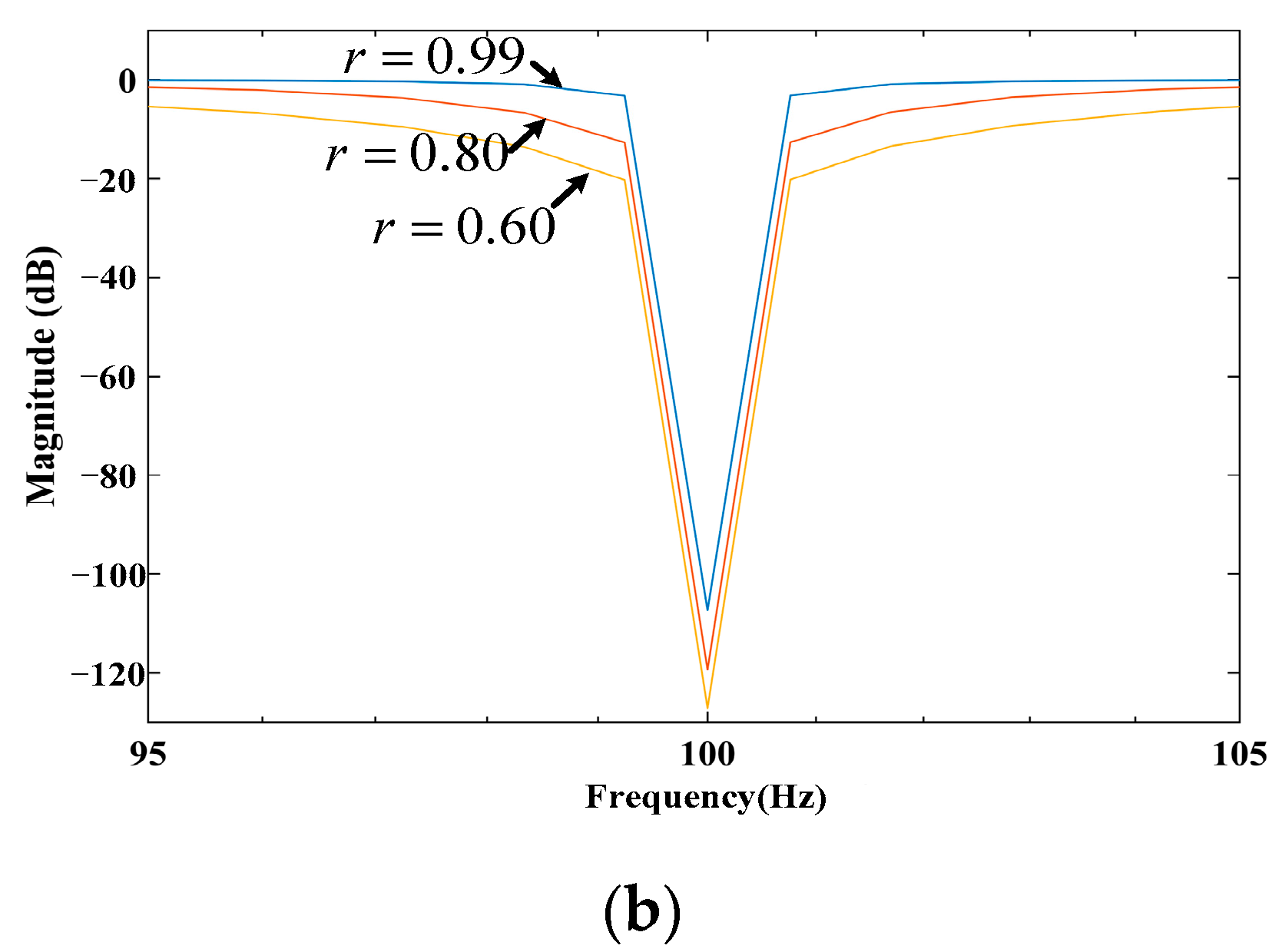
3.2. Selection of Parameter r

By converting Equation (16) into another form, the following is obtained:

$$G_k(z)=\frac{1+a_k{z}^{-1}+z^{-2}}{1+{\rho }_k{a}_k{z}^{-1}+{\rho }_k^2{z}^{-2}},$$

(17)

$${\omega }_k={\cos }^{-1}(-a_k/2)rad,\hspace{0.33em}\hspace{0.17em}\hspace{1em}-2<a_k<2,$$

(18)

$$B{W}_{\mathrm{n}}=\pi (1-{\rho }_k)rad,\hspace{0.17em}\hspace{0.17em}\hspace{1em}{\rho }_k=\sqrt[N]{r}<1,$$

(19)

where the tuning parameters $a_k$ and ${\rho }_k$ are related to the normalized center frequency ω_k and the normalized bandwidth BW_n at the notch frequencies, respectively.

Figure 8 shows the pole–zero plot of the second-order IIR filter G_k(z) shown in Equation (17). Two pole–zero pairs are of mirrored layout in the z-plane. The pole–zero pair lying in the upper half of the z-plane is mapped to the real frequency in the frequency domain, i.e., the harmonic frequency.

Assuming that c is an arbitrary point on the unit circle that is in close vicinity of the zero Z_k that corresponds to the line frequency ω_k, the gain of G_k(z) at point c on the unit circle that corresponds to the line frequency ω_c can be obtained by substituting the $z=e^{\mathrm{j}{\omega }_{\mathrm{c}}}$ into Equation (17) and calculating the amplitude of G_k($e^{\mathrm{j}{\omega }_{\mathrm{c}}}$). The further the distance between point c and zero Z_k, the larger the attenuation gain of G_k(z) at point c for a fixed pole P_k or ${\rho }_k$. However, for a fixed point c, tuning the position of the pole P_k can regulate the gain and phase of G_k(z), thus improving system performance. When moving point c infinitely close to the zero Z_k, the difference R_zk between the vector Z_k and $e^{{\mathrm{j}\omega }_{\mathrm{c}}}$ approaches $\epsilon$ which is a infinitesimal constant. The ratio of the vectors R_zk and R_pk is the difference between the vectors P_k and the vector $e^{\mathrm{j}{\omega }_{\mathrm{c}}}$ and is approximately equal to $\epsilon /\left(1-{\rho }_k\right)$, which represents the gain of G_k($e^{\mathrm{j}{\omega }_{\mathrm{c}}}$) at the point c. However, from the attenuation point of view, the decay multiple is equal to the reciprocal of the gain, i.e., $\left(1-{\rho }_k\right)/\epsilon$. According to the aforementioned analysis, for simplicity, the filter gain–bandwidth product at the notch frequencies is represented by the product of the bandwidth and decay multiple, as shown in Equation (20):

$$G=\pi (1-{\rho }_k)\cdot (1-{\rho }_k)/\epsilon =\pi (1-{\rho }_k{)}^2/\epsilon .$$

(20)

The minimization of the filter gain–bandwidth product at the notch frequencies is equivalent to minimizing the value of the expression G by tuning the parameter ${\rho }_k$. When ${\rho }_k$ comes infinitely close to 1, i.e., $\sqrt[\mathrm{N}]{r}\approx 1$, expression G takes the minimal value. Taking processing unit resolution into account, it is assumed that ${\rho }_k=0.9999$, then $r=0.99$ when N = 100.

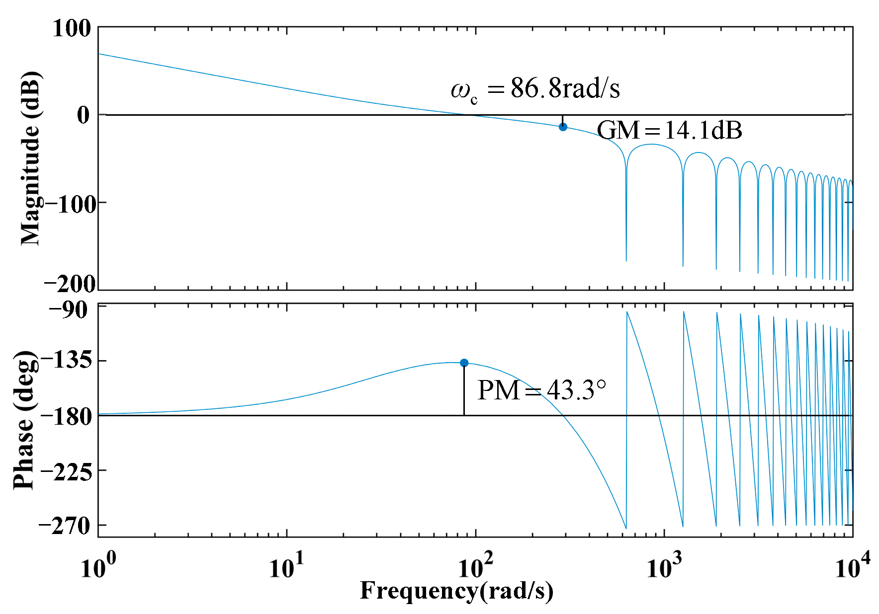
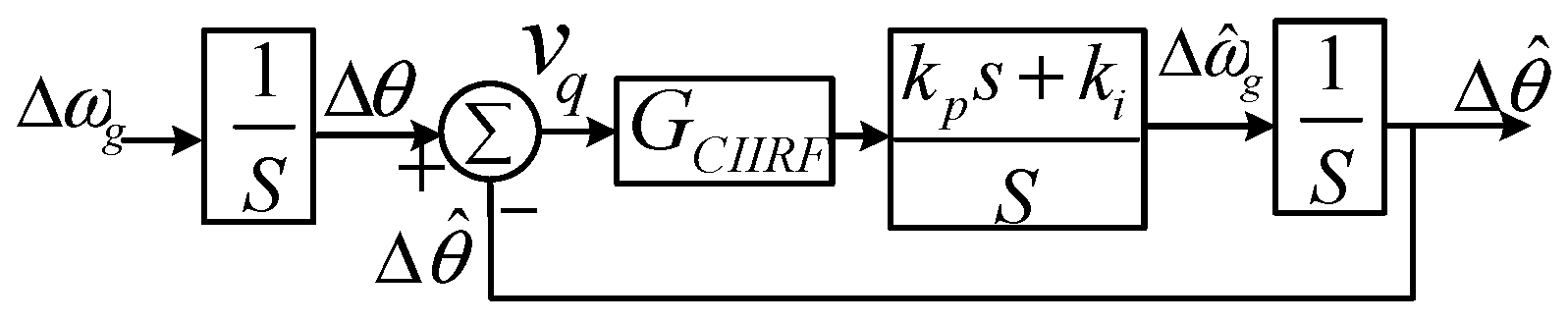
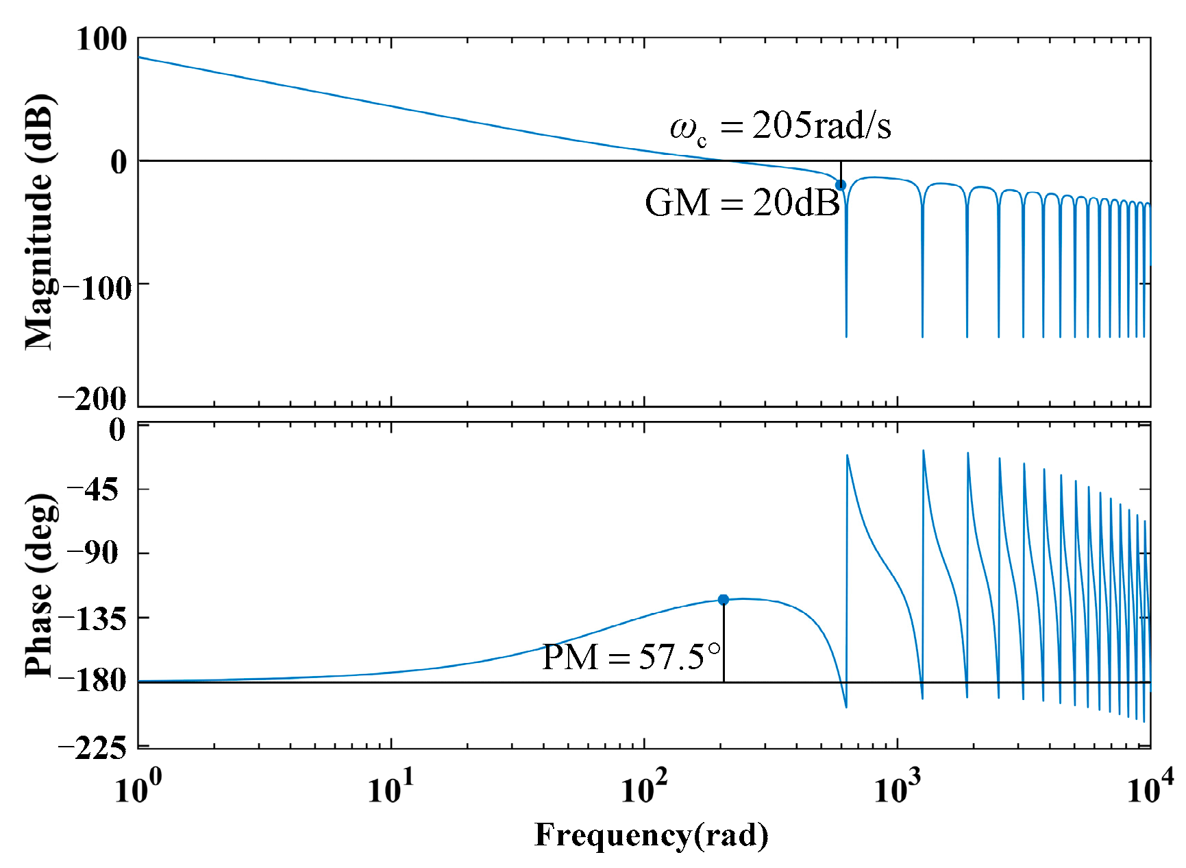
4. PI-Type Controller Parameter Design

Some controller design guidelines for the PLL are presented in this section. This paper proposes the replacement of MAF in Figure 3 with the CIIRF. Therefore, as shown in Figure 9, the small-signal model of the CIIRF-based PLL can be obtained by referring to Figure 3.

According to this model, the open-loop transfer function of CIIRF-PLL can be obtained as

$$G_{ol}(s)=G_{\mathrm{CIIRF}}\frac{k_{p}s+k_i}{s^2}.$$

(21)

As seen in Figure 7, the IIIRF with ${\rho }_k=0.9999$ provides almost unity gain at the passband. Therefore, GIIIRF is approximately equal to one and can be neglected. The close-loop transfer function of CIIRF-PLL can be obtained.

$$G_{cl}(\mathrm{s})=\frac{G_{ol}(\mathrm{s})}{1+G_{ol}(\mathrm{s})}\approx \frac{k_{p}s+k_i}{s^2+k_{p}s+k_i}$$

(22)

It is easily observed that Equation (22) is a typical second-order system. In contrast to the common expression of a typical second-order system, $k_p=2\zeta {\omega }_n$ and $k_i={\omega }_n^2$, where ${\omega }_n$ and $\zeta$ are the natural frequency and damping factor, respectively. To achieve the best damping effect and a fast transient response, $\zeta =0.707,{\omega }_n=2\pi 20 \mathrm{rad}/\mathrm{s}$, $k_p=177.71,k_i$ = 15,791.

Figure 10 shows the close-loop Bode plot of the proposed CIIRF-PLL. Compared with the close-loop Bode plot of the MAF-PLL in Figure 4, the magnitude and phase margin increase considerably; moreover, the bandwidth improvement more than doubles.

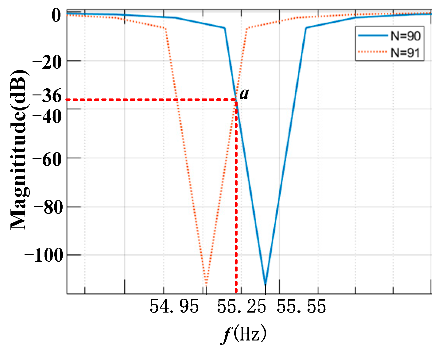
5. Frequency-Adaptive CIIRF Implementation

The CIIRF-PLL can block the sinusoidal disturbance of integer multiples of the frequency f_d which is twice the nominal frequency when T_w = 0.01, and the grid fundamental frequency keeps the nominal value unchanged. However, the CIIRF-PLL cannot completely block the disturbance components due to the variation in the disturbance frequency f_d with the grid fundamental frequency. Therefore, a frequency-adaptive CIIRF-PLL structure (FACIIRF-PLL) is proposed in this paper. To achieve frequency–adaptive performance, many online adjustment approaches are provided in the earlier literature [10].

According to the expression of the sample order N = f_s/f_d, one possible method is to keep the N constant by adjusting the system sample frequency adaptively to the grid frequency variations. It is worth noting that, in most cases, changing the system sample frequency will deteriorate the system control strategy; thus, adjusting the sample frequency adaptively is not feasible. The authors of [28] proposed that N can vary adaptively to the grid frequency variations according to the estimated grid frequency; this is associated with different detailed approaches found in the earlier literature. The sample order N can be adjusted via the rounding-down, rounding-up, rounding-to-nearest integer, weight mean value, and linear interpolation methods. Contrary to the round-to-nearest integer method, the rounding-down and rounding-up methods produce greater error, but they are easier to be implement on digital hardware. The weighted mean value and linear interpolation methods can provide less error; however, they cause greater calculation load on the processor in digital implementation. Therefore, considering the tradeoff, the round-to-nearest integer method is a relatively good option.

According to the aforementioned analysis, the notch center frequency of FACIIRF is determined by the value of N corresponding to the variant estimated frequency. The estimated frequency within a certain range matches the same N because the value of N is attained by using the round-to-nearest integer method. For example, assuming that N = 90 or N = 91, the estimated frequency ranges are approximately $\left(55.55\pm 0.3\right)$ Hz and $\left(54.95\pm 0.3\right)$ Hz, respectively, which are shown in Figure 11.

From Figure 11, it can be seen that intersection a represents the critical frequency, and its corresponding gain is approximately −36 dB. The closer to the center frequencies the estimated frequency is, the larger the attenuation gain.

The first row of Table I lists the distortion limits in IEEE Standard 519-2014 [29]. The second row lists a given worse case of grid voltage distortion, which is far beyond the distortion limits listed in the first row. When the fundamental frequency of the given grid voltage drifts to the intersection a shown in Figure 11, each individual harmonic will be attenuated by 36 dB adopting the FACIIRF. After filtering, the data related to harmonic distortion are listed in the third row of

Table 1. Harmonic distortion list.

Harmonic Order h	h < 11	11 ≤ h and h < 17	17 ≤ h and h < 23	23 ≤ h and h < 35	h ≥ 35	Total Distortion
Distortion Limits	4.0%	2.0%	1.5%	0.6%	0.3%	5.0%
Voltage harmonics	30%	5%	0	0	0	35%
After Filtering	0.47%	0.08%	0	0	0	0.55%

. The total distortion is far below that in the first row. Therefore, the FACIIRF is also applicable under the most unfavorable conditions in practical applications.

Figure 12 shows the digital implementation schematic diagram of CIIRF, which is described by the difference equation, i.e., Equation (23).

$$\left\{\begin{array}{l}\overline{x}(k)=\frac{1}{N}\left[x(k)-x(k-N)\right]+\overline{x}(k-1)\\ y(k)=r\cdot y(k-N)+K\cdot \overline{x}(k)-K\cdot \beta \cdot \overline{x}(k-1)\end{array}\right.,$$

(23)

where $x\left(k\right), y\left(k\right)$ are the input and output variables, respectively, and $\overline{x}\left(k\right)$ is intermediate variable.

6. Simulation Analysis and Experimental Result

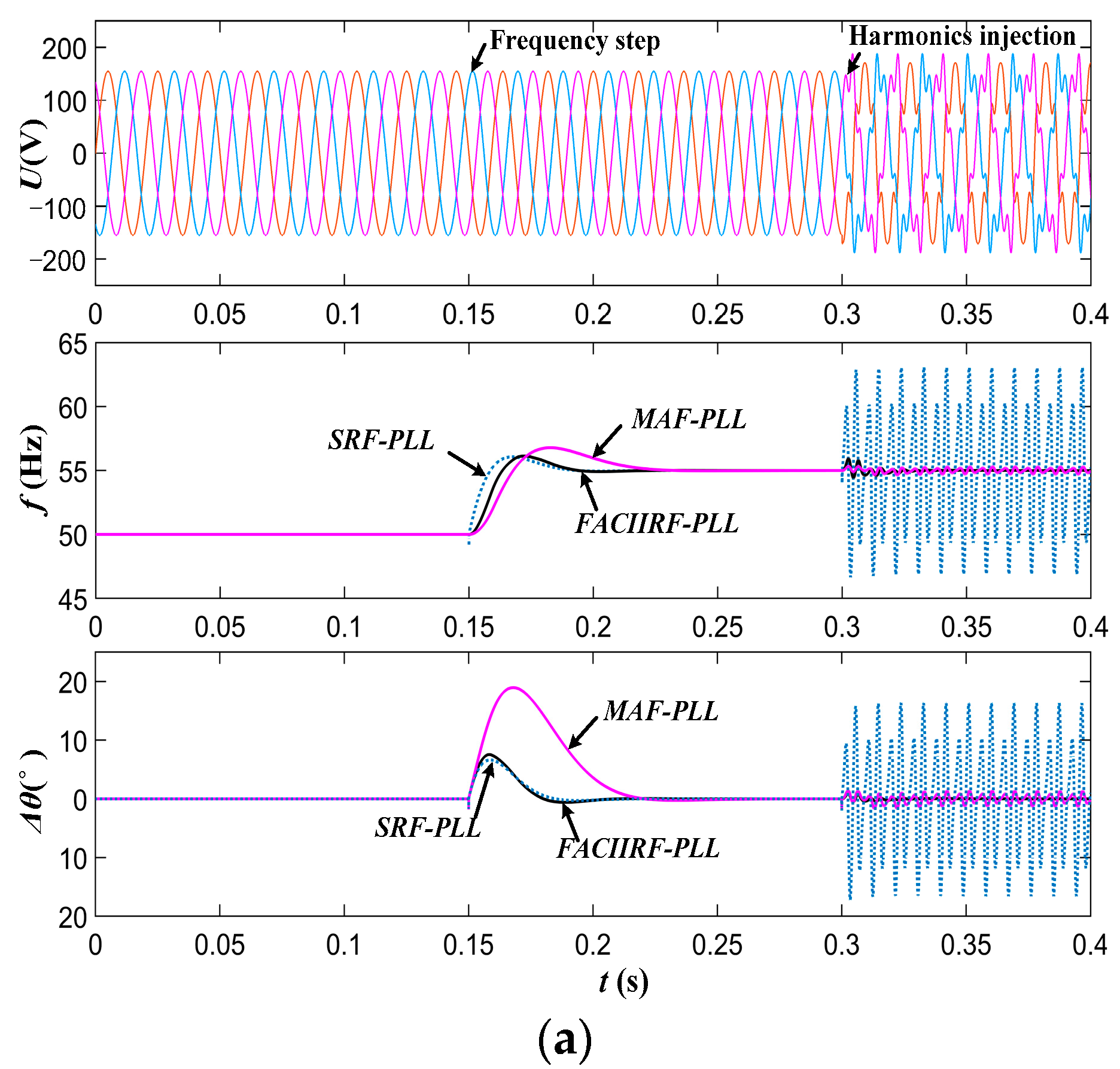
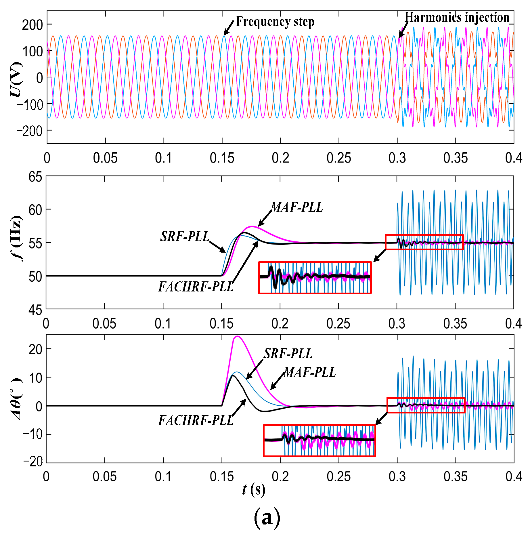
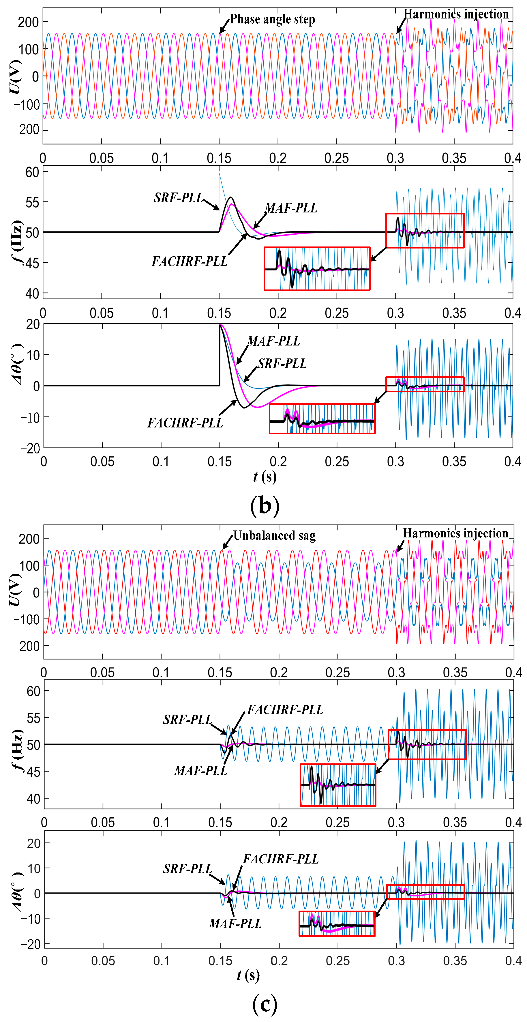
6.1. Simulation Analysis

Simulations are implemented in the Matlab/Simulink environment to analyze the effectiveness of the proposed PLL structure in this section. To highlight the effectiveness of the proposed method, some comparative analysis will be completed with the conventional SRF and standard MAF, where the control parameter designs of the latter two are carried out using the symmetrical optimum method.

To investigate the stability and dynamic performance of the proposed FACIIRF-PLL, three different operating cases will be provided, which, respectively, represent the frequency step, phase angle jump, and unbalanced sag followed by harmonic injection. The specific description is as follows:

• Case 1: The grid voltage undergoes a frequency step change of +5 Hz at time 0.15 s and injection of 0.2 pu for the 5th harmonic, 0.1 pu for the 7th harmonic, and 0.05 pu for the 11th harmonic at time 0.3 s.
• Case 2: The grid voltage undergoes a phase angle jump of +20° at time 0.15 s and an injection of 0.2 pu for the 5th harmonic, 0.1 pu for the 7th harmonic, and 0.05 pu for the 11th harmonic at time 0.3 s.
• Case 3: The grid voltage undergoes an A-phase amplitude drop of 0.3 pu at time 0.15 s and an injection of 0.2 pu for the 5th harmonic, 0.1 pu for the 7th harmonic, and 0.05 pu for the 11th harmonic at time 0.3 s.

The simulation results of the three PLLs under Case 1 are shown in Figure 13a. When the grid voltage undergoes a frequency step of +5 Hz at 0.15 s, the frequency error and phase angle error of SRF-PLL and FACIIRF-PLL both reach zero much faster than those of MAF-PLL. As to the frequency and phase angle errors, when the harmonics are injected into the grid voltage at 0.3 s, SRF-PLL produces a violent oscillation so as not to reach zero, and MAF-PLL fluctuates slightly in the vicinity of zero while FACIIRF-PLL can approach zero soon.

The simulation results of the three PLLs under Case 2 are shown in Figure 13b. When the grid voltage undergoes a phase angle step of +20° at 0.15 s, the frequency error of FACIIRF-PLL is faster to reach zero than that of MAF-PLL but is a bit slower than that of SRF-PLL. The phase angle error of FACIIRF-PLL reaches zero as fast as that of SRF-PLL, but much faster than that of MAF-PLL. When harmonics are injected into the grid voltage at 0.3 s, SRF-PLL produces a violent oscillation so that the frequency error and phase angle error cannot reach zero, while those of MAF-PLL and FACIIRF-PLL can both approach zero soon.

The simulation results of the three PLLs under Case 3 are shown in Figure 13c. When the grid voltage experiences an unbalanced sag at 0.15 s and harmonics injection at 0.3 s, the frequency and phase angle errors of FACIIRF-PLL reach zero as quickly as those of MAF-PLL, whereas those of SRF-PLL vibrate and cannot converge.

To sum up, among the three PLLs, the FACIIRF-PLL improves the dynamic response speed while ensuring that the phase is locked accurately.

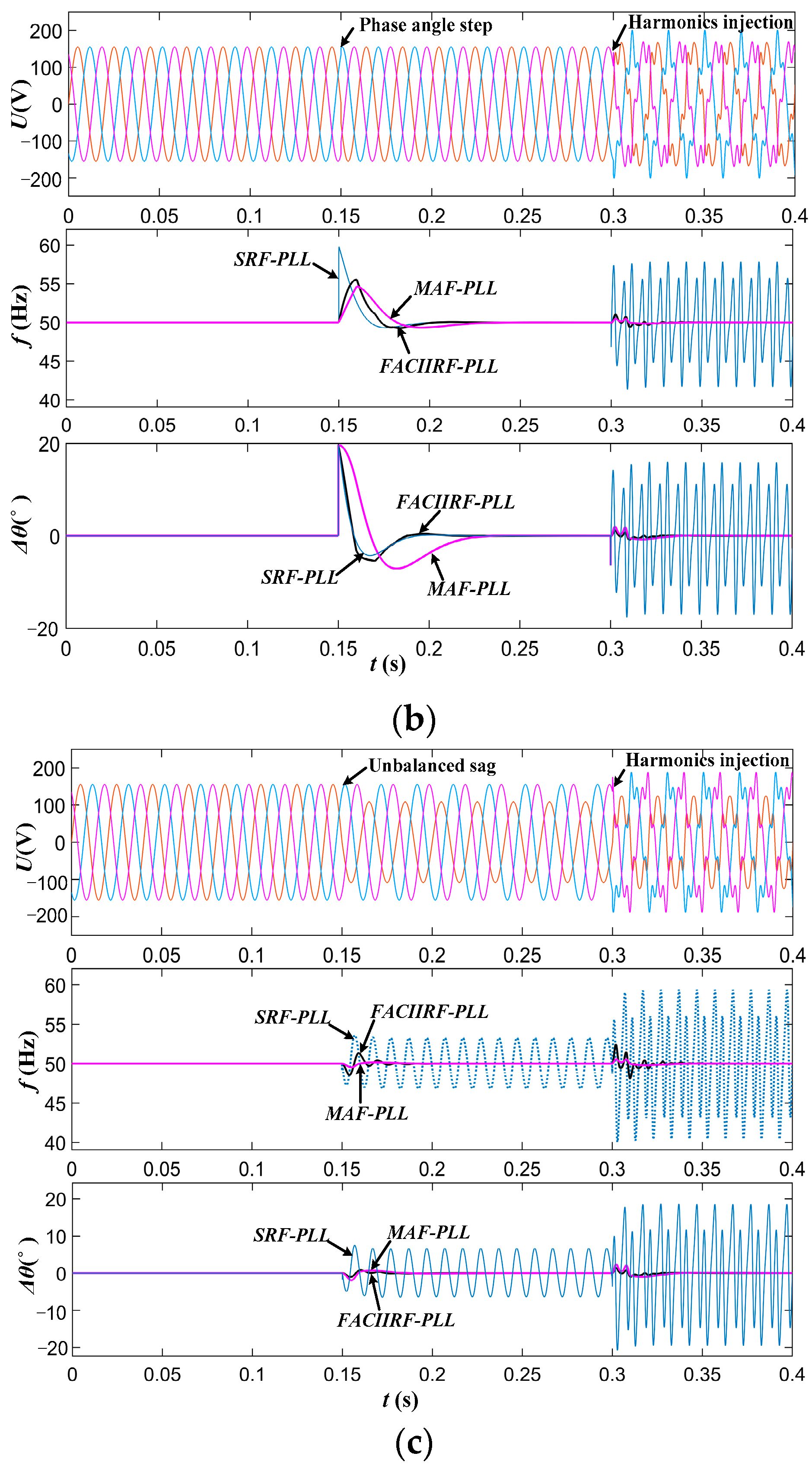
6.2. Experimental Results

In this section, the effectiveness and hardware implementation of the proposed method are validated. In this experiment, a set of experimental devices for detecting the grid voltage synchronization signal are used. The main control processor is the TMS320F28335 digital signal processor of the TI company, which realizes the digital operation of the algorithm. For simplicity, three different operating cases associated with the grid voltage signal are generated by the same control processor. They are implemented by code placed in the interrupt program, which can avoid the impact of sampling errors on the verification results. The sampling frequency of the DSP is set to 10 kH. In addition, the waveform data generated in the experiment are transmitted to the upper computer software through cache and serial port communication, then the graphics are drawn. Figure 14 shows the experimental devices used in experiments. The three working conditions set in the experiment are consistent with those in the simulation, and the waveforms of various PLLs are shown in Figure 15.

It can be seen from Figure 15 that the experimental waveforms of the phase angle error and frequency error of the three PLLs under three different operating cases are almost consistent with the simulation results.

Under the test condition of harmonic injection after the frequency step, phase angle jump, and unbalanced sag, the frequency dynamic response of the SRF-PLL is fastest among the three PLLs, but the waveforms of the frequency error and phase error vibrate under the cases of unbalanced sag and harmonic injection. In the following discussion, some performance comparisons between MAF-PLL and FACIIRF-PLL are made.

In Figure 15a, in the case of the frequency step and compared with the frequency tracking performance of MAF-PLL, FACIIRF-PLL is about 30 ms faster and has a little less overshoot; compared with the phase tracking performance of MAF-PLL, FACIIRF-PLL reaches the stable state with a significantly smaller overshoot and faster speed. It is obvious that after the harmonics are added at 0.3 s, the waveform of FACIIRF-PLL achieves the stable state quickly, while the waveform of MAF-PLL shows a slight oscillation around the stable value; this indicates that FACIIRF-PLL can quickly adjust the notch frequency and filter out the harmonics due to the frequency–adaptive strategy, while the harmonic suppression ability of MAF-PLL is insufficient as a result of the much too small harmonic attenuation gain in the low-frequency region.

Comparing the frequency and phase tracking performances at 0.15 s, it is clear that the adjustment time and overshoot of MAF-PLL and FACIIRF-PLL in Figure 15c are almost the same. In Figure 15b, the adjustment times of MAF-PLL and FACIIRF-PLL are close in terms of the frequency tracking, but the adjustment time of FACIIRF-PLL is about 25 ms faster than that of MAF-PLL in terms of the phase tracking. Furthermore, as seen in Figure 15b,c, FACIIRF-PLL exhibits a slightly worse harmonic rejection capability when it comes to frequency tracking after the harmonics are added at 0.3 s. This has two explanations. One is that the slight frequency drift caused by the phase angle step or unbalanced sag of grid voltage at 0.15 s does not completely vanish at 0.3 s; the second is that when the harmonics are injected at 0.3 s, MAF-PLL can reject the harmonic quickly due to its higher 3 dB bandwidth at the notch frequencies. In contrast, FACIIRF-PLL cannot attenuate the harmonics quickly as a result of its relatively lower 3 dB bandwidth at the notch frequencies until the frequency estimation comes closer to 50 Hz at about 0.34 s. The THD statistics of the filtered input voltage are listed in

Table 2. Comparison of THD (%).

PLL	Case 1	Case 2	Case 3
SRF-PLL	22.46	22.48	22.41
MAF-PLL	1.89	0.19	0.15
FACIIRF-PLL	0.32	0.21	0.16

; this permits an easier evaluation of the harmonic suppression abilities of the three separate PLLs in Figure 15 under 3 different operating cases.

Table 2 makes clear that MAF-PLL and FACIIRF-PLL are equally capable of suppressing harmonics, virtually eliminating all set harmonics in the power grid.

Table 3. Performance comparison of 3 PLLs.

PLL	Computing Overhead (μs)	Harmonic Suppression	Dynamic Performance
SRF-PLL	13	Poor	Average
MAF-PLL	25	Excellent	Average
FACIIRF-PLL	29	Excellent	Good

compares and assesses the performance of three PLLs in several aspects based on the analysis presented above.

7. Conclusions

Based on the aforementioned analysis, it is clear that the FACIRF-PLL suggested in this paper performs significantly better in terms of dynamic performance while having roughly the same harmonic suppression capabilities and computing overhead as MAF-PLL. The experimental results verify the feasibility and effectiveness of the parameter tuning and frequency–adaptive implementation of the FACIIRF-PLL proposed in this paper.

References

- Golestan, S.; Guerrero, J.M.; Vasquez, J.C. Single-phase PLLs: A review of recent advances. IEEE Trans. Power Electron. 2017, 32, 9013–9030. [Google Scholar] [CrossRef]
- Hans, F.; Schumacher, W.; Harnefors, L. Small-Signal Modeling of Three-Phase Synchronous Reference Frame Phase-Locked Loops. IEEE Trans. Power Electron. 2017, 33, 5556–5560. [Google Scholar] [CrossRef]
- Dong, D.; Wen, B.; Boroyevich, D.; Mattavelli, P.; Xue, Y. Analysis of Phase-Locked Loop Low-Frequency Stability in Three-Phase Grid-Connected Power Converters Considering Impedance Interactions. IEEE Trans. Ind. Electron. 2015, 62, 310–321. [Google Scholar] [CrossRef]
- Golestan, S.; Guerrero, J.; Vasquez, J. Three-Phase PLLs: A Review of Recent Advances. IEEE Trans. Power Electron. 2017, 32, 1894–1907. [Google Scholar] [CrossRef]
- Rodriguez, P.; Luna, A.; Munoz-Aguilar, R.S.; Etxeberria-Otadui, I.; Teodorescu, R.; Blaabjerg, F. A Stationary Reference Frame Grid Synchronization System for Three-Phase Grid-Connected Power Converters Under Adverse Grid Conditions. IEEE Trans. Power Electron. 2011, 27, 99–112. [Google Scholar] [CrossRef]
- Rodriguez, P.; Teodorescu, R.; Candela, I.; Timbus, A.V.; Liserre, M.; Blaabjerg, F. New positive-sequence voltage detector for grid synchronization of power converters under faulty grid conditions. In Proceedings of the 2006 37th IEEE Power Electronics Specialists Conference, Jeju, Republic of Korea, 18–22 June 2006. [Google Scholar]
- Xie, M.; Wen, H.; Zhu, C.; Yang, Y. DC Offset Rejection Improvement in Single-Phase SOGI-PLL Algorithms: Methods Review and Experimental Evaluation. IEEE Access 2017, 5, 12810–12819. [Google Scholar] [CrossRef]
- Wang, J.; Liang, J.; Gao, F.; Zhang, L.; Wang, Z. A Method to Improve the Dynamic Performance of Moving Average Filter-Based PLL. IEEE Trans. Power Electron. 2015, 30, 5978–5990. [Google Scholar] [CrossRef]
- Golestan, S.; Guerrero, J.M.; Vidal, A.; Yepes, A.G.; Doval-Gandoy, J. PLL With MAF-Based Prefiltering Stage: Small-Signal Modeling and Performance Enhancement. IEEE Trans. Power Electron. 2016, 31, 4013–4019. [Google Scholar] [CrossRef]
- Golestan, S.; Ramezani, M.; Guerrero, J.M.; Freijedo, F.D.; Monfared, M. Moving Average Filter Based Phase-Locked Loops: Performance Analysis and Design Guidelines. IEEE Trans. Power Electron. 2014, 29, 2750–2763. [Google Scholar] [CrossRef]
- Karimi-Ghartemani, M.; Khajehoddin, S.A.; Jain, P.K.; Bakhshai, A.; Mojiri, M. Addressing DC Component in PLL and Notch Filter Algorithms. IEEE Trans. Power Electron. 2012, 27, 78–86. [Google Scholar] [CrossRef]
- Lee, K.J.; Lee, J.P.; Shin, D.; Yoo, D.W.; Kim, H.J. A Novel Grid Synchronization PLL Method Based on Adaptive Low-Pass Notch Filter for Grid-Connected PCS. IEEE Trans. Ind. Electron. 2013, 61, 292–301. [Google Scholar] [CrossRef]
- Li, Y.; Wang, D.; Han, W.; Tan, S.; Guo, X. Performance Improvement of Quasi-Type-1 PLL by using a Complex Notch Filter. IEEE Access 2016, 4, 6272–6282. [Google Scholar] [CrossRef]
- Golestan, S.; Guerrero, J.M.; Vasquez, J.C. Steady-State Linear Kalman Filter-Based PLLs for Power Applications: A Second Look. IEEE Trans. Ind. Electron. 2018, 65, 9795–9800. [Google Scholar] [CrossRef]
- Wang, Y.F.; Li, Y.W. Analysis and Digital Implementation of Cascaded Delayed-Signal-Cancellation PLL. IEEE Trans. Power Electron. 2011, 26, 1067–1080. [Google Scholar] [CrossRef]
- Golestan, S.; Ramezani, M.; Guerrero, J.M.; Monfared, M. dq-Frame Cascaded Delayed Signal Cancellation- Based PLL: Analysis, Design, and Comparison With Moving Average Filter-Based PLL. IEEE Trans. Power Electron. 2015, 30, 1618–1632. [Google Scholar] [CrossRef]
- Gude, S.; Chu, C.C. Three-Phase PLLs by Using Frequency Adaptive Multiple Delayed Signal Cancellation Prefilters Under Adverse Grid Conditions. IEEE Trans. Ind. Appl. 2018, 54, 3832–3843. [Google Scholar] [CrossRef]
- Rodriguez, P.; Luna, A.; Candela, I.; Mujal, R.; Teodorescu, R.; Blaabjerg, F. Multiresonant Frequency-Locked Loop for Grid Synchronization of Power Converters Under Distorted Grid Conditions. IEEE Trans. Ind. Electron. 2010, 58, 127–138. [Google Scholar] [CrossRef]
- Karimi-Ghartemani, M.; Iravani, M.R. A Method for Synchronization of Power Electronic Converters in Polluted and Variable-Frequency Environments. IEEE Trans. Power Syst. 2004, 19, 1263–1270. [Google Scholar] [CrossRef]
- Golestan, S.; Freijedo, F.D.; Vidal, A.; Guerrero, J.M.; Doval-Gandoy, J. A Quasi-Type-1 Phase-Locked Loop Structure. IEEE Trans. Power Electron. 2014, 29, 6264–6270. [Google Scholar] [CrossRef]
- Luo, W.; Wei, D. A Frequency-Adaptive Improved Moving-Average-Filter-Based Quasi-Type-1 PLL for Adverse Grid Conditions. IEEE Access 2020, 8, 54145–54153. [Google Scholar] [CrossRef]
- Robles, E.; Ceballos, S.; Pou, J.; Martín, J.L.; Zaragoza, J.; Ibañez, P. Variable-Frequency Grid-Sequence Detector Based on a Quasi-Ideal Low-Pass Filter Stage and a Phase-Locked Loop. IEEE Trans. Power Electron. 2010, 25, 2552–2563. [Google Scholar] [CrossRef]
- Mirhosseini, M.; Pou, J.; Agelidis, V.G.; Robles, E.; Ceballos, S. A Three-Phase Frequency-Adaptive Phase-Locked Loop for Independent Single-Phase Operation. IEEE Trans. Power Electron. 2014, 29, 6255–6259. [Google Scholar] [CrossRef]
- Li, J.; Wang, Q.; Xiao, L.; Hu, Y.; Wu, Q.; Liu, Z. An αβ-Frame Moving Average Filter to Improve the Dynamic Performance of Phase-Locked Loop. IEEE Access 2020, 8, 180661–180671. [Google Scholar] [CrossRef]
- Freijedo, F.D.; Doval-Gandoy, J.; Lpez, O.; Acha, E. A Generic Open-Loop Algorithm for Three-Phase Grid Voltage/Current Synchronization With Particular Reference to Phase, Frequency, and Amplitude Estimation. IEEE Trans. Power Electron. 2009, 24, 94–107. [Google Scholar] [CrossRef]
- Gonzalez-Espin, F.; Figueres, E.; Garcera, G. An Adaptive Synchronous-Reference-Frame Phase-Locked Loop for Power Quality Improvement in a Polluted Utility Grid. IEEE Trans. Ind. Electron. 2012, 59, 2718–2731. [Google Scholar] [CrossRef]
- Freijedo, F.D.; Doval-Gandoy, J.; Lopez, O.; Fernandez-Comesana, P.; Martinez-Penalver, C. A Signal-Processing Adaptive Algorithm for Selective Current Harmonic Cancellation in Active Power Filters. IEEE Trans. Ind. Electron. 2009, 56, 2829–2840. [Google Scholar] [CrossRef]
- Tahir, M.; Mazumder, S.K. Improving Dynamic Response of Active Harmonic Compensator Using Digital Comb Filter. IEEE J. Emerg. Sel. Top. Power Electron. 2014, 2, 994–1002. [Google Scholar] [CrossRef]
- IEEE Standard 519-2014; IEEE Recommended Practice and Requirements for Harmonic Control in Electrical Power Systems. IEEE: New York, NY, USA, 2014.