
Heat Transfer Coefficient Distribution—A Review of Calculation Methods
Institute of Thermal and Process Engineering, Cracow University of Technology, Al. Jana Pawła II 37, 31-864 Kraków, Poland
Energies 2023, 16(9), 3683; https://doi.org/10.3390/en16093683
Submission received: 29 March 2023
/
Revised: 16 April 2023
/
Accepted: 24 April 2023
/
Published: 25 April 2023
(This article belongs to the Collection Advances in Heat Transfer Enhancement)
Abstract
:Determination of the heat transfer coefficient (HTC) distribution is important during the design and operation of many devices in microelectronics, construction, the car industry, drilling, the power industry and research on nuclear fusion. The first part of the manuscript shows works describing how a change in the coefficient affects the operation of devices. Next, various methods of determining the coefficient are presented. The most common method to determine the HTC is the use of Newton’s law of cooling. If this method cannot be applied directly, there are other methods that can be found in the open literature. They use analytical formulations, the lumped thermal capacity assumption, the 1D unsteady heat conduction equation for a semi-infinite wall, the fin model, energy conservation and the analogy between heat and mass transfer. The HTC distribution can also be calculated by means of computational fluid dynamics (CFD) modelling if all boundary conditions with fluid and solid properties are known. Often, the surface on which the HTC is to be determined is not accessible for any measuring sensors, or their installation might disturb the analysed phenomenon. It also happens that calculations using direct or CFD methods cannot be performed due to the lack of required boundary conditions or sufficiently proven models to analyse the considered physical phenomena. Too long a calculation time needed by CFD tools may also be problematic if the method should be used in the online mode. One way to solve the above problem is to assume an unknown boundary condition and include additional information from the sensors located at a certain distance from the investigated surface. The problem defined in this way can be solved by inverse methods. The aim of the paper is to show the current state of knowledge regarding the importance of the heat transfer coefficient and the variety of methods that can be used for its determination.
1. Introduction
The heat transfer coefficient (HTC) is a quantity introduced in Newton’s law of cooling [1]:
where q is the surface heat flux [W/m2], Tw is the surface temperature and Tf is the fluid temperature. It depends on the type of heat exchange on the surface of the body, the surface and the fluid type, and the velocity and the direction of the flow. Changing these parameters can cause significant HTC differences in space and time. The HTC cannot be measured, but it can be determined indirectly.
The analysis of the HTC distribution can improve the efficiency of devices and helps to explain the processes taking place in them. Many devices whose design temperature must be limited, e.g., gas turbines, engines and electrical equipment, must be cooled continuously. One of the currently used solutions is jet impingement cooling. It is an array of high-velocity fluid jets that hit the target surface. The main purpose of such cooling is maximum removal of heat at a minimum mass flow rate of the coolant. The entire jet impingement system is required to cool the high-temperature component. Unfortunately, a cross flow of the coolant can be created when the jets are lined up. This phenomenon reduces the heat transfer efficiency due to jet deflection. Chen et al. [2] found the optimum jet spacing in the analysed impingement flow cooling system, which consisted of the impingement plate with holes and the target plate. The solution was found based on the HTC distribution determined on the target plate.
An impingement cooling system with a corrugated jet plate was studied by Kong et al. [3]. The determined HTC fields show a large influence of the amplitude of the corrugated jet plate on heat transfer. The authors showed that using a corrugated jet plate was highly beneficial to heat transfer enhancement.
Duda et al. [4] investigated the cause of overheating on the outer surface of the fluidized catalytic cracking (FCC) regenerator. The regenerator wall consisted of an insulating refractory lining and a steel shell. The overheating value and its location changed during the regenerator operation. No damage that could lead to overheating was found during renovation works. A numerical thermo-strength model of the regenerator was developed. The HTC between the FCC zeolite catalyst particles and the regenerator enclosing walls was computed by the inverse method based on the measured temperature distribution. The HTC caused by radiation and forced and natural convection was calculated using measured temperatures of the regenerator outer surface and taking account of weather conditions such as the wind speed, atmospheric pressure and temperature. The created mathematical model showed that the crack opening in the refractory lining caused overheating in the FCC system. This was due to the non-uniform distribution of the HTC outside the regenerator. Lower local HTC values resulted in less intense cooling, raising the steel shell temperature and opening previously closed cracks. This consequently led to overheating. A change in the wind direction involved a change in the HTC distribution and in the location of overheating areas.
Kim et al. [5] studied temperature and stress distributions in a gas turbine to explain the blade tip failure. The results of numerical calculations showed significant differences in the HTC distribution. The highest HTC appeared at the stagnation point of the leading edge, while the lowest HTC value was at the trailing edge on both the pressure and the suction side. The HTC was higher near the tip section than near the hub section. High deformation occurred in the area of the tip rail failure, which explained the cause of the failure. The non-uniform HTC distribution is often significant in the design and operation of devices and in explaining the physical phenomena occurring in them.
The heat flux on the outer surface and the HTC on the inner surface of steam-generating tubes in power boilers may be a critical factor while considering the safety of the tubes. Taler et al. [6] presented the results of the measurement of a 50 MW coal-fired steam boiler. Purpose-designed tubular-type instruments were mounted at different heights, making it possible to observe changes in the investigated quantities in time and space. The estimated heat flux, HTC and temperature parameters of the water–steam mixture showed no evidence of the water-wall fouling. During co-combustion of coal and biomass, the heat flux and the HTC decreased due to slagging of the membrane water-walls. The uncertainties with a 95% confidence interval were determined using the error propagation rule formulated by Gauss. They totalled about 6% and 33% for the heat flux and the HTC, respectively.
About 15% of the energy required in district heating or cooling systems is related to covering the costs of water recirculation. Using drag-reducing additives, recirculation costs can be cut by 50–70% [7]. Unfortunately, with the drag reduction, the heat transfer ability is also reduced, which is particularly unfavourable for district heating or cooling systems. The heat transfer can be improved by disturbing the viscous sublayer of the drag-reducing flow.
Qi et al. [8] studied the pressure drop and the heat transfer in a ribbed tube-in-tube heat exchanger where the working medium was a solution of a reducing surfactant. The performed experimental studies showed that the average HTC in the tested heat exchanger was higher compared to water flowing through a straight pipe with the same hydrodynamic diameter.
The LHTC over a cavity bordered by a pair of ribs was analysed by Liu and Chung [9]. The performed large-eddy simulation showed a splitting streamline at the inflow edge. Then, depending on the distance between the ribs, primary recirculation fills the area between the ribs, or in the case of larger rib spacing, it appears only downstream of the inflow rib. These two types of flow have a direct impact on the LHTC distribution, which either increases monotonically or has a local maximum.
The presented examples show that determining the average HTC is not sufficient to explain the presented phenomena. It is often necessary to determine the HTC distribution in space and time as well. Determining the LHTC allows engineers to explain failures, modify the design of devices and show how to enhance heat transfer. This paper presents the state of the art in the field of the determination of the heat transfer coefficient distribution.
2. Methods
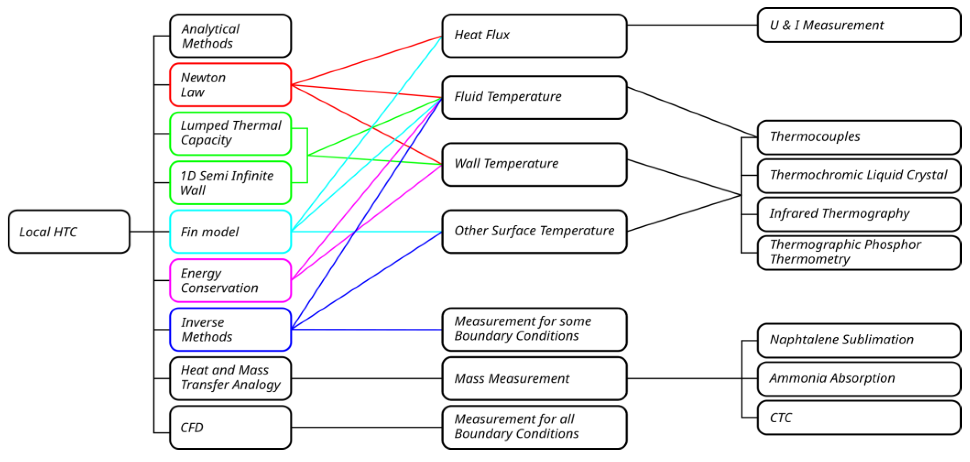
The most common method to determine the HTC is to use Newton’s law of cooling. For this purpose, all quantities, such as the heat flux, the fluid and the solid temperature, should be measured or calculated based on measured values. Other procedures can also be found in the open literature. They use analytical formulations, the lumped thermal capacity assumption, the 1D unsteady heat conduction equation for a semi-infinite wall, the fin model, energy conservation and the analogy between heat and mass transfer. The HTC distribution can also be calculated by means of computational fluid dynamics (CFD) modelling if all boundary conditions with fluid and solid properties are known.
Often, the surface on which the HTC is to be determined is not accessible for any measuring sensors, or their installation might disturb the analysed phenomenon. It also happens that calculations using direct or CFD methods cannot be performed due to the lack of required boundary conditions or sufficiently proven models to analyse the considered physical phenomena. Too long a calculation time needed by CFD tools may also be problematic if the method should be used in the online mode. One way to solve the above problem is to assume an unknown boundary condition and include additional information from the sensors located at a certain distance from the investigated surface. The problem defined in this way can be solved by inverse methods.
An overview of the methods currently used for the HTC determination is shown in Figure 1 and will be presented below.
2.1. Analytical Methods
Analytical solutions were developed for domains with a simple geometry, constant properties and uniform boundary conditions. For a laminar, hydrodynamically and thermally fully developed flow in a circular tube, which is heated by a uniform heat flux, Nu = 4.36. If the tube inner-surface temperature is constant, Nu = 3.66 [10]. An analytical solution for natural convection in a fluid-filled rectangular cavity was presented by Kimura and Bejan [11]. When the horizontal walls are adiabatic and the heat flux along the vertical walls is constant, Nu = 0.34 (H/L)1/9 Ra2/9, where H and L are the height and the length, respectively. Shahmardan et al. [12] developed an analytical solution for internal forced convection in rectangular channels assuming a fully developed laminar flow. Solutions were also presented for a constant heat flux at the boundary walls. Rybiński and Mikielewicz [13] presented an analytical solution for the Nusselt number in rectangular mini-channels for a fully developed laminar flow. The solution is in the form of a fast-convergent series, which is better than the double series proposed earlier. The idea of constant temperature at the duct circuit is associated with the typical condition in a mini-channel heat exchanger made of metal. Su and Freire [14] studied external forced convection over rod bundles with a smooth surface. They proposed the explicit equation for the Nusselt number associated with the turbulent flow. The same analytical method was applied to rod bundles with rough surfaces, but in that case, the Nusselt number was determined by numerical integration. D. Ghosh et al. [15] studied ferrofluid flows through parallel-plate ducts under a constant magnetic field. They assumed a hydrodynamically and thermally developed Couette–Poiseuille flow with three sets of thermal boundary conditions with different configurations of a constant temperature or a constant heat flux. The governing equations were simplified to generate closed-form solutions for Nusselt numbers as functions of the magnetic field strength, the nanoparticle volume fraction, the Brinkman number and the pressure gradient. The Brinkman number was defined as viscous dissipation heat per the wall heat flux. Poletto et al. [16] analysed the two-dimensional steady flow in a lid-driven square cavity exposed to a stable gravitational condition. They presented the equation for the area-averaged Nusselt number over the sliding-lid as a function of Gr, Re and Pr. These analytical solutions are presented for constant Nusselt numbers due to the adopted simplifications, or they are averaged in space.
Graetz [17] studied a fully developed laminar flow with a uniform temperature which flowed into the entrance with a uniform wall temperature. He assumed that the fluid axial conduction, the viscous dissipation flow work and the energy resources were negligible. The exact solution for the local Nusselt number as a function of the dimensional axial coordinate was presented. Minkowycz and Haji-Sheikh [18] presented the analytic series solution for a flow through parallel-plate and circular porous channels. The first part of the channel wall had temperature T1 and the second part, T2. The analysis included the contribution of axial conduction. The local Nusselt numbers were calculated from the exact solution and presented for selected Pe numbers. They were displayed as a function expressed as (x/H)/Pe or (r/RI)/Pe, where H is the distance between the plates and RI is the pipe inner radius, respectively. Weigand and Eisenschmidt [19] studied laminar or turbulent fully developed flows through a concentric annulus, exposed to constant temperature T1 at the first part of the outer wall and constant temperature T2 at the second part of the outer wall. The inner wall was adiabatic or kept at a constant temperature. They presented the analytical solution for the local Nusselt number as a function of the axial coordinate. Additionally, they proposed correlations that were obtained based on analytical solutions for selected radius-to-radius ratios χ = Ri/Ro and selected Pr and Re numbers. Zhao et al. [20] and Chen et al. [21] analysed heat transfer between horizontal surfaces and perpendicularly striking circular jets. Fourth-order polynomials were applied to approach the velocity and temperature profile. The analysis area was divided into the following four parts: the stagnation zone; the region with constant radial velocity equal to the jet velocity at the nozzle exit; the region where the viscous stress became appreciable, and the free-stream speed varied with r; and the region where both the flow and the thermal boundary layers were fully developed. The equations for the local Nusselt number were formulated in these four regions.
2.2. Newton’s Law
For a surface heated by a constant heat flux and cooled by a fluid, the HTC distribution can be determined from (1). Binark and Ozdemir [22] studied the effect of a pulsating airflow on the inner surface of a cylindrical duct with metal foam inside. The local HTC was calculated using Equation (1). To measure the surface temperature, 30 K-type thermocouples were installed in holes with a diameter of 1 mm and a depth of 4 mm. Thermal paste was used to fill the holes to ensure good thermal contact between the sensors and the duct. The temperature of the air was measured using copper-sheathed thermocouples placed in the duct centre. A constant heat flux was applied using an electric heater. The surface heat flux was obtained by measuring the electric power of the heaters and taking into account thermal losses through 15 mm glass wool insulation. Unfortunately, the method of the surface temperature measurement caused uncertainty limits similar to the temperature difference between the steady and the pulsating flow.
Piasecka et al. [23] studied subcooled boiling heat transfer during a flow in a mini-channel heat sink with three or five 1 mm deep mini-channels. The heated thin foil, made of the Haynes-230 alloy, was cooled using the Fluorinert FC-72 fluid. An infrared camera was used to measure the foil temperature distribution. The inlet and outlet temperatures were measured by K-type thermocouples. The local HTC was determined using Newton’s law. The local fluid temperature Tf was calculated as linear dependence between the inlet and the outlet temperature of the mini-channel. The heat flux was determined based on the measured electric power supplied to the heater. The variation in the heat flux along the flow was ignored in this approach. Additionally, the finite element method with the Tretz-type basis functions was applied to take into account the two-dimensional heat transfer in the foil. The relative difference between the 1D and the 2D approach for the average HTC on the foil surface was about 12.8%. The average uncertainties of the HTC determination in the subcooled boiling region using the 2D approach were estimated at about 20%.
2.3. Solution for a Body with Lumped Thermal Capacity
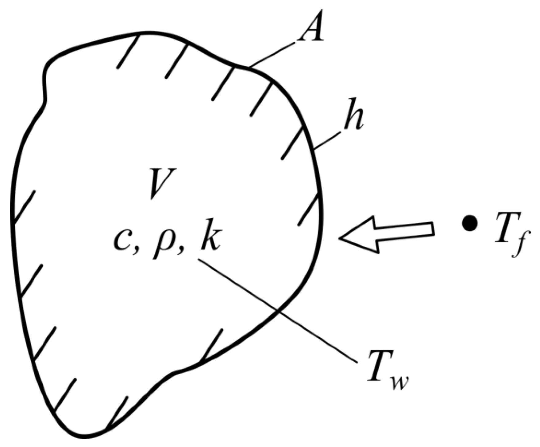
Lykov and Smol’skii [24] proposed a method of determining the transient heat transfer coefficient on the outer surface of metal balls. For thin-walled balls with high thermal conductivity, the heat transferred from the fluid is completely utilized, increasing the ball internal energy. The Biot number is less than 1, and the model with lumped thermal capacity can be used to calculate the HTC:
where A is the ball outer surface area [m2], V is the ball volume [m3], T0 is the initial temperature, Tf is the fluid temperature (°C) and Tw is the measured body temperature (cf. Figure 2). The material properties c—specific heat and ρ—density should be known. This method can be applied if the heat transfer from the fluid to the solid is completely utilized, increasing the internal energy of the solid (Bi < 1).
Abuaf et al. [25] used the same method in a warm-wind-tunnel test facility equipped with a linear cascade of film-cooled vane aerofoils for the HTC estimation. The surface temperature was measured using the thermochromic liquid crystal (TLC) technique. Compared to the single-point measurement by thermocouples, the TLC method is contactless and highly precise. It provides a complete temperature distribution and does not destroy the flow field. However, its application is limited to temperatures lower than 200 °C and requires precise control of lighting conditions. The application of this measurement technique for the HTC estimation was described by Stasiek [26].
Mikheev et al. [27] obtained the local HTC distribution over a cylinder surface depending on the flow pattern. A cylinder with a wall thickness of 2 mm was made of polypropylene. Type-L thermocouples were mounted in the cylinder wall close to the outer surface. After they were installed, the surface of the cylinder was processed to bring it back to its initial smooth state. Due to the small thickness of the cylinder wall, the model with lumped thermal capacity was also used to determine the HTC. The Biot number calculated on the basis of the wall thickness was less than 0.1. The heat transfer coefficient on the cylinder outer surface was calculated from Equation (2), where SA is the area of the heat-release surface of the cylinder [m2], WV is the cylinder wall volume [m3], T0 is the initial temperature of the cylinder wall, Tf is the fluid temperature (°C) and Tw is the temperature measured on the cylinder outer surface.
Buchlin [28] studied the convective heat transfer between impinging gas jets and a heated thin plate. He applied infrared thermography (IR) to scan the rear face of the plate while the jets were directed at the front part. The rear face was coated with black paint to improve the measurements. The Biot number was small enough (<0.1) to ignore temperature variation through the plate thickness. The local convective HTC was therefore calculated from Equation (1).
2.4. Solution of 1D Unsteady Heat Conduction in a Semi-Infinite Wall
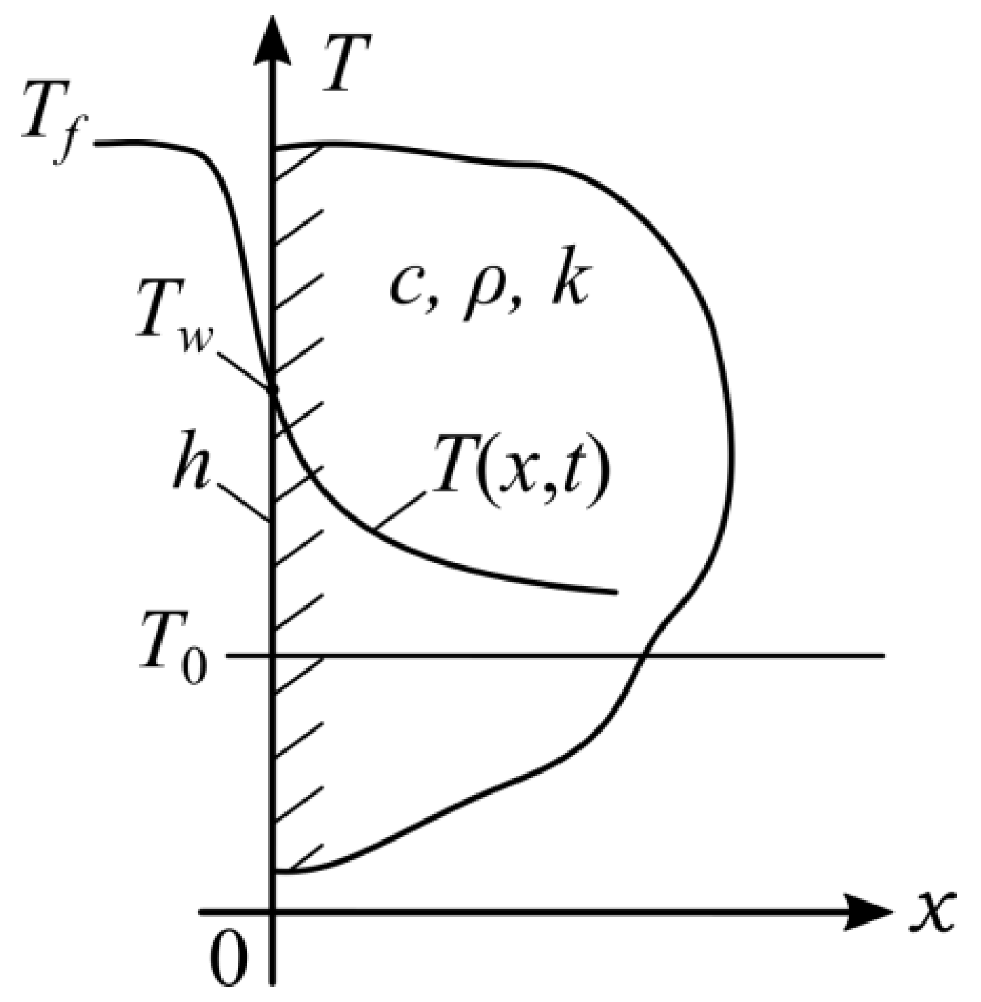
Facchini et al. [29] presented an experimental study of heat transfer in ribbed channels in the turbine blade cooling system at the entrance region. Thermochromic liquid crystals were sprayed on one surface of the channel. The turbine blade was made of a material characterized by low thermal diffusivity and was thick enough to be analysed as a semi-infinite block with a one-dimensional temperature distribution. The normal surface temperature response of the poly methyl methacrylate channel under a step change in the fluid temperature was calculated using the analytical solution of 1D transient heat conduction in a semi-infinite wall, as presented in Figure 3. The solution described by Carslaw and Jaeger [30] has the following form:
where erfc() is the complementary error function. The local HTC on the test surface can be obtained from Equation (3). A similar method was used by Chen et al. [2] to calculate the two-dimensional HTC on a flat jet plate and by Kong et al. [3] on a corrugated jet plate.
In real conditions, it is difficult to obtain a jump in the fluid temperature from T0 to Tf. For this reason, the fluid temperature Tf is divided into small steps, and the Duhamel superposition rule is used, as presented by Taler and Duda [31].
where Tf,i is the fluid temperature measured at time ti, and N is the number of time steps. The local HTC on the test surface was calculated using Equation (4).
Bizzak and Chyu [32] tested a novel thermal imaging system for local convective heat transfer analysis. One surface of a quartz disc was coated with a 25 μm layer of thermographic phosphor La202S: Eu3+. The experiment consisted in directing a stream of air from an impinging heated jet onto the quartz disc. The HTC was calculated assuming that initially, the isothermal disc subjected to heating by a constant-temperature jet behaved like a semi-infinite body. The unsteady process should be short enough to avoid heat transfer to the back surface of the test piece. For this reason, the time of a single measurement had to be limited to 30 s. The estimated HTC uncertainty was 11%.
Yi et al. [33] used thermographic phosphor thermometry to determine the HTC distribution on a hot plate cooled by an oblique jet. The test surface was coated with thermographic phosphor and treated as a one-dimensional semi-infinite solid model. The HTC distribution was obtained from Equation (3) or (4). The accuracy of the method depended on the correctness of the temperature measured by means of thermographic phosphor thermometry. Manganese-activated magnesium fluorogermanate was used because it has continuous decay characteristics of phosphorescence and can be applied in higher temperatures. The decay-slope procedure was applied for calibration, and the temperature measurement uncertainty was ±3% for the temperature range of 130–530 °C. This method has a much wider range of applicability than TLC or IR. Mg4FGeO6:Mn can cover a wide range of temperatures from 13 K to more than 1000 K. The calculated HTC distribution in time and space was presented. The maximum HTC appeared at the stagnation point and decreased gradually in time.
2.5. Fin Model
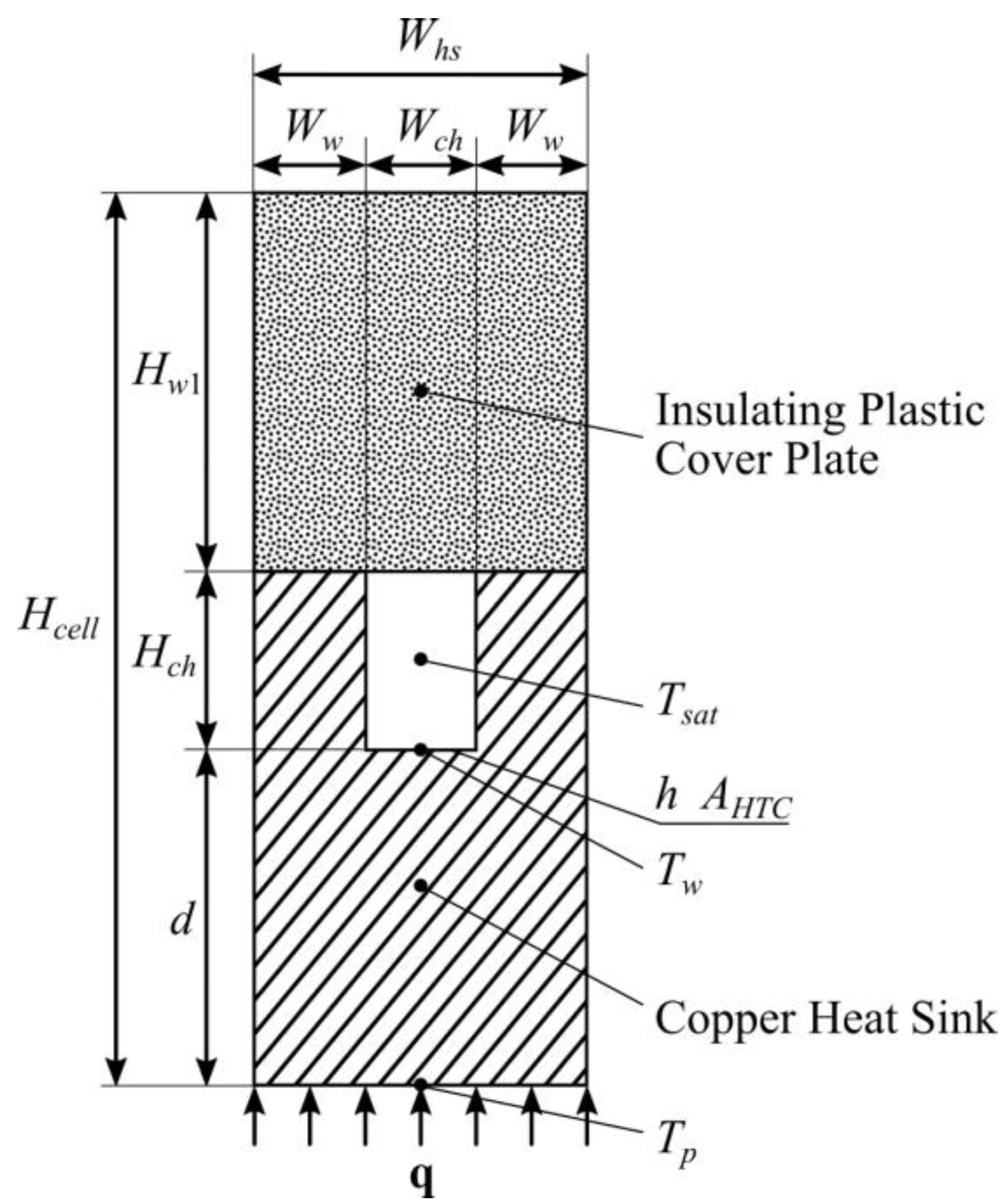
Qu and Mudawar [34] predicted a saturated flow boiling heat transfer on the surface of a water-cooled micro-channel for both single- and two-phase flows. The test module contains twenty-one parallel micro-channels with a hydraulic diameter of 341 μm. Cartridge heaters were installed to heat the underside of the copper block and their power was measured. Type-K thermocouples and pressure transducers measured the fluid parameters at the channel inlet and outlet. Additionally, four type-K thermocouples were located along the flow direction at a certain distance from the surface to determine the channel bottom-wall temperatures. After setting the parameters of the flow loop components, the heatsink was allowed to reach a steady state in each test. It was assumed that the heat flowed mainly in the direction normal to surface AHTC, on which the HTC was determined. The proposed method is based on measurements of the fluid local temperature, the micro-channel wall temperature at a distance from AHTC and the heat flux.
Through the fin analysis applied to the unit cell, which is shown in Figure 4, the following energy balance equation is formulated:
where Tw is the channel bottom-wall temperature, which can be calculated using temperature Tp measured at distance d from surface AHTC.
Tsat is the water saturation temperature at the thermocouple location, Wch is the micro-channel width, Hch is the micro-channel height, Whs is the width of the heat sink unit cell, η is the fin efficiency, k is the copper heat sink thermal conductivity and q is a constant heat flux calculated using input electricity supplied to the heaters. It should be emphasized that h cannot be determined explicitly from Equation (5) because the fin efficiency η is a function of h.
Lee and Mudawar [35] applied the same technique to determine the HTC in a micro-channel cooled by water-based nanofluids containing small concentrations of Al2O3. Both single-phase and two-phase flows were analysed. This approach is valid in regions where heat conduction can be approximated as one-dimensional.
2.6. Heat and Mass Transfer Analogy
Kang and Lee [36] analysed the geometric dimensions of the turbine blade in terms of heat and mass transfer rates. The naphthalene sublimation approach was used to obtain the distribution of Sherwood and Nusselt numbers on the outer surface of the turbine blade. This method makes use of the analogy between heat and mass transfer and was described in detail by Goldstein and Cho [37]. A mould for casting naphthalene was made in the shape of a turbine blade. The prepared model was placed in a cascade wind tunnel. The sublimation depth was measured at 630 points using an ultra-precise depth gauge. The mass transfer coefficient hm was determined from the local sublimation depth. The HTC distribution can be calculated from the Nusselt number (Nu), which is a function of the Sherwood number (Sh):
where Pr is the Prandtl number, Sc is the Schmidt number and coefficient n is 1/3 for a laminar flow and 0.4 for a turbulent flow. The uncertainty of Sh calculated with 95% confidence was estimated at ±6.4%.
Ahrend et al. [38] employed the ammonia absorption method to determine the local HTC distribution on two heat exchangers. The determined HTC distributions made it possible to choose a better solution in terms of heat transfer.
Che and Elbel [39] proposed a new method to determine the local air-side HTC based on the analogy between heat and mass transfer. An aluminium plate was coated with AMS 67 instead of naphthalene. The used plate mean roughness was 0.9 μm, and after applying the spray, 1.6 μm. Mean coating thicknesses ranged between 5.8 and 5.5 μm. The thickness was thus significantly smaller than the thickness of the applied naphthalene layer, which can be as much as 200 μm [37]. A coated specimen was located in the wind tunnel below a transparent polycarbonate sheet to be seen by the installed camera. The coating material absorbed tracer gas and changed its colour during the experiment. Based on the performed visualization procedure, the observed colour was correlated with the local mass transfer coefficient. Finally, the local HTC was calculated from the following equation:
where Mmax is the maximum mass of ammonia gas absorption [kg], ΔC is the concentration difference [kg/m3], A is the total surface area of the specimen [m2], ε is a coefficient calculated through image processing [-] and S is the colour change factor [-] obtained during the calibration procedure. Thermal conductivity k [W/mK] and diffusion coefficient D [m2/s] of ammonia in air are known properties. The measured local HTC for the air velocity in the range of 0.6 to 3.0 m/s agreed with the Blasius solution on the flat plate. The uncertainty of the measured local HTC on the flat plate in the laminar flow was estimated at 15%. Another advantage of this method is that the coated surfaces are stable for at least 45 days. The method was named by the author as the acronym of coating tracer colour—CTC.
2.7. Energy Conservation
Heinze [40] proposed a consistent mathematical model for the calculation of the HTC in deep underground geothermal systems. The heat transfer between rock and fluid is described by Newton’s law of cooling (1), which can be transformed into the following form:
where Q [W] is the heat rate, A [m2] is the heat convection area and Tf and Tr are fluid and rock temperatures, respectively. Determining the HTC from this equation is difficult, so Heinze developed a method based on the heat balance between fluid and rock. He assumed that the heat absorbed by water in the whole pathway of the fracture was equal to the convective heat transfer between water and the inner surface of the fracture on the basis of energy conservation. The transient heat balance equation for fluid at any point x along the fracture surface has the following form:
where cf is the water specific heat capacity, ρf is the water density, u is the water velocity and is a source term generated by the heat transfer between both phases. It can be calculated as heat transfer per the fluid volume in the fracture:
where e is the fracture aperture, as can be seen in Figure 5. Equation (11) in the steady state takes the following form:
where the fluid volume and the heat convection area equal, respectively, . Integration of this equation and the use of the two boundary conditions presented in Figure 5,
make it possible to express the HTC as
Additionally, Heinze showed how to compute the lower bound of the HTC between rock and the flowing medium in a single rock fracture. This is useful in geothermal reservoir feasibility studies as the worst-case scenario. He also presented approximations for the upper limit of the HTC using the results of experimental studies available in the literature.
He et al. [41] studied heat transfer in the case of water flowing through a single granite fracture. The analysis of this phenomenon is applicable in deep underground geothermal systems. The HTC was calculated from the following equation:
where Tx1 and Tx2 are the temperatures of two points close to the inner surface of the fracture along the flow direction, and x1, x2 are x coordinates of these points. A number of heat transfer experiments using cylindrical granite specimens were conducted for different pressures and flow rates. The flow was proven to be laminar. The local HTC distribution along the flow direction was completely different from the average HTC. The variation in surface roughness had a big effect on the local HTC distribution, while the aperture and the flow rate had no major impact.
2.8. CFD
Xing et al. [42] presented a numerical study of the cooling of a turbine blade leading edge using air. The determined HTC distributions show the influence of the surface curvature, the distance of the jet from the surface and the cross-flow type on cooling performance. Considering the single-phase nature of the flow, classical methods of continuum mechanics are used to solve the mass, momentum and energy conservation equations. Additionally, the improved two-equation K-Omega turbulence model [43] is used. All boundary conditions needed to solve the above equations must be presented for the fluid and solid regions. The air velocity and turbulence intensity are defined at the impingement and cross-flow inlets. Static pressure was defined at the outlets. No-slip boundary conditions are specified on all walls of the computational domain. The cross-flow inlet, the impinging jet and the target surface temperatures are also specified. The advantage of the numerical approach is the ability to run a large number of tests. Selected cases were verified using the experimental results obtained by Funazaki et al. [44].
Abdelfattah et al. [45] applied numerical modelling for a staggered semi-circular tube bank to evaluate its thermal and hydraulic characteristics. Using the determined HTC distribution, places with the best and the worst heat exchange were located. For all tubes, the maximum local HTC occurs around the upstream corner, where the flow initially stagnates. The minimum value is observed around the separation point. The calculations were carried out for an incompressible fluid with constant physical properties. The four-equation SST model [46] was applied for turbulence analysis. The calculation area was enlarged so that the inlet and outlet were located at a distance of 25 tube diameters from the bank. In this way, the boundary effects were minimized. All boundary conditions related to turbulence intensity, inlet velocities, outlet pressures and no slipping on walls were defined. Additionally, constant air inlet and tube surface temperatures were specified. Only average Nu values were compared to experimental results. The highest relative error between numerical and experimental data by Zukauskas [47] is 0.46%.
Peng et al. [48] investigated the coupled transcritical–condensation flow in a printed-circuit heat exchanger. A numerical model of a double-bank semi-circular straight channel is used to calculate the local HTC on both the hot and the cold side. The presented HTC distributions for the side of the condensation flow and the transcritical flow explain why the area of the heat transfer drop occurs in the transcritical flow. The cause is the large heat flux concentration, whereas the HTC weakening disappears immediately when the condensation process is completed. To reduce the calculation cost, one double-bank channel unit was modelled instead of the entire heat exchanger by introducing periodic boundary conditions. Additionally, mass flux inlet and pressure outlet boundary conditions are specified for hot and cold fluid. A constant heat flux was defined between hot and cold fluid. The volume-of-fluid (VOF) method [49] was used to analyse the multi-phase flow, and the interface between liquid and vapour was formed as a result. The shear stress transport k-ω turbulence model [50] was applied. The HTC of the transcritical heating process was compared to the experimental data published by Li et al. [51]. Satisfactory agreement was obtained only in the near pseudo-critical region.
Chen et al. [52] studied three-dimensional heat transfer during falling film evaporation in a horizontal tube using computational fluid dynamics. The HTC distribution was investigated for the droplet flow, the column flow and the sheet flow through the tube. For all the cases under analysis, a three-dimensional distribution of the HTC was obtained. The smallest changes appeared in the longitudinal direction for the sheet flow regime. The largest changes occurred in the circumferential direction for all the cases. Noteworthy are the changes in the determined values. When the tube wall temperature varied, for example, between 333.4 K and 336.9 K, the change in the HTC was between 0 and 45 kW/m2 K. The determined HTC distributions describe the analysed phenomenon more clearly. The presented numerical model included two halves of the tube due to the applied symmetry condition. The top tube has an adiabatic boundary condition and the bottom one is heated with a constant heat flux. This resulted in a uniform falling film around the top tube and the appropriate flow pattern between the tubes and the bottom tube. Calculations were made for the incompressible flow and a laminar film. The VOF method [49] was applied to analyse the interface between liquid and vapour using a continuity equation. The continuum surface force model elaborated by Brackbill et al. [53] was utilized to compute surface tension. The second-order upwind scheme was applied in the momentum and energy equation discretization. Equation (1) was used to calculate the HTC, where TF is the saturation temperature instead of the fluid temperature.
Soleimani et al. [54] simulated a micro-channel heat sink cooled by two-phase flow boiling. Such a micro-channel heat sink was previously experimentally tested by Lee and Mudawar [35]. The calculated local HTC decreased along the micro-channel length in the single-phase flow zone because the thermal boundary layer increased. After the onset of nucleate boiling, as a result of the disturbance to the thermal boundary layer caused by the movement of bubbles, the local HTC started to grow. The calculated local HTC changes led the authors to the conclusion that remarkable heat transfer enhancement could be obtained due to the use of nanofluid mainly for two-phase flows and not for single-phase flows. The obtained numerical results were compared with experimental results [35]. The maximum error in the HTC calculation is below 6%.
Kang et al. [55] proposed a reduced-order model based on a machine-learning approach and proper orthogonal decomposition (POD) to reduce the calculation time of the Navier–Stokes equations in the CFD method. They applied the proposed method to reconstruct the rod bundle flow field. The calculations were carried out in two and three dimensions. The benefits of the proposed method appear when the calculations are carried out within the range of training parameters. A significant reduction in the calculation time was obtained, keeping appropriate accuracy of the calculation.
Wang et al. [56] studied the application of POD to solve complex heat transfer problems. They compared POD interpolation and POD projection procedures. The POD projection method is faster and more accurate in the analysis of complex thermal-flow problems.
2.9. Inverse Methods
Freund et al. [57] proposed temperature oscillation IR thermography to measure the spatial distribution of the HTC. A spray cooling system was installed under a steel sheet, while a laser and an IR camera were positioned above the sheet top surface. The HTC distribution on the bottom surface of the plate was determined despite the lack of information about the fluid temperature and properties. The measured heat flux which was sent by the laser onto the steel sheet upper surface and the temperature distribution recorded by the IR camera were used. The inverse heat conduction problem of deriving the HTC distribution from the phase-lag data was solved despite the unknown boundary condition on the bottom surface of the plate. For this purpose, a complex 3D finite-difference method was used. The identified HTC distributions showed significant maldistribution of the heat transfer efficiency.
Freund and Kabelac [58] applied the same method to a plate heat exchanger. The identified local HTC in some areas was about two to three times higher than the average HTC value. In addition, CFD modelling was carried out using several turbulence models. Noteworthy is the uncertainty analysis carried out for the experimental and numerical methods. The uncertainty of the arithmetically measured area-averaged HTC was about 12%. In numerical calculations, depending on the turbulence model, 33% was for the SST and 25% for the RSM–EASM approach.
Divo et al. [59] developed an inverse BEM-based regularized algorithm to calculate the HTC distribution from transient surface temperature measurements. A regularized functional was minimized to approximate the recent heat flux. This procedure also made it possible to smooth out uncertainties of calculated HTC values due to experimental errors in measured temperatures, which is significant in the stabilization of an ill-conditioned inverse solution. Due to the use of the BEM method, only the edge of the area was discretized, and therefore, the temperature measurement points are on this edge. Despite measuring the temperature on the surface where the HTC is identified, the algorithm requires stabilization. The regularization parameter controlled the solution smoothing, suppressing large deviations from measured temperatures. The performed numerical tests showed the stability and accuracy of the method. The method was applied to a simple area only and the physical properties were assumed to be independent of temperature. In addition, the method was tested experimentally. Air was heated to 60 °C and directed over an aluminium block which simulated a plane turbine blade tip surface. At the beginning of the experiment, the block was heated to a steady-state temperature of 51 °C. A 0.1–0.2 mm thick TLC coating was applied on two surfaces of the block. The TCL coating made it possible to measure temperatures in the range of 35 to 55 °C. The identified HTC was relatively constant in time but varied significantly in space. A big change in the HTC occurred around the rounded corner. This effect would not be captured by models based on lumped heat capacity or one-dimensional heat conduction.
Bozzoli et al. [60] proposed the inverse method to identify the local convective HTC at the fluid wall interface in coiled tubes based on the temperature measured on the external coil and bulk temperature. The distance of the inlet section from the measuring section was large enough to obtain a laminar flow inside the tube. One coiled tube section was not insulated, and its outer-surface temperature was measured using an infrared camera. The surface was locally not normal to the viewed rays, but the viewing angle was limited to ±30°, and it was assumed that the surface behaved as a diffuse grey emitter. The effective emissivity of the outer-surface coating was estimated by a number of tests at different known temperatures, and the value of 0.99 was determined. In addition, ambient temperature and the HTC on the outer surface were assumed. The bulk temperature at any location in the heat transfer section was computed taking into account the power supplied to the tube, the heat losses through the insulation, and the inlet and outlet fluid temperature. Additionally, the wall thermal conductivity was equal to 15 W/m K, and the heat generated by the Joule effect in the wall was computed by relating the supplied power to the tube wall volume. In the inverse algorithm, the calculated temperature field is forced to match the experimental temperature distribution by selecting the convective heat flux distribution on the internal wall side. The problem is ill posed and the Tikhonov regularization method is used to stabilize the solution. Numerical tests made it possible to select the optimal value of the regularization parameter of 1.17 10−5. Finally, the HTC was calculated from Equation (1) for each point on the inner surface. The calculated local HTC along the measuring section indicated that its minimum value occurred close to the inner-bend side of the coil. It reached the maximum value at the outer-bend side due to the onset of secondary flows induced by the wall curvature. The uncertainty analysis showed that the main contributions to the HTC uncertainty were the tube thermal conductivity and the heat generation rate measurements. The uncertainties of the outer-surface HTC and ambient temperature measurements are almost insignificant.
Bozzoli et al. [61] applied the same method to estimate the local HTC distribution on the inner surface of coiled tubes for a turbulent flow regime. Like for the previously analysed laminar flow, the local HTC minimum value occurred at the inner-bend side, while the maximum value was at the outer-bend side of the coil. The differences between them are greater than in the laminar flow. The HTC at the outer surface is approximately ten times larger than at the inside surface, and this ratio is almost independent of the Reynolds number. The sensitivity analysis indicated that the main contributions to the uncertainty were the tube thermal conductivity, the heat generation rate and the bulk temperature measurements, while the uncertainties of the outer-surface HTC and the ambient temperature measurements are not very significant.
Cattani et al. [62] proposed the inverse procedure to identify the local convective HTC for thin-liquid-film evaporation in a capillary tube. The method, previously developed for steady states, was extended for transient analysis. The measurement of the temperature distribution over time enabled analysis of the vaporization process in a capillary copper tube. The accuracy and stability of the method were first demonstrated in a numerical test. The HTC was assumed in the form of a step function that varied both in time and space. The direct solution made it possible to generate a temperature field on the tube outer surface. The temperature transients that were needed for the inverse method were distorted by random errors. The numerical verification showed the effectiveness of the presented algorithm at various noise levels. Finally, the inverse method was applied to estimate the HTC distribution for a semi-infinite slug flow in a tube with uniform heat generation in its wall due to the Joule effect. The outer-surface temperature of a capillary tube was measured by an infrared camera. The tube wall thermal conductivity was equal to 401 W/m K, and the generated heat was calculated by relating the supplied power to the tube wall volume. The surrounding air temperature and the HTC on the outer-tube surface were estimated. The fluid bulk temperature was assumed to be equal to the saturation temperature measured in the tank from which the fluid flowed. Based on the estimated HTC distribution over time, four different time zones were established. They were characterized by different heat transfers in the tube when the meniscus that separates the liquid phase from the gas phase was intersected. In the first zone, convective heat exchange occurred as a result of the laminar flow in the tube. In the second, a meniscus transition took place, during which thin-film evaporation occurred. In this area, very high values of the HTC were registered. They remained at a similar level in the third zone, where thin-film evaporation was detected. The last zone illustrated a linear reduction in the HTC caused by an increase in dry spots on the channel wall. The uncertainty of the identified HTC was estimated based on numerical tests and totalled about 13%.
Mobtil et al. [63] studied the transient HTC distribution over the fin of a staggered finned-tube heat exchanger assembly. The circular fin was located in a small wind tunnel with an IR transparent window mounted on top of the test section. In the first part of the experiment, there was no airflow through the test section, and an infrared-emitting heater heated up the fin through the IR transparent window. During the second part, the cooling period, the infrared heater was replaced with an IR camera which recorded the temperature distribution on the fin upper surface. It was assumed that the fin was thermally thin, so temperature changes through the fin thickness were omitted. The measured inlet air temperature was taken as the bulk temperature. To determine the local HTC distribution, it was still necessary to calculate the heat flux field on the upper surface of the fin. For this purpose, an iterative inverse algorithm was proposed. It was formulated as a nonlinear optimization problem with an iterative gradient-based method. Temperature-independent material properties were used. The iteration process was stopped when the differences between the estimated and measured temperatures were close to the temperature measurement errors. The identified local HTC values were high near the leading edge of the fin, upstream of and around the tube. Low values were estimated downstream of the tube and were caused by low velocity in this area. Twelve K-type thermocouples were installed on the outer surface and eight at different points along the thickness of the collector wall.
Duda and Konieczny [64] analysed the HTC distribution in time and space on the inner surface of a horizontal thick-walled collector, which was divided in half using a horizontal 5 mm thick partition. The collector with the initial temperature of 22 °C was heated by the flow of oil with the temperature of 180 °C through its lower part. The air temperature in the laboratory hall, the HTC and the emissivity value on the collector outer surface were determined. Additionally, the temperature and pressure of the flowing oil were measured during the collector heating process. The inverse transient heat conduction problem was solved using the proposed space-marching method, and the HTC distribution in time and space was calculated based on the measured values. To improve the solution stability, smoothing digital filters were used. The phenomena occurring inside the collector were identified. Despite the sealing, full tightness was not achieved. The HTC showed that the flow of hot oil occurred mainly near the right end of the partition. The accuracy of the inverse method was assessed by comparing the calculated and measured temperature transients at points inside the collector wall that were not used during the identification.
Duda and Konieczny [65] presented a new algorithm to identify the temperature and the HTC distribution in any extended complex domain. The inverse transient heat conduction problem was solved based on temperature transients which were generated on the easily accessible outer surface. The control volume finite element method was applied to solve problems that occur in elements with complex geometries and temperature-dependent material properties. The solution was stabilized by smoothing digital filters and by dividing the space domain into several subdomains with free boundary conditions between them. The HTC values estimated on the component inner surface after 100 s and 200 s of the heating operation were presented. This means that inverse methods can be used to determine the unsteady HTC distribution on the inner surface of an element, despite the fact that it is impossible to install sensors on the element surface. The methods can be applied in practice, for example, in a nuclear power plant, where it is impossible to drill holes to install measuring sensors.
3. Local Heat Transfer Coefficient Correlations
Analytical, numerical and experimental studies made it possible to develop correlations for local Nusselt numbers. The first correlations were given for steady, incompressible laminar flows in a pipe. Natural convection, phase change processes, mass transfer or chemical reactions were not taken into account. Work and energy dissipation in a viscous flow were also omitted. A Newtonian fluid with a fully developed velocity distribution and a uniform temperature flowed into the entrance with a uniform wall temperature. Shah and London [66] proposed the correlations for the local Nusselt number as the function of dimensionless coordinate x*:
where
The presented correlations can be used for the simplifying assumptions given above and for a thermally developing flow with .
The dimensionless thermal entrance length can be calculated from the following equation:
If the flux density on the channel walls is constant, instead of a constant temperature, the equations take the following form:
The correlations for the local Nusselt number versus a dimensionless coordinate were also given for a hydrodynamically and thermally developing laminar flow between plates [66].
Theoretical and experimental studies of the heat transfer from horizontal surfaces to normally impinging circular free-surface jets made it possible for Zhao et al. [20] to propose a correlation for the local Nusselt number as a function of the distance from the stagnation point ζ. The measurements were carried out under steady-state conditions. At the outlet of the nozzle, which was positioned vertically above the plate surface, the water had a fully developed velocity distribution. Measurements were carried out and correlations were developed in the range of Re numbers from 5000 to 24,000. The ratio of the distance between the nozzle and the plate to the diameter of the nozzle varied from 2 to 10. The correlations which are presented in Table 1 below enable determination of the local Nusselt number for distances from the stagnation point not greater than eight nozzle diameters.
4. Summary and Conclusions
The non-uniform HTC distribution is often significant in the design and operation of devices and in explaining the physical phenomena occurring in them. Despite many studies on the HTC determination, it is not possible to indicate the best method. Most of the available analytical solutions are presented for constant Nusselt numbers due to the applied simplifications, or they are averaged in space. If the heat flow is mainly normal to the surface on which the HTC is measured, Newton’s law with the measured heat flux generation can be applied directly. If the heat also flows in other directions, this procedure may lead to errors. The relative difference between 1D and 2D approaches for the average HTC on the foil surface can be about 12.8% [23]. If the heat transferred from a fluid is completely utilized to increase the internal energy of the element on which the surface HTC should be determined, the model with lumped thermal capacity can be used. This is the case if the Biot number calculated based on the wall thickness is lower than 0.1. The method can be used when the heat flux is unknown. If the heating or cooling of the body proceeds in such a way that the temperature changes only near the surface, the solution of the one-dimensional heat conduction equation in a semi-infinite wall can be used. The duration of a single measurement process should be short enough to avoid heat penetration to the back surface of the tested specimen. Various methods can be used to measure the surface temperature. The use of thermocouples does not require a calibration process. The TCL method is contactless and highly precise. It provides a complete temperature distribution and does not destroy the flow field. However, its application is limited to a temperature of about 200 °C. The IR procedure can be applied to higher temperatures, but its accuracy is limited by the influence of surface materials and temperature changes on its emissivity. Thermographic phosphor thermometry can be applied to temperatures between 13 K and 1000 K. The temperature measurement uncertainty reported in 2016 totals about ±3% for the temperature range of 130–530 °C [33]. In recent years, significant progress has been made in terms of the range and accuracy of the temperature field measurement. If for some reason it is not possible to measure the temperature on the surface on which the HTC should be determined, and if it is possible to assume heat conduction in the direction normal to the surface, then the fin model can be applied. For simple and complex geometries with multidimensional heat conduction, the analogy between heat and mass transfer can be used. The HTC can be determined based on the measured sublimation depth of the naphthalene coating. Other materials, such as AMS 67, can now be used instead of naphthalene. The coating material absorbs tracer gas and changes its colour during the experiment. Based on the performed visualization procedure, the observed colour is correlated with the local mass transfer coefficient and finally the local HTC can be determined. The thickness of the coating is much smaller, the durability of the coating is longer and the accuracy of the determined HTC is higher compared to tests using naphthalene. In the case of the phenomena for which it is difficult to determine the exact location of the surface where the HTC should be determined, it is more convenient to use the energy conservation equation. A good example is the determination of the local HTC between rock and flowing fluid in a single rock fracture. This method can also be used for multiphase flows. A commonly used method to determine the local HTC distribution is CFD. All boundary conditions with fluid and solid properties should be known. For single-phase laminar flows, classical methods of continuum mechanics are used to solve the mass, momentum and energy conservation equations. For turbulent or multiphase flows, additional models are required, the proper selection of which is crucial for the determined HTC distributions. The adopted discretization of the computing area is also of great importance. With properly selected settings of the CFD model, it is possible to obtain accuracy even below 6% compared to experimental results [35], but the differences between the results obtained from different turbulence models can be at the level of 8% [58]. Often, the surface on which the HTC needs to be determined is not accessible for any measuring sensors, or their installation might disturb the analysed phenomenon. If the fin model cannot be applied because heat conduction in a solid is not one-dimensional, the inverse problem can be formulated. It is assumed that the surface on which the HTC should be determined has an unknown boundary condition. To solve the problem, additional information is introduced, usually related to the measured temperatures. The problem defined in this way is ill conditioned. Various methods of stabilizing the inverse algorithm are used, such as the Tikhonov regularization, the application of smoothing digital filters or the division of the space domain into several subdomains. Based on the literature review, the following directions for further work can be indicated.
- Future works should concern a further improvement in measurement methods that can be used for HTC determination. It is necessary to conduct a comparative study between different procedures to compare them qualitatively and quantitatively. It would be valuable to show the range of applicability of selected techniques and consistent estimates of their accuracy.
- The possibility of using selected techniques on an industrial scale should be taken into account. At this point, the need for inverse algorithms arises, because the surfaces where the HTC is to be determined are often inaccessible for measuring sensors. In this case, the HTC uncertainty depends not only on the measurement uncertainties but also on the applied inverse algorithm.
- Effective methods should be developed to calculate the unsteady HTC distribution on surfaces where it is not possible to place any sensors and for objects with a complex shape.
- Further research on exact solutions and on correlations for Nusselt numbers as a function of the spatial position is recommended.
Funding
This research received no external funding.
Data Availability Statement
Not applicable.
Conflicts of Interest
The author declares no conflict of interest.
Nomenclature
| a | Thermal diffusivity [m2/s] |
| A | Surface area [m2] |
| c | Specific heat [J/(kgK)] |
| C | Concentration [kg/m3] |
| d | Distance, diameter of the cylindrical rock specimen [m] |
| D | Mass diffusivity [m2/s] |
| Dh | Hydraulic diameter [m] |
| e | Fracture aperture [m] |
| h | Heat transfer coefficient [W/(m2K)] |
| H | Channel height, rock height [m] |
| k | Thermal conductivity [W/(m K)] |
| L | Channel length, rock length [m] |
| M | Mass [kg] |
| Nu = hδ/k | Nusselt number [-] |
| Pe = RePr | Peclet number [-] |
| Pr = ν/a | Prandtl number [-] |
| Q | Heat flux [W/m2] |
| Q | Heat rate [W] |
| QV | Source term per unit volume [W/m3] |
| P | Wetted perimeter of the cross-section [m] |
| R | Radius [m] |
| R | Radius [m] |
| Ra = Gr Pr | Rayleigh number [-] |
| Re = uδ/ν | Reynolds number [-] |
| S | Colour change factor [-] |
| Sc = ν/D | Schmidt number [-] |
| Sh = hδ/D | Sherwood number [-] |
| T | Time [s] |
| T | Temperature [°C] |
| u | Velocity [m/s] |
| V | Volume [m3] |
| W | Width [m] |
| We = ρuδ/σ | Weber number [-] |
| x | x coordinate [m] |
| Greek symbols | |
| δ | Characteristic length [m] |
| ε | Coefficient from image processing [m] |
| η | Fin efficiency [-] |
| ν | Kinematic viscosity [m2/s] |
| Ρ | Density [kg/m3] |
| χ = Ri/Ro | Inner-to-outer radius ratio [-] |
| Ζ | Radial distance from the stagnation point [m] |
| ζn | Nozzle diameter [m] |
| ζ0 | Radius at which ∆reaches liquid film thickness [m] |
| Σ | Surface tension of the water [N/m] |
| ∆ | Hydrodynamic boundary layer thickness [m] |
| Subscripts | |
| c | Cross-section |
| ch | Microchannel |
| hs | Heat sink |
| I | Inner |
| max | Maximum |
| P | Measurement point |
| R | Rock |
| f | Fluid |
| w | Wall |
| 0 | Initial |
| O | Outer |
| Abbreviations | |
| BEM | Boundary element method |
| CFD | Computational fluid dynamics |
| CTC | Coating-tracer-colour method |
| HTC | Heat transfer coefficient |
| IR | Infrared thermography |
| TLC | Thermochromic liquid crystal |
| VOF | The volume-of-fluid method |
References
- Newton, I. Scala Graduum Caloris. Philos. Trans. R. Soc. 1701, 22, 824–829. [Google Scholar]
- Chen, L.; Brakmann, R.G.; Weigand, B.; Crawford, M.; Poser, R. Detailed heat transfer investigation of an impingement jet array with large jet-to-jet distance. Int. J. Therm. Sci. 2019, 146, 106058. [Google Scholar] [CrossRef]
- Kong, D.; Guo, T.; Ma, Z.; Liu, C.; Isaev, S. Investigation of impingement heat transfer in double-wall cooling structures with corrugated impingement plate at small Reynolds numbers. Appl. Therm. Eng. 2023, 225, 120204. [Google Scholar] [CrossRef]
- Duda, P.; Felkowski, Ł.; Cyklis, P. Identification of overheating of an industrial fluidized catalytic cracking regenerator. Appl. Therm. Eng. 2018, 129, 1466–1477. [Google Scholar] [CrossRef]
- Kim, K.M.; Park, J.S.; Lee, D.H.; Lee, T.W.; Cho, H.H. Analysis of conjugated heat transfer, stress and failure in a gas turbine blade with circular cooling passages. Eng. Fail. Anal. 2011, 18, 1212–1222. [Google Scholar] [CrossRef]
- Taler, J.; Duda, P.; Węglowski, B.; Zima, W.; Grądziel, S.; Sobota, T.; Taler, D. Identification of local heat flux to membrane water-walls in steam boilers. Fuel 2009, 88, 305–311. [Google Scholar] [CrossRef]
- Wang, Y.; Yu, B.; Zakin, J.L.; Shi, H. Review on Drag Reduction and Its Heat Transfer by Additives. Adv. Mech. Eng. 2011, 2011, 17. [Google Scholar] [CrossRef]
- Qi, Y.; Kawaguchi, Y.; Lin, Z.; Ewing, M.; Christensen, R.N.; Zakin, J.L. Enhanced heat transfer of drag reducing surfactant solutions with fluted tube-in-tube heat exchanger. Int. J. Heat Mass Transf. 2001, 44, 1495–1505. [Google Scholar] [CrossRef]
- Liu, C.-H.; Chung, T.N.H. Forced convective heat transfer over ribs at various separation. Int. J. Heat Mass Transf. 2012, 55, 5111–5119. [Google Scholar] [CrossRef]
- Kays, W.M.; Crawford, M.E. Convective Heat and Mass Transfer, 3rd ed.; McGraw-Hill: New York, NY, USA, 1993. [Google Scholar]
- Kimura, S.; Bejan, A. The boundary-layer natural convection regime in a rectangular cavity with uniform heat flux from the side. J. Heat Transf. 1984, 106, 98–103. [Google Scholar] [CrossRef]
- Shahmardan, M.M.; Norouzi, M.; Kayhani, M.H.; Amiri Delouei, A. An exact analytical solution for convective heat transfer in rectangular ducts. J. Zhejiang Univ. Sci. A 2012, 13, 768–781. [Google Scholar] [CrossRef]
- Rybiński, W.; Mikielewicz, J. Analytical solutions of heat transfer for laminar flow in rectangular channels. Arch. Thermodyn. 2014, 35, 29–42. [Google Scholar] [CrossRef]
- Su, J.; Freire, A.P.S. Analytical prediction of friction factors and Nusselt numbers of turbulent forced convection in rod bundles with smooth and rough surfaces. Nucl. Eng. Des. 2002, 217, 111–127. [Google Scholar] [CrossRef]
- Ghosh, D.; Meena, P.R.; Das, P.K. A fully analytical solution of convection in ferrofluids during Couette-Poiseuille flow subjected to an orthogonal magnetic field. Int. Commun. Heat Mass Transf. 2022, 130, 105793. [Google Scholar] [CrossRef]
- Poletto, V.G.; De Lai, F.C.; Franco, A.T.; Junqueira, S.L.M. Predictive analytical expression of the Nusselt number for mixed convection in a lid-driven cavity filled with a stable-stratified fluid. Int. J. Therm. Sci. 2018, 128, 84–93. [Google Scholar] [CrossRef]
- Graetz, L. Lilger die Wirmeleitungs Fihigkeit von Fltissigkeiten (On the Thermal Conductivity of Liquids), part 1. Ann. Phys. Chem. 1883, 18, 79–94. [Google Scholar]
- Minkowycz, W.J.; Haji-Sheikh, A. Heat transfer in parallel-plate and circular porous passages with axial conduction. Int. J. Heat Mass Transfer 2006, 49, 2381–2390. [Google Scholar] [CrossRef]
- Weigand, B.; Eisenschmidt, K. The extended Graetz problem with piecewise constant wall temperature for laminar and turbulent flows through a concentric annulus. Int. J. Heat Mass Transfer 2012, 54, 89–97. [Google Scholar] [CrossRef]
- Zhao, Y.; Masuoka, T.; Tsuruta, T.; Ma, C.F. Conjugate heat transfer on horizontal surface impinged by circular free surface liquid jet. JSME Int. J. 2002, 45, 2. [Google Scholar]
- Chen, Y.C.; Ma, C.F.; Qin, M.; Li, Y.X. Theoretical study on impingement heat transfer with single-phase free-surface slot jets. Int. J. Heat Mass Transf. 2005, 48, 3381–3386. [Google Scholar] [CrossRef]
- Binark, A.M.; Özdemir, M. An experimental study on heat transfer of pulsating air flow in metal foam subjected to constant heat flux. Int. J. Therm. Sci. 2023, 184, 107915. [Google Scholar] [CrossRef]
- Piasecka, M.; Maciejewska, B.; Łabędzki, P. Heat Transfer Coefficient Determination during FC-72 Flow in a Minichannel Heat Sink Using the Trefftz Functions and ADINA Software. Energies 2020, 13, 6647. [Google Scholar] [CrossRef]
- Lykov, A.V.; Smol’skii, B.M.; Sergeeva, L.A. Experimental study of the transient heat transfer between metal balls and a stream of liquid at constant temperature. J. Eng. Phys. 1970, 18, 7–13. [Google Scholar] [CrossRef]
- Abuaf, N.; Bunker, R.; Lee, C.P. Heat Transfer and Film Cooling Effectiveness in a Linear Airfoil Cascade. J. Turbomach. 1997, 119, 302–309. [Google Scholar] [CrossRef]
- Stasiek, J. Thermochromic liquid crystals and true colour image processing in heat transfer and fluid-flow research. Heat Mass Transf. 1997, 33, 27–39. [Google Scholar] [CrossRef]
- Mikheev, N.I.; Molochnikov, V.M.; Mikheev, A.N.; Dushina, O.A. Hydrodynamics and heat transfer of pulsating flow around a cylinder. Int. J. Heat Mass Transf. 2017, 109, 254–265. [Google Scholar] [CrossRef]
- Buchlin, J.M. Convective heat transfer in impinging- gas- jet arrangements. J. Appl. Fluid Mech. 2011, 4, 137–149. [Google Scholar]
- Facchini, B.; Innocenti, L.; Surace, M. Design criteria for ribbed channels: Experimental investigation and theoretical analysis. Int. J. Heat Mass Transf. 2006, 49, 3130–3141. [Google Scholar] [CrossRef]
- Carslaw, H.S.; Jaeger, J.C. Conduction of Heat in Solids, 2nd ed.; Clarendon Press: Oxford, UK, 1959; p. 510. [Google Scholar]
- Taler, J.; Duda, P. Solving Direct and Inverse Heat Conduction Problems; Springer: Berlin/Heidelberg, Germany, 2006. [Google Scholar]
- Bizzak, D.J.; Chyu, M.K. Use of a laser-induced fluorescence thermal imaging system for local jet impingement heat transfer measurement. Int. J. Heat Mass Transf. 1995, 38, 267–274. [Google Scholar] [CrossRef]
- Yi, S.J.; Kim, M.; Kim, D.; Kim, H.D.; Kim, K.C. Transient temperature field and heat transfer measurement of oblique jet impingement by thermographic phosphor. Int. J. Heat Mass Transf. 2016, 102, 691–702. [Google Scholar] [CrossRef]
- Qu, W.; Mudawar, I. Flow boiling heat transfer in two-phase micro-channel heat sinks––I. Experimental investigation and assessment of correlation methods. Int. J. Heat Mass Transf. 2003, 46, 2755–2771. [Google Scholar] [CrossRef]
- Lee, J.; Mudawar, I. Assessment of the effectiveness of nanofluids for single-phase and two-phase heat transfer in micro-channels. Int. J. Heat Mass Transf. 2007, 50, 452–463. [Google Scholar] [CrossRef]
- Kang, D.B.; Lee, S.W. Effects of squealer rim height on heat/mass transfer on the floor of cavity squealer tip in a high turning turbine blade cascade. Int. J. Heat Mass Transf. 2016, 99, 283–292. [Google Scholar] [CrossRef]
- Goldstein, R.J.; Cho, H.H. A review of mass transfer measurements using naphthalene sublimation. Exp. Therm. Fluid Sci. 1995, 10, 416–434. [Google Scholar] [CrossRef]
- Ahrend, U.; Hartmann, A.; Koehler, J. Measurements of Local Heat Transfer Coefficients in Heat Exchangers with Inclined Flat Tubes by Means of the Ammonia Absorption Method. Int. Heat Transf. Conf. 2010, 731–740. [Google Scholar] [CrossRef]
- Che, M.; Elbel, S. An experimental method to quantify local air-side heat transfer coefficient through mass transfer measurements utilizing color change coatings. Int. J. Heat Mass Transf. 2019, 144, 118624. [Google Scholar] [CrossRef]
- Heinze, T. Constraining the heat transfer coefficient of rock fractures. Renew. Energy 2021, 177, 433–447. [Google Scholar] [CrossRef]
- He, Y.; Bai, B.; Hu, S.; Li, X. Effects of surface roughness on the heat transfer characteristics of water flow through a single granite fracture. Comput. Geotech. 2016, 80, 312–321. [Google Scholar] [CrossRef]
- Xing, H.; Du, W.; Sun, P.; Xu, S.; He, D.; Luo, L. Influence of surface curvature and jet-to-surface spacing on heat transfer of impingement cooled turbine leading edge with crossflow and dimple. Int. Commun. Heat Mass Transf. 2022, 135, 106116. [Google Scholar] [CrossRef]
- Menter, F.R. Improved Two-Equation K-Omega Turbulence Models for Aerodynamic Flows; NASA: Washington, DC, USA, 1992. [Google Scholar]
- Funazaki, K.; Tarukawa, Y.; Kudo, T.; Matsuno, S.; Imai, R.; Yamawaki, S. Heat transfer characteristics of an integrated cooling configuration for ultra-high temperature turbine blades: Experimental and numerical investigations. In Turbo Expo: Power for Land, Sea, and Air; American Society of Mechanical Engineers: New York, NY, USA, 2001; p. V003T01A031. [Google Scholar] [CrossRef]
- Abdelfattah, A.A.; Zawati, H.; Ibrahim, E.Z.; Elsayed, M.L.; Abdelatief, M.A. Assessment strategy for a longitudinally finned semi-circular tube bank. Int. Commun. Heat Mass Transf. 2022, 139, 106489. [Google Scholar] [CrossRef]
- Langtry, R.B.; Menter, F.R. Correlation-based transition modeling for unstructured parallelized computational fluid dynamics codes. AIAA J. 2009, 47, 2894–2906. [Google Scholar] [CrossRef]
- Žukauskas, A. Heat transfer from tubes in crossflow. Adv. Heat Transf. 1972, 8, 93–160. [Google Scholar] [CrossRef]
- Peng, Z.R.; Zheng, Q.Y.; Chen, J.; Yu, S.C.; Zhang, X.R. Numerical investigation on heat transfer and pressure drop characteristics of coupling transcritical flow and two-phase flow in a printed circuit heat exchanger. Int. J. Heat Mass Transf. 2020, 153, 119557. [Google Scholar] [CrossRef]
- Hirt, C.W.; Nichols, B.D. Volume of fluid (VOF) method for the dynamics of free boundaries. J. Comput. Phys. 1981, 39, 201–225. [Google Scholar] [CrossRef]
- Menter, F.R. Two-equation eddy-viscosity turbulence models for engineering applications. AIAA J. 1994, 32, 1598–1605. [Google Scholar] [CrossRef]
- Li, H.; Kruizenga, A.; Anderson, M.; Corradini, M.; Luo, Y.; Wang, H.; Li, H. Development of a new forced convection heat transfer correlation for CO2 in both heating and cooling modes at supercritical pressures. Int. J. Therm. Sci. 2011, 50, 2430–2442. [Google Scholar] [CrossRef]
- Chen, X.; Sheng, J.; Lu, T.; Wang, J.; Zhang, K.; Chen, X. Three-dimensional heat transfer coefficient distributions in horizontal tube falling film evaporation. Appl. Therm. Eng. 2022, 216, 119141. [Google Scholar] [CrossRef]
- Brackbill, J.U.; Kothe, D.B.; Zemach, C. A continuum method for modeling surface tension. J. Comput. Phys. 1992, 100, 335–354. [Google Scholar] [CrossRef]
- Soleimani, A.; Sattari, A.; Hanafizadeh, P. Thermal analysis of a microchannel heat sink cooled by two-phase flow boiling of Al2O3 HFE-7100 nanofluid. Therm. Sci. Eng. Prog. 2020, 20, 100693. [Google Scholar] [CrossRef]
- Kang, H.; Tian, Z.; Chen, G.; Li, L.; Wang, T. Application of POD reduced-order algorithm on da-ta-driven modeling of rod bundle. Nucl. Eng. Technol. 2022, 54, 36e48. [Google Scholar] [CrossRef]
- Wang, Y.; Yu, B.; Cao, Z.; Zou, W.; Yu, G. A comparative study of POD interpolation and POD projection methods for fast and accurate prediction of heat transfer problems. Int. J. Heat Mass Transf. 2012, 55, 4827–4836. [Google Scholar] [CrossRef]
- Freund, S.; Pautsch, A.G.; Shedd, T.A.; Kabelac, S. Local heat transfer coefficients in spray cooling systems measured with temperature oscillation IR thermography. Int. J. Heat Mass Transf. 2007, 50, 1953–1962. [Google Scholar] [CrossRef]
- Freund, S.; Kabelac, S. Investigation of local heat transfer coefficients in plate heat exchangers with temperature oscillation IR thermography and CFD. Int. J. Heat Mass Transf. 2010, 53, 3764–3781. [Google Scholar] [CrossRef]
- Divo, E.; Kassab, A.J.; Kapat, J.S.; Chyu, M.K. Retrieval of multidimensional heat transfer coefficient distributions using an inverse BEM-based regularized algorithm: Numerical and experimental results. Eng. Anal. Bound. Elem. 2005, 29, 150–160. [Google Scholar] [CrossRef]
- Bozzoli, F.; Cattani, L.; Rainieri, S.; Bazán, F.S.V.; Borges, L.S. Estimation of the local heat-transfer coefficient in the laminar flow regime in coiled tubes by the Tikhonov regularisation method. Int. J. Heat Mass Transf. 2014, 72, 352–361. [Google Scholar] [CrossRef]
- Bozzoli, F.; Cattani, L.; Mocerino, A.; Rainieri, S. Turbulent flow regime in coiled tubes: Local heat-transfer coefficient. Heat Mass Transf. 2018, 54, 2371–2381. [Google Scholar] [CrossRef]
- Cattani, L.; Bozzoli, F.; Ayel, V.; Romestant, C.; Bertin, Y. Experimental estimation of the local heat transfer coefficient for thin liquid film evaporation in a capillary tube. Appl. Therm. Eng. 2023, 219, 119482. [Google Scholar] [CrossRef]
- Mobtil, M.; Bougeard, D.; Russeil, S. Experimental study of inverse identification of unsteady heat transfer coefficient in a fin and tube heat exchanger assembly. Int. J. Heat Mass Transf. 2018, 125, 17–31. [Google Scholar] [CrossRef]
- Duda, P.; Konieczny, M. Experimental Verification of the Inverse Method of the Heat Transfer Coefficient Calculation. Energies 2020, 13, 1440. [Google Scholar] [CrossRef]
- Duda, P.; Konieczny, M. A new algorithm for solving an inverse transient heat conduction problem by dividing a complex domain into parts. Int. J. Heat Mass Transf. 2019, 128, 865–874. [Google Scholar] [CrossRef]
- Shah, R.K.; London, A.L. Laminar Flow Forced Convection in Ducts, Supplement 1 to Advances in Heat Transfer; Irvine, T.E., Hartnett, J.P., Eds.; Academic Press: New York, NY, USA, 1978. [Google Scholar]
- Liu, X.; Liehard, V.J.H.; Lombara, J.S. Convective heat transfer by impingement of circular liquid jets. J. Heat Transf. 1991, 113, 571–582. [Google Scholar] [CrossRef]
- Kumar, A.; Yogi, K.; Prabhu, S.V. Experimental and analytical study on local heat transfer distribution between smooth flat plate and free surface impinging jet from a circular straight pipe nozzle. Int. J. Heat Mass Transf. 2023, 207, 124004. [Google Scholar] [CrossRef]
Figure 1.
Methods for local HTC determination.

Figure 2.
A body with lumped thermal capacity.

Figure 3.
Heated semi-infinite wall with a convective boundary condition.

Figure 4.
Unit cell of the two-dimensional micro-channel heat sink, adapted from [34].
Figure 4.
Unit cell of the two-dimensional micro-channel heat sink, adapted from [34].

Figure 5.
Schematic sketch for the model development.


Table 1.
Local Nusselt number correlations for free-surface jets impinging on a flat plate.
| Correlations | Max. Deviation | Authors |
|---|---|---|
| Transition regions: | 50% | [67] |
| Viscous boundary layer (ii): | 43% | [67] |
| Viscous similarity region (iii) and (iv): | 83% | [67] |
| Viscous boundary layer region (ii): | 50% | [20] |
| Viscous similarity region (iii): | 75% | [20] |
| Viscous boundary layer (ii): | 30% | [68] |
Disclaimer/Publisher’s Note: The statements, opinions and data contained in all publications are solely those of the individual author(s) and contributor(s) and not of MDPI and/or the editor(s). MDPI and/or the editor(s) disclaim responsibility for any injury to people or property resulting from any ideas, methods, instructions or products referred to in the content. |
© 2023 by the author. Licensee MDPI, Basel, Switzerland. This article is an open access article distributed under the terms and conditions of the Creative Commons Attribution (CC BY) license (https://creativecommons.org/licenses/by/4.0/).
Share and Cite
MDPI and ACS Style
Duda, P. Heat Transfer Coefficient Distribution—A Review of Calculation Methods. Energies 2023, 16, 3683. https://doi.org/10.3390/en16093683
AMA Style
Duda P. Heat Transfer Coefficient Distribution—A Review of Calculation Methods. Energies. 2023; 16(9):3683. https://doi.org/10.3390/en16093683
Chicago/Turabian StyleDuda, Piotr. 2023. "Heat Transfer Coefficient Distribution—A Review of Calculation Methods" Energies 16, no. 9: 3683. https://doi.org/10.3390/en16093683
Note that from the first issue of 2016, this journal uses article numbers instead of page numbers. See further details here.