Machine-Learning-Based Classification for Pipeline Corrosion with Monte Carlo Probabilistic Analysis

Abstract

Pipeline corrosion is one of the leading causes of failures in the transmission of gas and hazardous liquids in the oil and gas industry. In-line inspection is a non-destructive inspection for detecting corrosion defects in pipelines. Defects are measured in terms of their width, length and depth. Consecutive in-line inspection data are used to determine the pipeline’s corrosion growth rate and its remnant life, which set the operational and maintenance activities of the pipeline. The traditional approach of manually processing in-line inspection data has various weaknesses, including being time consuming due to huge data volume and complexity, prone to error, subject to biased judgement by experts and challenging for matching of in-line inspection datasets. This paper aimed to contribute to the adoption of machine learning approaches in classifying pipeline defects as per Pipeline Operator Forum requirements and matching in-line inspection data for determining the corrosion growth rate and remnant life of pipelines. Machine learning techniques, namely, decision tree, random forest, support vector machines and logistic regression, were applied in the classification of pipeline defects using Phyton programming. The performance of each technique in terms of the accuracy of results was compared. The results showed that the decision tree classifier model was the most accurate (99.9%) compared with the other classifiers.

1. Introduction

In the oil and gas industry, corrosion is one of the main risks to the operating assets. Specifically, for pipelines, corrosion can occur externally and internally. A total of 18% of significant pipeline incidents that occurred in the United States between 1988 and 2008 were attributed to corrosion. This problem cost the oil and gas industry nearly USD 7 billion loss [1].

Corrosion is a natural and electrochemical process where materials—in this case, mild steel pipelines—react with their environment. Mild steel, which has less than 0.005% carbon, can easily oxidise by releasing iron ions. The electrons produced from this anodic reaction travel to another cathodic surface through an electrolyte, such as sea water or fluids of the external and internal pipelines. The common types of corrosion are general, pitting, cavitation and erosion corrosions and stray current [2]. Other types include environmentally assisted cracking, such as stress corrosion cracking, corrosion fatigue, hydrogen-stress cracking, hydrogen-induced cracking, hydrogen-induced loss of ductility, sulphide-stress cracking and microbiologically influenced corrosion.

Classifying all types of corrosion presents a challenge given the lack of standards [3]. Internal corrosion can be categorised as sweet (carbon dioxide, CO₂), sour (hydrogen sulphide, H₂S), oxygen, galvanic and crevice corrosions, erosion-corrosion, microbiologically induced corrosion and stress corrosion cracking. We can also classify corrosion based on the appearance of corrosion damage and mechanism.

The industry standard reference is the International Organisation for Standardisation 21457 [4], which identifies the corrosion mechanism and parameters for pipelines, piping and equipment that are related to oil and gas production and processing facilities. It provides guidance on corrosion evaluation, material selection, performance limitation for specific materials and corrosion control. The main corrosion and cracking mechanisms are CO₂ corrosion, H₂S corrosion, microbiologically induced corrosion, sulphide stress cracking or stress corrosion cracking, hydrogen-induced cracking, stress-oriented hydrogen-induced cracking and alkaline stress corrosion cracking.

Periodic inspection, such as running the in-line inspection (ILI) tool inside the pipeline, is governed by the Pipeline Operators Forum (POF), which is followed by the industry worldwide.

Introduced in the mid-1960, common ILI tools use either magnetic flux or ultrasonic technology for detecting corrosion anomalies, such as pitting, grooving and slotting. ILI is carried out by running the pipeline inspection gauge inside the pipeline. ILI technologies include magnetic flux leakages (MFLs), ultrasonic, electromagnetic acoustic transducers and eddy current testing [5].

POF [6] specifies the requirements for the ILI of pipeline data. It provides a standard classification of metal loss defect (Figure 1).

An ILI tool with MFL technology is the most commonly used in the industry because of its robustness and suitability for oil- and gas-transporting pipelines [5,7]. The tool is equipped with magnets that magnetise the pipeline wall near its saturation point. It has a global positioning system and data canister for the storage of inspection data.

At a location with a metal loss or defect, MFLs are detected by hall sensors, which are placed in between the two poles of magnets along the circumference of the pipeline. The measured Hall voltage is proportional to the density of MFLs [8] (Figure 2). The description of the pipeline integrity is shared on actual benchmark datasets [9], which depict pipeline degradation.

The pipeline integrity management on defects detection, sizing and prediction needs business intelligence and has been reviewed thoroughly using machine learning techniques [10,11,12]. Extensive works were conducted in the past for the detection and sizing of corrosion defects from MFL signals, with recent efforts focused on the application of machine learning.

Recent work on pipeline defects prediction indicates that machine learning regression using an artificial neural network (ANN) produced the best result [12]. The usage of a support vector machine (SVM) for the three-dimensional (3D) reconstruction of defects indicates promising results [13]. Reference [14] argued that selecting features manually can miss important information in prediction. A convolutional neural network was fed with a visual transformation layer, where the raw MFL data were converted to an image and the technique resulted in the least error for estimating defect size. There was also closely related work on the matching of the pipeline corrosion defects from ILI datasets using Euclidean distance [15]. Another work used neural-based techniques, which extracted defect length and width from signal contour, and a radial basis function neural network was trained for depth [16]. Similarly, a pattern-adapted wavelet as the kernel of a neural network has been used for detecting and locating defects [17]. An unsupervised learning was used for ILI [18], and the initial works on the characterisation of pipeline inspection signals were based on various forms of neural network bases or kernel functions [19,20].

All these studies focus on signal processing and sizing without classifying defects as per the POF. Moreover, the inputs to machine learning algorithms were mostly simulated data in limited geometrical shapes, which may not represent the field corrosion that may occur in various shapes.

This paper applies machine learning classification for the corrosion defects of the pipelines, as per the requirement from the POF and using Monte Carlo simulation (MCS) for probabilistic analysis.

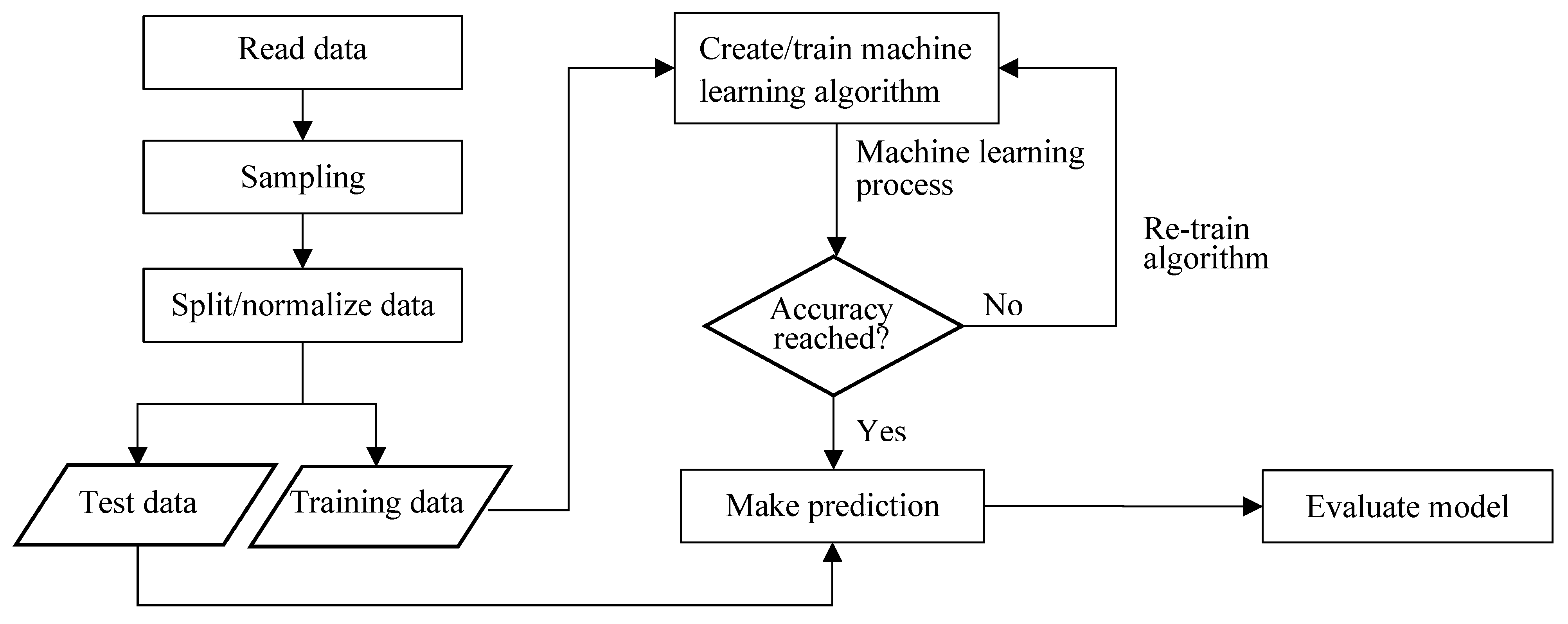
2. Methods

This section describes the methods used in this study (Figure 3).

2.1. Data Processing

The data used in the study were taken from a benchmark database [9]. Four datasets of the ILI records of external defects of pipelines in the United States were collected. Apart from these records, no other information was available about the design and operating parameters of the pipeline, including soil conditions.

The dataset variables and their acronyms are as follows: girth weld number (GWNUM), joint length (in meters), defect’s relative location to the pipe joint (in meters), pipe joint’s longitudinal seam weld orientation (in degrees), not reported in year three dataset; absolute distance of the defect starting point from the origin (in meters), defect starting point circumferential location (in degrees), absolute distance of the defect endpoint from the origin (in meters), not reported year five dataset, defect endpoint circumferential location (in degrees), defect’s most significant point location relative to pipe joint (SIPRD, in meters), defect’s most significant point circumferential location (in degrees), nominal wall thickness (WT, in millimetres), defect length (in millimetres), defect width (in millimetres); defect maximum depth (in millimetres).

The first step in the process was data preparation, where the ILI datasets from the benchmark database were prepared. After removing irrelevant variables and modifying the relevant variables’ names across the datasets, they were merged into one data frame. Then, the data frame was annotated or labelled for later classification of pipeline corrosion defects as per the POF classifications.

2.2. Machine Learning Classification

This section describes the steps used in the machine learning classification process (Figure 4).

Classifying the defects as per the POF category is a non-binary or multi-class classification problem. There are a few machine learning classification algorithms that could be used for supervised learning; these algorithms include decision trees (DTs), ANN, SVM, logistic regression (LR), KNN and Naïve Bayes. Based on the literature review from [11], most learning algorithms used in studies are neural networks, SVM or linear regression.

In building the machine learning models, the data were prepared and are then ready. A sampling technique was applied to the data because of the imbalance. Classifiers, especially SVM, are great for small datasets but take a long time to optimise with cross-validation. Therefore, down-sampling was applied for each class (e.g., pitting, grooving) randomly. All non-relevant columns to defect classification were dropped. Then, the dataset was split into training and test data before the normalisation technique using z-score was performed on the training and test data.

The training data were used to train the machine learning algorithm for learning. The trained algorithm was then fitted with the test data to predict the class of the pipeline defect as per the POF. After that, the machine learning model was evaluated based on the accuracy score as a performance measure.

2.2.1. DT

DT is a supervised learning method used for classification and regression tasks. The “tree” consists of roots, nodes and leaves, which segregate the dataset into different classes based on the values of input features.

The tree is built by recursive partitioning of the feature into subsets based on the values of input features until each division becomes either pure or relatively small. Each partition corresponds to a node in the tree, and each branch corresponds to a decision based on the value of a specific feature. The node aims to split data until the division becomes pure (the data consist of the same class), as measured either by the Gini index or entropy [10].

The DT is grown until all criteria are met, where all data at each node belong to the same class or a maximum depth of the DT is reached. After the model is built, it can be used to predict the new classification or label of the new dataset.

The Gini index is determined as follows:

$$1-\sum _i{p}^2\left(i\right)$$

(1)

where p(i) is the observed fraction of classes with class i. Another impurity measurement is entropy, E. It measures the uncertainty or randomness in a dataset; zero entropy indicates that all the data belong to one class.

$$E=\sum _{i=1}^n-p_i{\log }_{2}p i$$

(2)

One of the limitations of the DT is its tendency to overfit. This issue can be overcome with a random forest model, which involves the construction of numerous trees to give goodness of fit.

2.2.2. Random Forest

Random forest is an ensemble learning method that combines multiple DTs to improve the accuracy of the model. The final decision is achieved by averaging the results of DTs.

Random forest builds multiple DTs on different subsets of training data and input features using a technique called bootstrap aggregating or bagging. In the bagging process, each DT is trained on a random subset of the training samples with replacement to allow several samples to appear multiple times.

The random forest learning algorithm consists of numerous DTs, which comprise bootstrap data samples from the training set. In a classification problem, a majority vote, which is the most frequent categorical variable, will yield the best predicted class.

2.2.3. LR

LR is another machine learning model that can handle binary and multi-class classification problems. For non-binary classification, the approached is called multinomial LR. It models the relationship between the dependent (predictor variable) and independent variables.

The softmax function or maximum likelihood is used to transform the output of the linear model into a probability distribution over possible classes. The output values are between zero and one (Figure 5).

An LR is used for multi-class classification, and it can be expressed mathematically as follows:

$$f\left(y\right)=\frac{1}{1+e^{-x}}$$

(3)

where x is the input to sigmoid function and e is Euler’s number, approximately equal to 2.71828.

2.2.4. SVM

SVM is a supervised learning algorithm used for classification and regression analysis. SVM can be used for linear and non-linear classification tasks and requires a labelled dataset to learn from.

The principle of SVM is to find the best possible hyperplane that separates data into different classes. The selected hyperplane is the line that maximises the margin between two classes while minimising the classification error.

As illustrated in Figure 6, the decision function for linear classification segregates data points based on the maximum margin between support vectors (highlighted in circles). For non-linear classification, the SVM converts the problem to a higher dimension to find the right hyperplane using a kernelling technique.

Three important parameters of the kernelized support vector classifier are the kernel, the “C” parameter and gamma. There are various kernel functions, which are linear, polynomial, radial basis function and sigmoid kernels. For the “C” parameter, low values indicate a low penalty for misclassified points, which results in a higher margin boundary and a greater number of misclassifications. Gamma is a hyperparameter that is used with non-linear SVM where it defines the influence of a single training point. Low values of gamma indicate a large similarity radius, resulting in more points being grouped [21].

In pipeline integrity assessment, SVM is used for defect classification, leakage pre-warning systems, leakage detection and the assessment of defect severity [11].

2.3. Corrosion Growth Rate (CGR)

In determining the short-term CGR, two consecutive ILI data sets (i.e., Year 7 and Year 5) were matched using Pandas’ method of merging data frames on the GWNUM and SIPRD. For the long-term CGR, the difference was calculated from the first and latest inspection datasets over 6 years.

2.4. Remnant Life Analysis

One of the industry practices is adopting a deterministic approach of defining one corrosion growth for each corrosion defect using a single value, linear or non-linear model. However, this approach is conservative and impractical without considering the uncertainty of the corrosion process. Conversely, a probabilistic approach for determining the pipeline burst pressure considers the uncertainties of random variables.

Several industry codes and best practices, such as American Society of Mechanical Engineer (ASME) modified B31G, SHELL92 and DNVGL-RP-F101, are available. Modified B31G is the most preferred in the industry because of its accuracy. These deterministic methods are used for predicting the pipeline’s remnant life by burst pressure, Pb, which can be computed as follows [18]:

$${\mathrm{P}}_{\mathrm{b}}^{\mathrm{A}\mathrm{S}\mathrm{M}\mathrm{E}}=\left\{\frac{2t}{D}\right.\left(1.1{\mathsf{\sigma }}_{\mathrm{y}}\right)\mathrm{*}\left[\frac{1-\left(2/3\right)\left(d/t\right)}{1-\left(2/3\right)\left(d/t\right)M^{-1}}\right]\hspace{1em}\hspace{1em}if l^2/Dt\le 20$$

(4)

$${\mathrm{P}}_{\mathrm{b}}^{\mathrm{A}\mathrm{S}\mathrm{M}\mathrm{E}}=\left\{\frac{2t}{D}\right.\left(1.1{\sigma }_y\right)*\left[1-\left(d/t\right)\right]\hspace{1em}\hspace{1em}if l^2/Dt>20$$

(5)

where D is the pipeline diameter; t is the wall thickness; l is the defect’s length; d is the defect’s depth; σ_y is the yield strength; and Folias Factor (M) = √(1 + 0.8(l/D)²(D/t).

Probabilistic Analysis

Probabilistic analysis is commonly used in pipeline corrosion prediction to assess corrosion-related failures and determine the suitable remedial action. Statistical methods and simulation techniques, such as MCS, are used to analyse the probability distributions and generate a range of potential corrosion scenarios.

Statistical probability distributions, such exponential, normal, Gamma, Weibull, Gumbel, Cauchy and lognormal, were applied for random variables of the burst pressure in the Phyton programming.

The probability of failure (PoF) can be computed based on a generic reliability equation as follows [18]:

$$R=P\left[g\left(X\right)>0\right]=\int \dots \underset{g\left(X\right)>0}{\overset{}{\int }}{f}_x\left(x\right)dx$$

(6)

where $f_x$ is the joint probability density function of the n-dimensional vector x and g is the state limit function $({g=P}_b-P_o)$. P_o is the pipeline operating pressure. The probability of the pipeline is in a safe state if g > 0 and in a failure state if g ≤ 0.

3. Results

This section provides the results, which are divided into four sub-sections: data visualisation, machine learning, CGR and remnant life analysis.

3.1. Data Visualisation

The combined data frame of all four ILI datasets has about 3.2 million records (rows) and 16 columns. The pipeline reference wall thickness (t) is 7.1 mm. Hence, 10 mm was used for the WT (A) (please refer to Figure 1b).

Figure 7 visualises the massive ILI datasets. Figure 7a shows that the counts of defect dimension class by the inspection year indicate an increasing trend for pitting, axial grooving and axial slotting corrosion. However, the trends reversed from year 3 for general and circumferential grooving, which can be attributed to the remedial works carried out by the pipeline operator, such as sectional pipeline replacement.

The distribution of significant defect orientations in Figure 7b has two peaks. The majority of external corrosion defects occurred at the orientation between 80–150° and 200–260°.

3.2. Machine Learning Classification Models

In this section, machine learning classifier models, such as DT, SVM and LR, were built for multi-class classification. The accuracy of each model was used as a performance measure using the train and test method. The Year 7 ILI dataset was used because it had adequate samples for all the corrosion defect classes.

The dataset was split into training and testing datasets with an 80:20 ratio before being normalised.

Table 1. Statistics of normalised train and test datasets.

Feature (mm)	Type	Count	Mean	Std	Min	25%	50%	75%	Max
Length	Train	5600	29.93	41.97	5	9	19	32	724
Width	Train	5600	38.39	66.57	5	9	16	43	1472
Length	Test	1400	29.47	41.04	5	9	20	32	746
Width	Test	1400	38.87	63.60	5	9	16	45	590

summarises the statistics of the normalised train and test datasets.

The model accuracies are ranked in

Table 2. Accuracy Score and Computational Time of Machine Learning Classifier Models.

Machine Learning Model	Accuracy (%)	Time (s)
Decision Tree	99.9	0.00
Random Forest	99.8	0.01
SVM Radial Basis Kernel	92.3	0.50
SVM Linear Kernel	90.3	0.23
Logistic Regression	90.0	0.00
SVM Sigmoid Kernel	76.5	0.36
SVM Polynomial Kernel	67.0	0.31

. The best classifier model is the decision tree that is the most accurate and fastest in computational time.

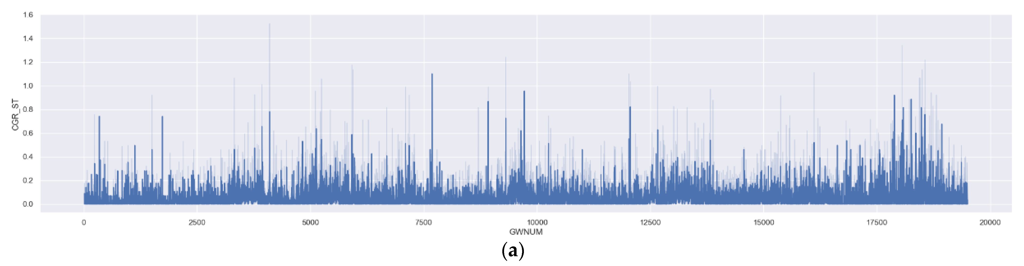
3.3. CGR

ILI matching of the Year 5 and 7 ILI datasets were merged using GWNUM and SIPRD as references. This approach resulted in 202,378 defects that were matched for short-term corrosion growth analysis. Negative CGRs were removed, leaving 136,200 records.

For long-term CGR analysis, the first and latest inspection datasets were matched using the same approach, which resulted in 3241 positive CGR rates.

Table 3. Top 5 short-term corrosion growth rates.

GWNUM	SIPRD (m)	CGR (mm)
18740	5.25	2.27
15319	9.89	2.24
15165	9.85	2.02
5806	7.12	1.95
13475	11.13	1.92

ranks the highest short-term CGR along the pipeline.

Figure 8 indicates the distribution of CGRs by the pipeline GWNUM.

3.4. Remnant Life Analysis

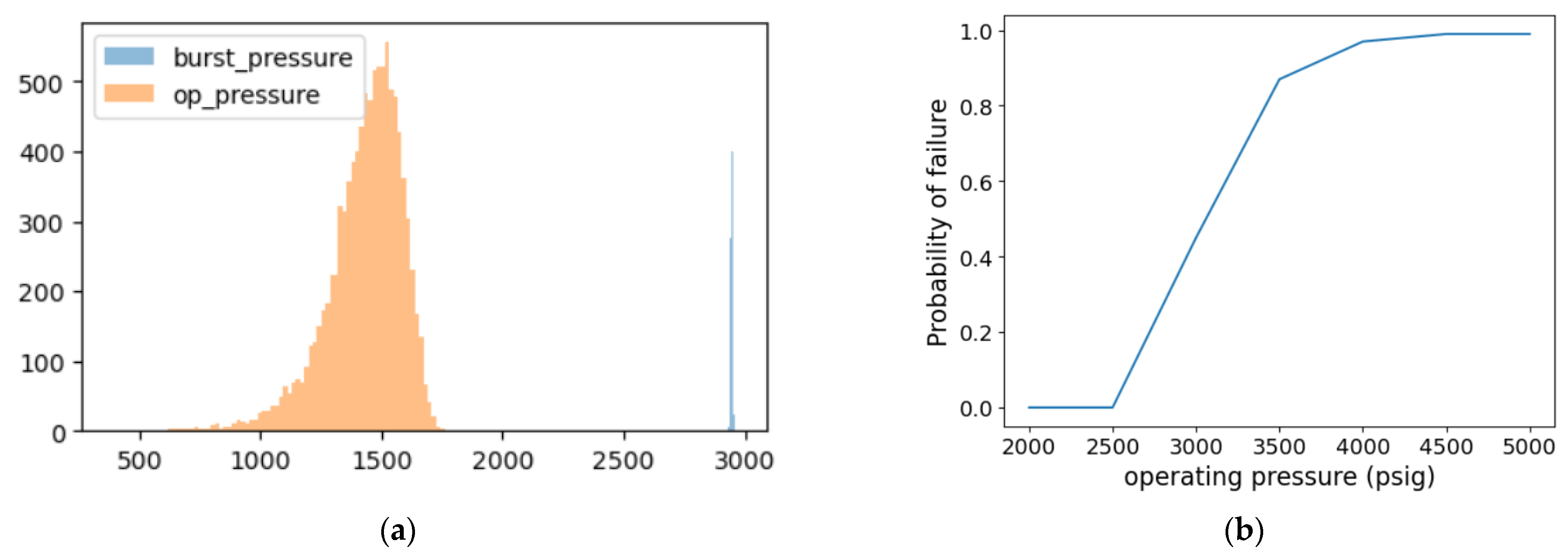
In this part, the burst pressure of the pipeline for individual defects was calculated as per ASME B31G code Equations (1) and (2). Figure 9a depicts the distribution of burst pressure for all datasets, which is a deterministic method, with the mean value at 2937 psig.

For the probabilistic MCS, uncertainties were considered to estimate the PoF when the pipeline operating pressure exceeded the burst pressure of the corroded pipeline.

Running an MCS involves two components: the equation for evaluation and random variables for the input. Random variables were generated and burst pressure was calculated again using Equations (1) and (2). Figure 9b summarises the PoF for a different operating pressure.

The pipeline parameters were unavailable in the original dataset; therefore, the user-defined values were obtained from the literature [18] as per

Table 4. Probabilistic models of the random variables [18].

Variables	Pop (psig)	D/mm	t/mm	l (mm)	d/mm
Type	Gumbel	Normal	Normal	Normal	Normal
μ	1500	273.1	7.1 *	50.7 *	0.33 *
COV	0.08	0.001	0.001	0.001	0.001

* Actual data.

below.

4. Discussion

Categorisation of pipeline corrosion defects is a multi-classification problem. The features of the ILI dataset, which include a defect’s length and width and the pipeline’s nominal thickness, were selected based on the POF.

Based on the results of classifier models in Section 3.2, DT is the most accurate and requires very little computational time. The second most accurate model is the random forest model, which is an ensemble method. SVM classifiers with different kernels require considerable processing time for the whole training dataset due to cross-validation. This issue was overcome by down-sampling for the imbalanced dataset.

Another deep learning model, which is the ANN, was experimented on. This type of model is normally used for image classification or time-series predictions. Its computational time was significantly higher than that of the machine learning methods discussed above, and it achieved 98.5% accuracy (not tabulated in the Section 3). Meanwhile, given its lower accuracy and longer computational time, the deep learning model was not recommended for the ILI dataset, which was in a tabular format. Instead, machine learning models, such as DTs and random forest, performed better.

Another aspect that can be considered for future study is tuning the hyperparameters of models, such as the maximum depth of the tree or the number of trees in the forest. For SVM, optimisation methods, including finding the optimal value of the regularisation parameter (C), control the trade-off between maximising the margin and reducing the misclassification error.

In addition, the dataset was split into training and testing datasets. Training performance can be further evaluated to prevent the over-fitting issue from arising. This goal can be achieved by splitting the testing dataset into test and validation sets.

In ILI matching, the defect’s orientation was not considered. If considered, the remaining dataset would have been further reduced to about 9000 records. The rationale for dropping the defect’s orientation was to consider that the inspection gauge orientation may shift during pigging operations. Alternatively, a probabilistic matching approach such as that in [14] can be used to reflect uncertainty in the matching process.

In calculating the CGR, this study considered only individual defects. The interaction between nearby or grouping defects was not considered, which could be expanded for future studies.

Finding the best-fitted distributions for all random variables is a challenge. Several distributions, such as normal, beta, exponential, gamma, logistic, lognormal, Cauchy, Weibull and Gumbel distributions, were fitted to the variables. When a Kolmogorov–Smirnov test was applied for the goodness-of-fit, the p-values were zero for all distributions. Therefore, the results are inconclusive. Other approaches to finding the best-fitted distribution can be explored with different methods of identifying parameters, such as sum-square error, Akaike Information Criterion (AIC) and Bayesian Information Criterion.

5. Conclusions

As oil and gas operators are currently facing enormous challenges in organising and analysing data for managing asset integrity due to the volume, variety, velocity and veracity of data, the adoption of digitalisation, including machine learning approaches, will facilitate the decision-making process. This step will not only assist pipeline engineers, but will also enhance the integrity of pipeline management systems and, in return, unlock more value to organisation. The benefits are increased efficiency, time saving and reduced human errors.

This study is framed to help automate tedious tasks of pipeline integrity engineers in defect matching and its reliability analysis. This work features several limitations, including the availability of the design and operating parameters of the pipeline, and historical records of maintenance activities, such as repair and replacement. These limitations influence the outcome of the ILI matching process and, subsequently, the CGRs and remnant life analysis. Another limitation of this study is that the interaction of corrosion defects and the influence of soil condition on the external CGR where the pipeline is buried were not considered. These limitations are not within the scope of this study. For future research directions, the scope of this study can be extended to consider the interactions of corrosion defects and the tuning of hyper parameters of machine learning classifier models.

In conclusion, the realisation of continuous real-time pipeline corrosion monitoring technology is possible considering that existing limitations are addressed and resolved systematically for the enhancement of pipeline integrity management. The adoption of machine learning approaches in classifying pipeline defects as per POF requirements and matching ILI data for determining the CGR and remnant life of pipelines can help the oil and gas industry in predicting future outcomes more accurately and planning for unknown events to avoid consequences of failure, which can be catastrophic due to the potential hazard to human health and safety loss.