

Assessing the Performance of Small Wind Energy Systems Using Regional Weather Data


Institute of Mechanical, Process and Energy Engineering, School of Engineering and Physical Sciences, Heriot-Watt University, Edinburgh EH14 4AS, UK
Energies 2023, 16(8), 3500; https://doi.org/10.3390/en16083500
Submission received: 3 March 2023
/
Revised: 6 April 2023
/
Accepted: 12 April 2023
/
Published: 17 April 2023
(This article belongs to the Topic Advances in Wind Energy Technology)
Abstract
:While large renewable power generation schemes, such as wind farms, are well monitored with a wealth of data provided through a SCADA system, the only information about the behaviour of small wind turbines is often only through the metered electricity production. Given the variability of electricity output in response to the local wind or radiation condition, it is difficult to ascertain whether particular electricity production in a metering period is the result of the system operating normally or if a fault is resulting in a sub-optimal production. This paper develops two alternative methods to determine a performance score based only on electricity production and proxy wind data obtained from the nearest available weather measurement. One method based on partitioning the data, consistent with a priori expectations of turbine performance, performs well in common wind conditions but struggles to reflect the effects of different wind directions. An alternative method based on Principal Component Analysis is less intuitive but shown to be able to incorporate wind direction.
1. Introduction
While industrial-scale wind energy projects using MW-scale turbines have grown rapidly over the last two decades, smaller wind turbines have grown at a much slower rate and somewhat stood in the shadow of utility-scale wind energy. However, they play an important role in supplying energy to smaller and rural communities, as well as for embedded generation in sub-urban and even urban environments [1] in highly developed countries as well as bridge economies and developing countries [2]. However, the operating characteristics and resulting productivity and cost-effectiveness are highly variable, as shown by a detailed analysis of 43 turbine models available in 2011 [3] and a detailed comparison of potential productivity across the UK [4]. In terms of their cost-effectiveness, small wind turbines are at an inherent disadvantage over the large wind energy market since they cannot exploit economies of scale while also operating closer to the ground where the wind is always lower than higher in the atmosphere. Some years ago, it was found that even in good locations in the UK, there was no financial benefit of micro wind turbines with payback periods in excess of 25 years [5]. Since then, the economic conditions have changed, and an analysis of the levelised cost of energy (LCoE) for a range of settings [6] has shown that the LCoE for a small wind turbine installation can range from only three times the typical LCoE for utility-scale onshore wind farms to a factor of almost 30 higher [7]. Therefore, it is even more important to design or select the most suitable turbines, install them in the best location for them, and then ensure that they operate as well as they can.
This translates into three major specific challenges for small-scale wind: the first is related to the turbine design [8], as the smaller wind turbines need to be designed for more turbulent and volatile wind conditions than larger turbines whose rotors are placed much higher in the atmosphere. While the design of large turbines has largely converged to an industry standard of a variable-speed, pitch-controlled, three-bladed upwind horizontal-axis wind turbine, the design of small wind turbines is still much more diverse [9]. Given their typical placement, the turbulence characteristics, especially in urban environments, are very different from those described by IEC standards developed for larger turbines [10]. Therefore, the capture of the turbulent component in the wind is more important than for larger turbines [11], where tuning the response of the device to the turbulence spectrum in its environment can increase the power conversion significantly [12] and, therefore, overall productivity [13].
The second challenge is the optimum micro-siting of turbines, as the local wind conditions vary significantly across a small area. For example, the performance of a roof-top mounted turbine varies substantially for different points on the roof, as demonstrated for a regular array of detached houses with a pitched roof in a staggered layout for wind perpendicular to the roof ridge [14] and a non-staggered layout for a range of roof shapes and wind directions [15]. While this is a challenge, identifying suitable locations in an urban environment also opens up possibilities to exploit locations where the wind is channelled and augmented [16]. An investigation of the performance and market potential of pole-mounted horizontal-axis turbines installed across the UK, commissioned by the UK Government [17], illustrated that challenge but also highlighted the fact that for most of these turbines, the only available information was the metered electricity without information about the local wind conditions.
This is the third challenge, namely monitoring and effective maintenance of smaller wind turbines. Large turbines are fitted with a large number of sensors to monitor environmental and turbine conditions [18] gathering large volumes of data through a SCADA system, e.g., [19], with much research into analysis methods, e.g., [20]. Smaller turbines, on the other hand, are often not monitored except through the electricity meter monitoring the electricity production accumulated over an accounting period, commonly at half-hourly intervals or even less frequently. In response, a field trial was set up to monitor a selected set of turbines across the UK with additional instrumentation to gather local wind speed and turbine power output at a 5-min interval [21] and to compare the findings of the monitored and unmonitored turbines to wind speeds from nearby meteorological weather stations. Results were only reported as annual data, but they still show some correlation between the local wind measurements and the weather station. That was a funded field trial using costly anemometers, but such instrumentation is impossible for an economically viable installation of such small wind turbines. This requires either much cheaper monitoring equipment [22] or a way to infer performance information from other sources. Despite a careful search of the literature, the author has not found research or guidelines on a protocol for evaluating small wind turbines once they are installed other than site visits, be they for planned maintenance or once a fault has been noticed.
1.1. Turbine Performance Modelling
The first step setup in monitoring turbine performance is to create an appropriate model of the turbine’s (or turbines’) performance in their installation setting. Manufacturers only provide a single-valued performance curve of power output for a set of reference wind speeds. Determining even such a curve empirically has attracted much research, e.g., [23]. However, actual operating turbines show visible scatter around that curve even in simple surroundings, such as offshore wind farms [24]. That scatter is significantly enhanced in complex terrain, leading to a challenge in performance modelling even with dedicated wind speed and directions measurements at the turbine site [25].
Given the nonlinear nature of a turbine’s performance curve, one immediately intuitive approach is to partition the data into different segments. This could be used to construct a single curve [26] or a distribution within each partition. With the surge in AI and machine learning, artificial neural nets have also been applied to this subject [27]. Out of a range of statistical methods, copula theory has been applied to develop a model of wind turbine performance [28] to construct the joint probability of power output and wind speed from operational data. This could be applied as a benchmark to compare new measurements again for performance monitoring. However, it is unclear how this would be extended to incorporate other factors, such as wind direction.
Principal component analysis (PCA, see [29] for a detailed introduction and [30] for examples) is a technique which is widely applied for the reduction of data complexity or dimensionality by projecting the multi-variate data onto empirical orthonormal reference basis vectors, with the leading basis vector capturing the largest contribution to the overall variance and the following vectors successfully less variance. The data reduction is then applied by retaining only a selected number of dimensions to be able to reconstruct a filter data set which maximises coherent signal and minimises noise. This has been applied for wind turbine performance modelling using a number of wind speed measurements at different heights above ground at the turbine site together with the turbine power output [25]. Other applications for wind energy problems include forecasting, proposed by [31] and further developed by [32], using time-delay PCA, also known as singular systems analysis [33].
PCA has also been shown to be a useful technique for analysis of spatially distant measurements [34], in that case, as a measure-correlate-predict (MCP) method for wind resource assessment. There, the PCA combined the time-aligned measurements of wind speed from pairs of anemometers, where the distance between the anemometers varied from about 10 km to around 100 km, and the data covered a period of 12 years. In the MCP algorithm, the PCA predictor was trained on the pair of readings from a training period of 1 or 2 years. That predictor was then used to infer the wind speed and direction at one of the pairs for the remaining data period using the measurements from the other anemometer only. That method was shown to be consistently superior to a standard MCP using linear regression. With this, there is clear evidence that PCA can be used to extract key information from input data combining either wind speed and wind power at the same location [25] or spatially distant data but only using wind data (and not wind power) [34]. Based on this evidence, it can be postulated that PCA might be similarly able to extract a useful mapping between wind power at one location and wind speed some tens of kilometres apart. The degree to which this hypothesis holds will be given by the scale of the weather patterns, which lead to a general spatial correlation that has a clear functional dependence on the distance [35].
1.2. Aims and Objectives
The aim of this paper is to develop methods to monitor and evaluate the performance of a set of small turbines using only the metered electricity production together with wind speed and direction data from a ’nearby’ weather station, where nearby could be several 10s of kilometres from the turbines. To this end, the objectives of this study are to develop turbine performance models using a training data set, to apply the model to a later set of validation data, and to develop a monitoring metric for the judgement of the performance. Given the lack of existing methods to provide feasible near-online monitoring of small wind turbines, the scope of this work has to be limited to the proof-of-concept stage to demonstrate its potential and to identify clear steps to develop the method towards practical application.
Two complementary turbine models are here developed, one based on the a priori expectation of the empirical performance curve being close to a typical manufacturer’s curve by partitioning the data into wind speed bins and analysing the observations within each bin. The second method is entirely data-driven and trains a model using principal component analysis, as this has been proven to be a valid tool not only for co-located multi-variate data [25] but also for spatially distant data [34].
The rationale for developing two independent methods is two-fold. First, the absence of any available state-of-the-art method or protocol presents a major obstacle to validating any single method developed here against an external benchmark. However, the two methods, which in their approach are fundamentally different, can be used to provide some cross-validation of each method. The second reason is that the two proposed methods have complementary advantages and disadvantages. The first method is by its nature more intuitive as it is based on the known concept of a wind turbine performance curve, while the other is purely data-driven and therefore not directly tied to a priori knowledge. However, the use of the performance curve poses challenges when secondary information such as wind direction is to be included in the algorithm, while the multi-variate PCA method can be applied to any choice of input variable combination.
The methods will be illustrated for metered electricity production from an installation in Scotland, together with wind data from the nearest routinely maintained UK Meteorological Office weather station. The data and methods are introduced in the following section, with the results from each section presented in Section 3, followed by a comparison and discussion in Section 4, before a brief conclusion with some suggested further steps.
2. Materials and Methods
Given the constraints of minimal monitoring data and no extensive initial validation of performance after installation, the method proceeds in two stages utilising a small set of input variables only: at the very minimum, only the metered electricity production and the wind speed from the nearest weather station, or additionally the wind direction as a third variable. The first step is the creation of a training data set which has been carefully screened to increase the confidence in that the training data set does not contain faulty performance. This training data set is then used to develop a reference performance model against which future operational data can be bench-marked. To provide a benchmark metric, a performance score is defined.
The overall process is structured in the following distinct steps, with reference to the sections where the method or its application is introduced:
- 1.
- Creation of a training data set and a validation data set (Section 2.1)
- (a)
- Splitting the full data set into one full year of data for training and retaining the remainder of the period for validation
- (b)
- Carefully screening of the training data set for known times of turbine or grid faults and remove those
- (c)
- Checking the remaining training data for potential bias arising from data gaps
- 2.
- Method 1, based on the performance curve (Section 2.2)
- (a)
- Creation of an empirical performance curve from the training data (Section 2.2.1)
- (b)
- Definition of a performance score function with reference to the empirical performance curve (Section 2.2.2)
- (c)
- Application of that performance score function to the validation data to calculate a score for each validation sample (Section 3.1)
- 3.
- Method 1a, incorporating wind direction (Section 2.2.3)
- (a)
- Identification of a partition of the data using wind direction from training data
- (b)
- Subdivision of all data into the appropriate directional data partition
- (c)
- Creation of empirical performance curves for each directional partition from the training data
- (d)
- Definition of a performance score function for the empirical performance curve in each directional partition
- (e)
- Application of the partition-appropriate performance score function to the validation data to calculate a score for each validation sample (Section 3.1)
- 4.
- Method 2, using PCA (Section 2.3)
- (a)
- Creation of the reference performance in PCA space from the training data (Section 2.3.1)
- (b)
- Definition of a performance score function with reference to the PCA reference (Section 2.3.2)
- (c)
- Projection of the validation data onto the PCA space (Section 3.2)
- (d)
- Application of the performance score function to projected validation data to calculate a score for each validation sample (Section 3.2)
- 5.
- Method evaluation
- (a)
- Cross-method comparison by comparing the performance scores from each method as an initial validation of the methods (Section 4.1)
- (b)
- External validation (Section 4.2)
- (c)
- Demonstration of how the methods could be used to identify potential performance improvement (Section 4.3)
2.1. Data Availability and Quality
The data available are half-hourly-metered electricity production from an installation complemented by hourly wind speed and direction data for the same time period from a nearby weather station operated by the UK’s meteorological office.
2.1.1. Electricity Production Data
The wind energy data used to develop and illustrate the method were provided by the owner of an installation on an island in the north of the UK. The installation consisted of three 5 kW turbines with a nominal rated wind speed of 13 m/s. They were mounted on 15 m tall poles and had upwind horizontal-axis rotors, passively yawed through a vane. Just over two years of data are available, from July 2013 to July 2015, with one extended gap of 43 days in November and December 2013 and a shorter gap of 6 days in February 2014.
2.1.2. Weather Data
The nearest weather data are taken from a UK Meteorological Office land-based weather station near an airport that is located 25 km to the south of the wind turbine site. These data were obtained through the MIDAS data set [36]. This data set provides hourly average wind speed and gusts in a 10-min measurement period leading up to the measurement time stamp, both rounded to the nearest knot, and the wind and gust directions rounded to from an anemometer at a nominal height of 10 m above ground. A preliminary analysis showed that there is a very close linear relationship between the recorded mean wind speed and gusts such that with a correlation coefficient of . A check of the wind speed distribution of these data against that of a 12-year record for the same weather station suggests that the winds observed within each year are consistent with the long-term climatology. Implications of either including or excluding rare wind conditions, and how to mitigate this, will be addressed in the Discussion in Section 4.4.
2.1.3. Data Alignment
The available installation performance data were only the metered electricity fed into the grid with a half-hour resolution. To maintain the data resolution of the key variable, namely the electricity production, the weather data were augmented. Since the weather data are directly valid for the 10 min prior to the full hour, the direct weather station data were used as the correlates for both the half-hour leading up to that full hour and the half-hour period immediately following.
The wind speeds recorded during the gaps in the electricity data do not show any unusual distribution and certainly do not include any extreme weather events which might have affected the turbines’ behaviour in ways not described by the manufacturer’s performance curve. As a result, the data gaps are inferred to be due to communications issues and not linked to the wind resource. With a data availability of 93.5%, it can be assumed that the gaps will not introduce a significant bias in the analysis and are simply ignored in the analysis. This is possible since the analysis is purely based on temporally independent samples of simultaneous measurements.
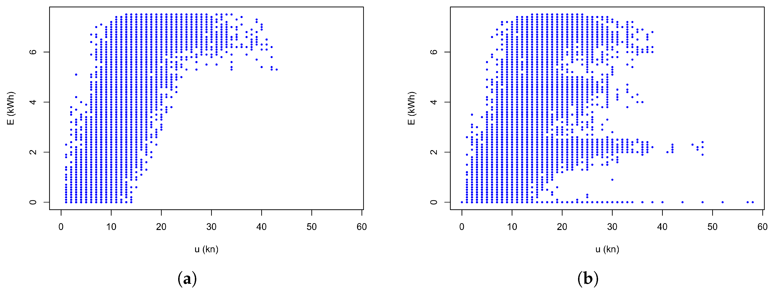
In the second step, the full data set was separated into two sets, each covering about a year, with both sets shown as simple scatter plots of the electricity production against the time-aligned wind speed in Figure 1. The first year was screened for known problems, such as recorded down times of turbines. The remaining data in the first year were then deemed to represent only the ’normal’ operation of the installation and were then used as the training data set. The second year of data was taken without screening. The training period shows a clear organisation around a typical wind turbine performance curve, reaching a maximum output of 7.5 kWh at a wind speed as early as 10 kn but with a substantial scatter. The later validation period, in Figure 1b, shows additional features which clearly suggest that for a number of times, one or more of the turbines were not generating, as well as some data which fall in between these distinct bands. This comparison of the two separate years shows clearly that there are a number of instances in the second year which do not conform with the established expectations from the first year, in some instances because turbines are disconnected completely but in other, less clear, instances where all turbines are operating but with a lower output than they could. The purpose of the methods developed here will be to identify those instances as soon as the data become available. The score at times, which are clear-cut, should identify a clear fault, but the score should also indicate potential problems in the other cases.
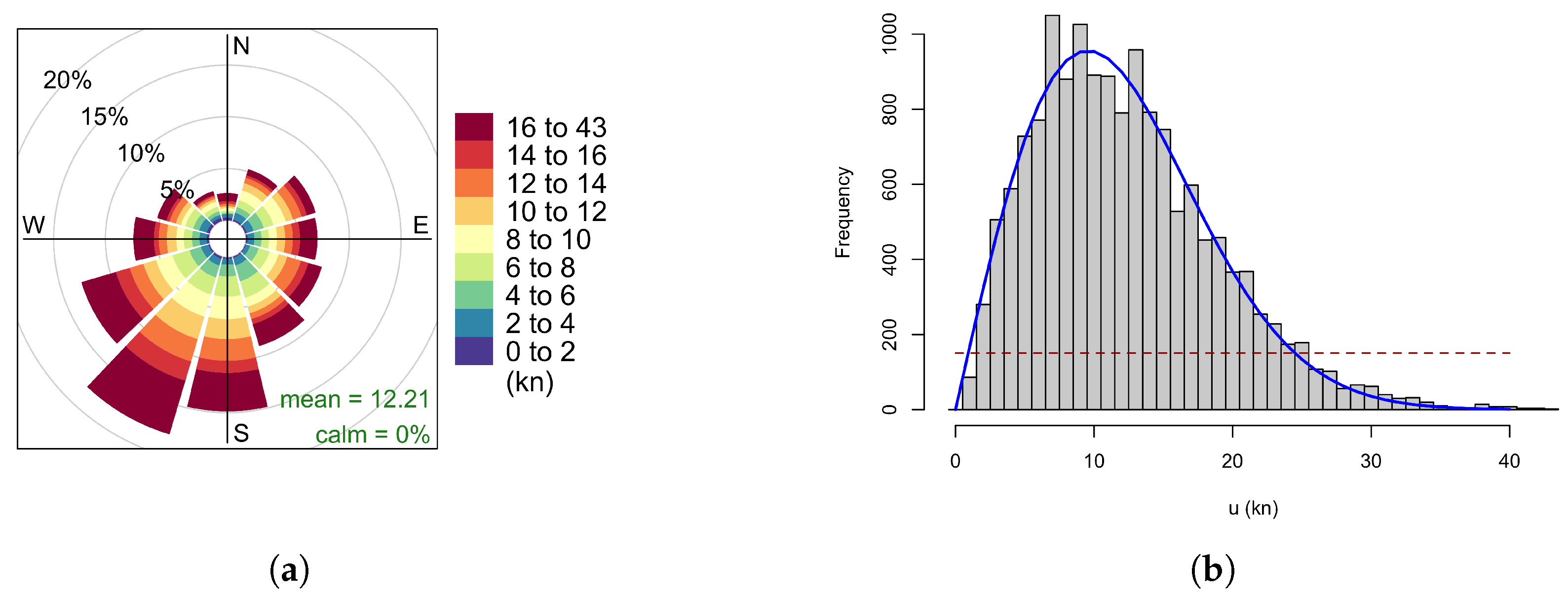
For the training period, the wind rose in Figure 2a shows the pattern typical for the UK with prevailing south-westerlies, and a wind speed distribution in Figure 2b approximating a standard Weibull curve with a scale factor of kn and a shape factor of . While some wind speeds have been observed around 1000 times, other wind speed bins have less than 100 samples.
2.2. Method 1, Based on the Performance Curve
2.2.1. Creation of a Reference Performance Curve Using Data Partitioning
The first step in the creation of the reference performance curve for the installation is to split the data from Figure 1a into wind speed bins. Since the wind speed is given in integer knots, this is the natural binning. After this, the electricity production data in each wind speed bin have to be separated into ’normal’ and ’unusual’ behaviour. In the absence of independently gathered information on the turbine’s performance, this is necessarily a somewhat subjective distinction and requires expert interpretation of the wind speed distributions. For this analysis, a choice was made to consider the central core of 50% of the observations in Figure 1a as the main reference performance curve and the shoulder areas as acceptable, with the implication that the blank areas below this curve should be regarded as unacceptable.
2.2.2. Definition of a Performance Score
The desired performance indicator or score, S, should result in a reference value for standard performance, a low score for performance clearly below standard and a high score for performance exceeding expectations. This is satisfied by a function which has three main levels: 1 for standard behaviour, 0 for performance clearly below standard, and 2 for exceptionally good behaviour. This could either be a discrete three-level function or a piece-wise linear function with these three levels and linear interpolations in between.
The approach taken here was to classify the two central quartiles as representing standard performance with a score of 1. The lowest quartile was classified as a transition region where the score would drop from ’normal’ to clearly faulty (score of 0) in a gradual way. The top quartile was similarly regarded as a region where the turbines were performing increasingly better than one could expect. To quantify this classification, the quartiles for the electricity production, E, within each wind speed bin, , were calculated as to , or to in short. The position of a data point within the sample was then used to create a performance index as
The subscript is used to indicate that this definition is for the ’simple’ performance score and to distinguish it from the directional score defined in Section 2.2.3 and the PCA score definition developed in Section 2.3.2.
2.2.3. Method 1a Incorporating Wind Direction
As it is known that the wind direction will affect the relationship between the local wind at the installation and the reference anemometer, especially in the wind speed range from cut-in to a little above-rated wind speed [24], this can be used to refine the performance judgement. The process outlined so far is refined by splitting the samples within the wind speed bin into distinct wind direction sectors. To retain sufficient data within each analysis sub-bin, it was not possible to carry this out for each wind direction bin or even a section covering several bins. Instead, the individual wind directions were grouped into a small set of groups according to their average productivity within the entire wind speed bin. This would start with separating the wind speeds into two groups, one giving electricity production above average and the other below. The next refinement would be three groups, one additional group for the intermediate range.
The performance indicator for the directionally sub-divided data, , is calculated in the same way as in Equation (1) but using the quartiles appropriate for the wind direction group in their respective wind speed bin, .
As mentioned in Section 2.1, the wind data also include gust speed and direction. Incorporating this additional information into this method is impossible without having many empty partitions. However, a method which does not rely on partitioning data into pre-defined subsets might allow additional data to be incorporated without running into this problem.
2.3. Method 2: PCA-Based Score
While the method outlined in Section 2.2 follows a clear, rational argument underpinned by the knowledge of the typical shape of a turbine’s performance curve, incorporating the directional information leads to insufficient data samples available within a reasonable training period. To alleviate that problem, an alternative method is developed here, which incorporates the directional information implicitly without sub-sampling the training period.
2.3.1. Creation of the Reference in PCA Space
This method is based on a Principal Component Analysis, PCA, of the training data, which have been combined into a matrix of column vectors of the three variables, each normalised to be in the interval ,
with , and . The PCA is carried out by a Singular Value Decomposition of that matrix (If the matrix is too large for a direct Singular Value Decomposition, an alternative is to carry out an Eigenvalue Decomposition of the much smaller covariance matrix, ).
with
- a matrix containing the column vectors of the principal components, also known as the ’loadings’ or components in a row to reconstruct the input sample in the same row in ;
- a diagonal matrix of the singular values, each measuring the contribution to the total variance of its corresponding singular vector;
- a matrix containing the column vectors of the singular vectors, which form an orthonormal set of basis vectors rotated with respect to the original basis vectors to maximise variance in the leading basis vector (Note that some software packages have implemented Singular Value Decomposition such that they return the singular vectors as row vectors, such that the singular vector matrix is the transpose of that described here).
The principal components fill a volume within the space spanned by the singular vectors, and new measurements can be projected onto the same space. If a measurement is projected onto a location also occupied by some training samples, this indicates that the new measurement is consistent with the training data. If, however, the new measurement is in an empty part of the space, it would not be consistent with the training data. This case would either indicate previously unseen weather conditions or previously observed weather conditions associated with unexpected turbine productivity.
This projection of a new measurement (or set of samples) is carried out by applying the scaling using and from the training to the new measurements, , and then inverting Equation (2) to
where since it is an orthonormal matrix, and the inverse of is the diagonal matrix with elements .
2.3.2. PCA Performance Score
To add some gradation to that distinction of within and outside, the volume delineated by the training data, the space can be subdivided into volume elements, , and the number of observations within a volume element gives a measure as to whether it is within the core of the volume or a less densely populated region. This sample density can be used to provide a continuous measure as to how well the new observation conforms with the expected behaviour.
One has to bear in mind that this number of observations is the result of the joint probability of some weather conditions occurring at the anemometer site and some electricity production being observed at the turbine site, . However, the performance measure has to be based on the conditional probability distribution of electricity production given a particular wind condition. To construct this conditional electricity probability, the joint probability has to be divided by the weather condition distribution. While this would itself be a joint probability distribution of wind speed and wind direction, a reasonable first approximation in the approach is to use the wind speed distribution alone since the wind direction is likely to have only a secondary effect on the turbine’s productivity. This is easily obtained from the training data, either by creating a histogram or fitting a Weibull distribution as presented in Figure 2b.
At extremely low and high wind speeds, however, the wind speed distribution is very low, and any uncertainty or noise in either the PCA density or the wind speed distribution would be amplified. To avoid this, the division using the wind speed distribution has to be capped at a minimum value, commensurate with the overall sample size and distribution of sample densities. Hence, a measure proportional to the conditional probability can be calculated by dividing each sample in a PCA volume element by the probability of the wind speed associated with that sample. An equivalent option is to divide with the direct count, of that wind speed (cf. Figure 2b), subject to replacing low numbers by the set minimum with
where is the number of observations with wind speed u. In the present work, with 15,044 samples in the training data set, the minimum was set as 1% of the total number, that is indicated as the dashed horizontal line in Figure 2b. The wind speed bins affected by this cap are the lowest observed wind speed of 1 kn and all high wind speeds above 25 kn.
Given the available data volume, it was decided here to apply this principle to the projection of the data onto a selected plane, which, with inspection, was guided to be the plane. This reduced the volume elements to area elements and counted all samples within that volume for all values of . Taking the set of samples within the volume as K, the conditional probability is proportional to the count of each sample weighted through division by ,
This could be easily normalised into a probability density function, but its purpose is to construct a performance score corresponding to that developed in Section 2.2.1, Equation (1). To this end, is transformed into a piece-wise linear form, with the entire set of routinely acceptable performance from the training data receiving a score of 1. This is achieved by first setting a reference threshold consistent with the choice of the interquartile range designated as core performance. Therefore, the median of , denoted by , was chosen as the threshold. The value of is first divided by , and then all values above 1 are set to a value of 1,
This leads to the most likely electricity production volume in the PCA space having a score of , volumes not being part of the training data having a score of , and the space in between an intermediate value. As this does not distinguish between ’better than expected’ and ’worse than expected’, the PCA volume has to be subdivided into the space associated with high electricity production and its complement associated with low electricity production. The values in the high-electricity subspace are then mirrored around the reference score of 1 by subtracting the initial score from a value of 2; those initially with a value of 0 become 2, while those originally with a value of 1 retain that value. This finally leads to a score equivalent to that defined in Equation (1) with
3. Results
The presentation of the results essentially follows the same structure as Section 2, starting with the simple quartile-based performance index, followed by including the effect of wind direction, and concluding with a demonstration of the PCA-based scoring.
3.1. Method 1: Quartile-Based Performance Index
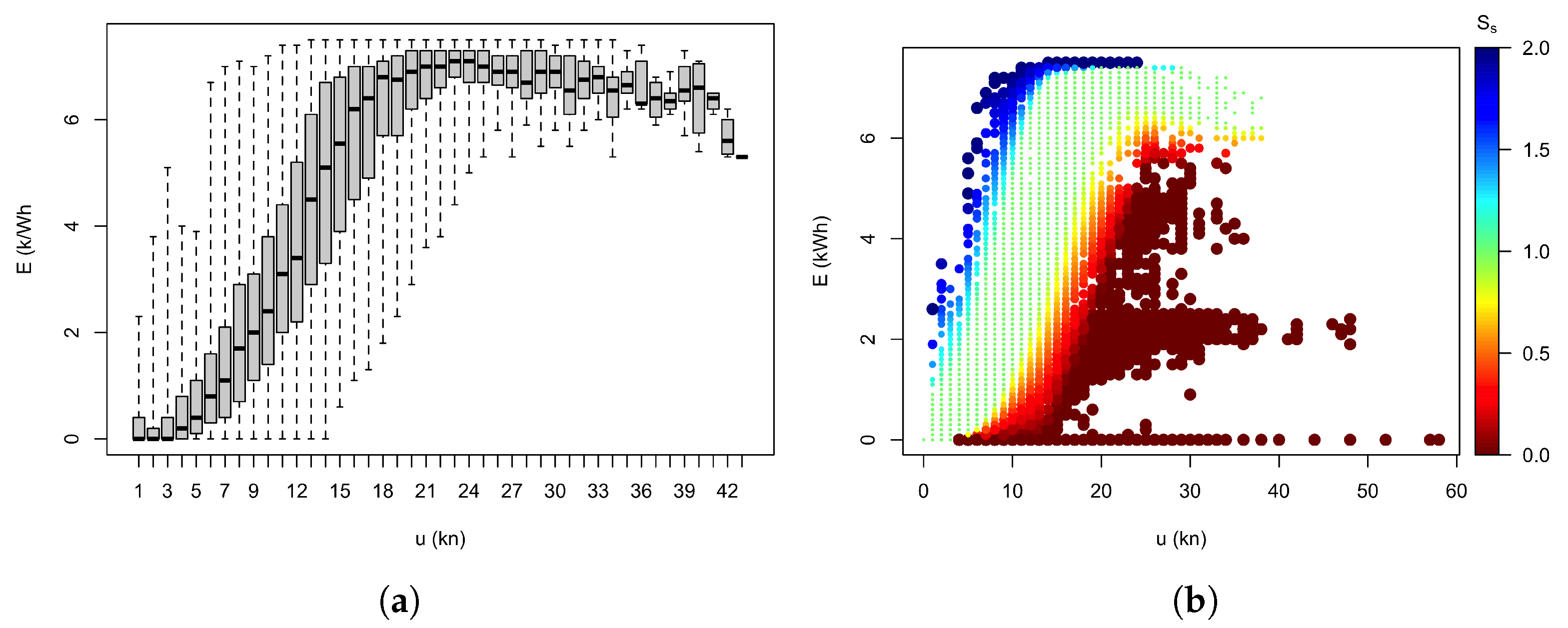
Calculating the quartiles in each wind speed is illustrated by the set of box-and-whisker plots in Figure 3a of electricity production within each wind speed bin of width 1 kn. Production data within the boxes will have a performance score of . Those in the white space below the whiskers will have a score of zero, while those in between are linear interpolations. Likewise, production above the whiskers will have a score of , with those within the upper whiskers will have a score .
Applying the performance indexing of Equation (1) to the validation data and plotting the data from Figure 1b using the performance index to colour-code each measurement clearly demonstrates in Figure 3b the effectiveness of the method in identifying performance outside expected ranges. In particular, the method reliably identifies cases which are recognisably caused by one or more turbines not operating. In addition, it also assigns an index of zero to a range of observations which are below expected but not consistent with a turbine being off-line altogether. They might be cases of below-expectation performance due to other factors such as wear and tear.
Method 1a: Effect of Wind Direction
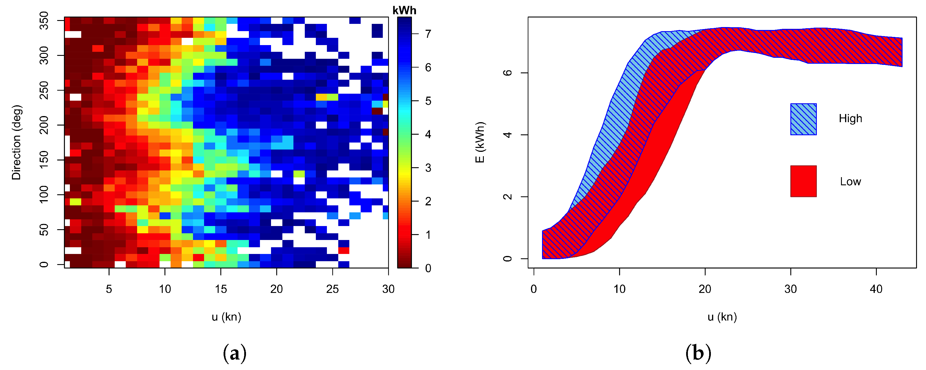
In this section, it is explored to what degree the inclusion of wind direction in the performance index affects its ability to distinguish the different levels of performance. Figure 4a illustrates how strongly the wind direction affects the turbines’ productivity in the form of a heat map of the median productivity of each wind speed–wind direction bin. There is a clear pattern of the installation reaching rated capacity much earlier at wind speeds around 11 kn for wind directions around 70 and 240, and as late as 17 kn around Northerly directions and around 140.
The number of wind speed bins observed in the year’s worth of training data, shown in Figure 2b shows that wind speeds below 2 kn or above 25 kn have less than 100 samples each, preventing meaningful sub-binning into directional bins for calculating . Even for most other wind speeds, the data volume is too small to complete a detailed direction-by-direction analysis. Instead, the two-way separation introduced in Section 2.2.3 was adopted. Within the wind speed range from 2 kn to 25 kn, the samples in each wind speed bin were separated into one subset of all samples with an electricity production above the median within the bin and the other subset of the remaining samples. The wind speed bins outside the 2 to 25 kn range were not subdivided.
Applying this data splitting leads to a clear separation of the boxes and whiskers at intermediate wind speeds. This is illustrated by showing only the interquartile range, i.e. those electricity production values with a performance index , as shaded areas for the two wind speed groups in Figure 4b. Applying these different quartiles to the performance index calculations leads at first sight to a very similar picture to that already seen in Figure 3b. Attempting a more refined directional sensitivity by splitting the data into more groups or by fitting a sinusoidal modulation failed to give any more detail in average performance but actually reduced the distinction between the different subsets. Given this, it was deemed pointless to subdivide the data even further by considering gust information.
3.2. Method 2: PCA
This section presents the results from the purely data-driven method. The potential benefit of this method, in addition to eliminating the need for imposing expected behaviour from standard turbine performance curves, is that it does not suffer from too low a data density in less common wind speeds or directions if the directional information is to be included.
3.2.1. PCA Training
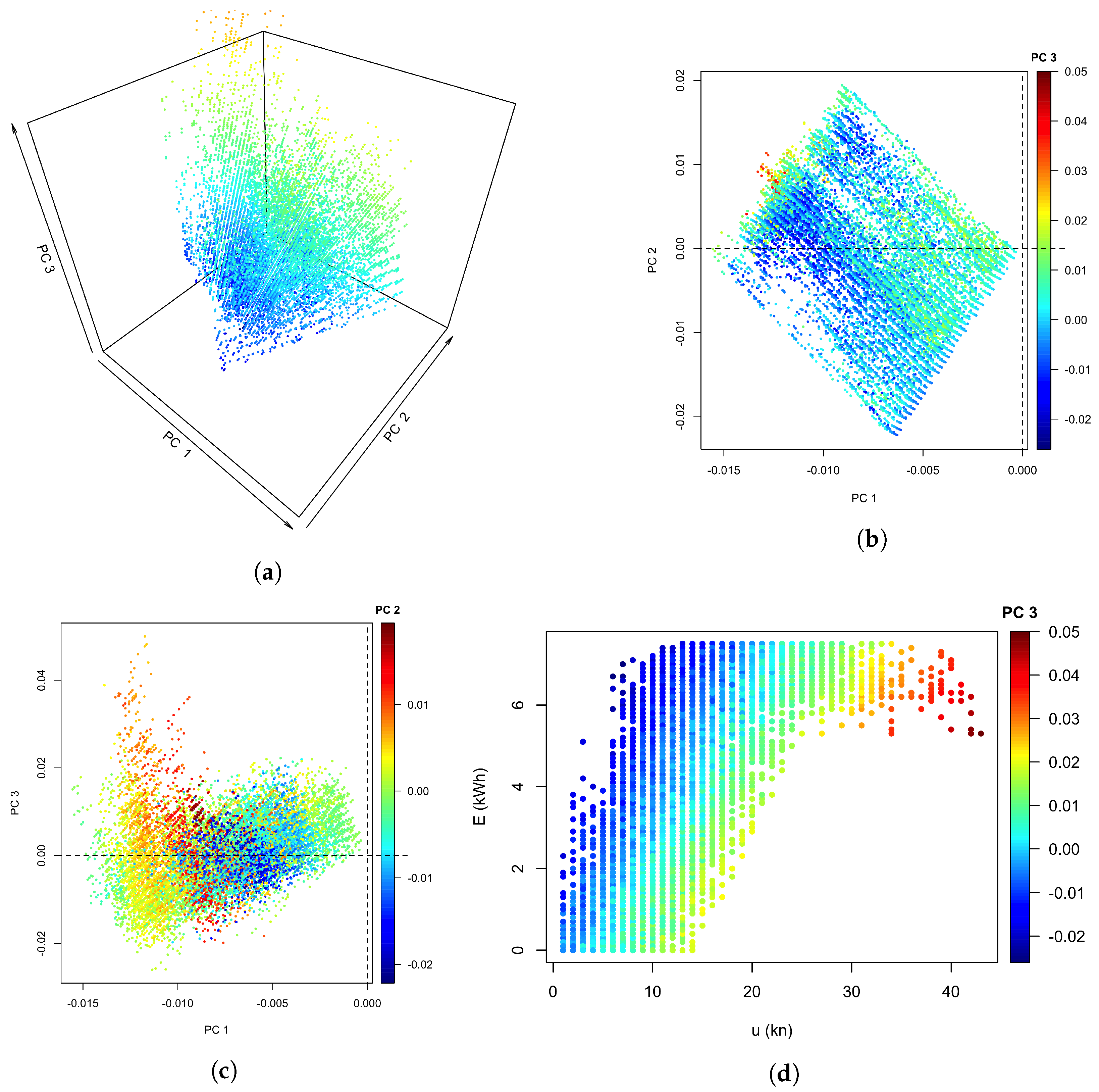
The initial creation of the reference volume representing standard behaviour, applying Equation (2) with electricity production, mean wind speed and its direction, is illustrated in Figure 5, with Figure 5a showing the training data in the 3-dimensional singular vector space, colour-coded by the value of the third principal component. Projections of these data onto planes, with colour-coding by the perpendicular dimension, show that the training data cover an almost rectangular area in the first two directions, in Figure 5b, with the highest value in the third direction near the upper left edge. Looking ’sideways’ along the first and third singular vector in Figure 5c, the projection of the associated principal components results in a curve which is reminiscent of a rotated version of the empirical performance curve from Figure 1a, together with a clear structure in the colour coding by .
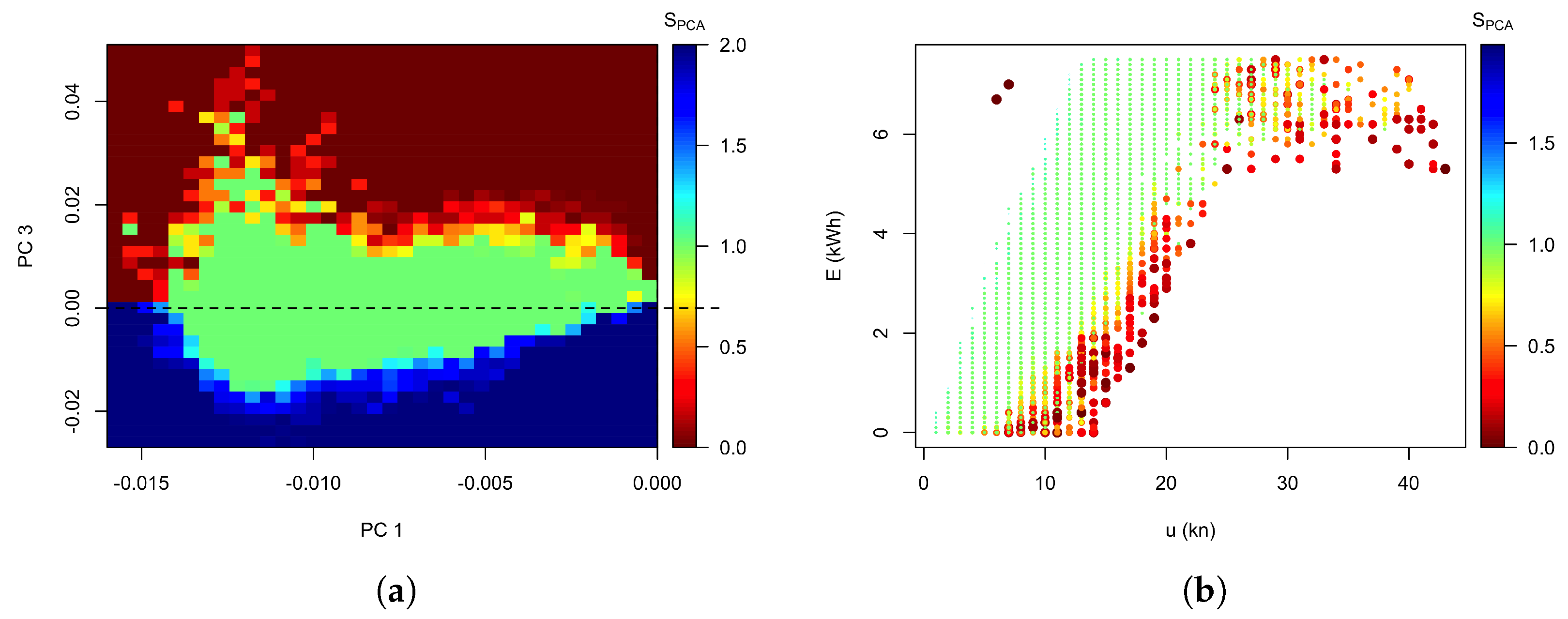
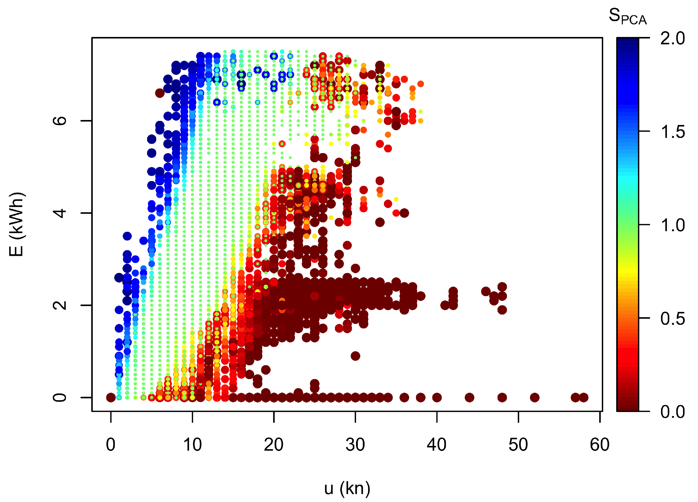
Figure 5d shows a version of Figure 1a but using the value of for the colour scale. This shows that while the first two principal components capture the typical turbine performance curve, the third principal component identifies the turbines’ performance relative to that typical curve, with high values of associated with below-average electricity production and vice versa. Using this insight is used to apply the final correction for the PCA performance curve to distinguish above-expected from below-expected performance by mirroring the initial scores for all points with in Equation (7). The resulting performance score map in the projection is shown in Figure 6a with a colour-coding of deep red indicating unacceptably low productivity, , deep blue exceedingly high productivity, , the central, light green area of ’expected’ behaviour, , and a gradual transition between those main areas.
Calculating the score for each sample from the training data by mapping its associated principal components onto that map results in a performance curve with each sample colour coded according to its PCA performance score, shown in Figure 6a. As seen in Figure 3b, the core of the area has a score of one, and the training data below the core has a score gradually dropping from one to zero at the edge. Above the core, the score increases gradually towards the upper edge of the training data.
3.2.2. Application to the Validation Data Set
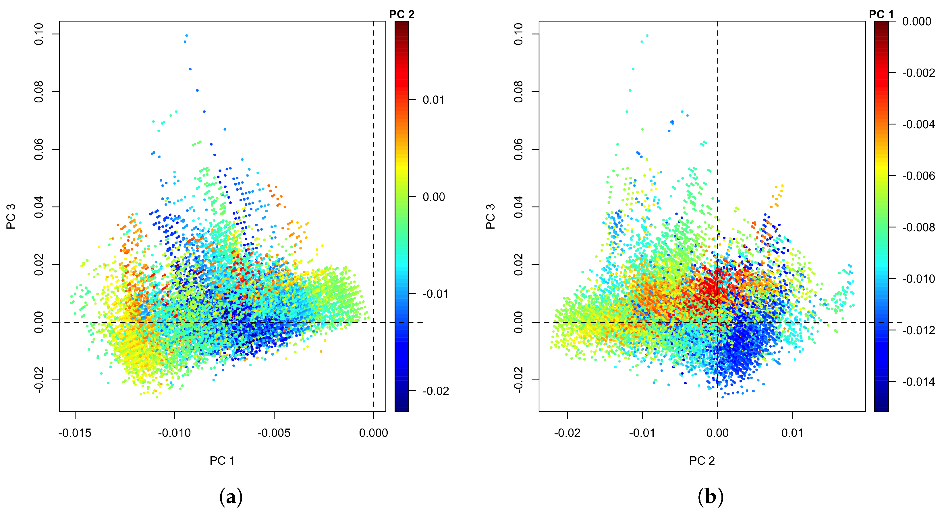
Figure 7 shows the projection of the validation data onto the singular vectors through Equation (3), with the projection equivalent to Figure 5c, onto the - plane in Figure 7a. When comparing this with Figure 5, one observation is that the range of the first and second principal components are about the same in both figures, but the range of the third principal component is increased from an upper limit of 0.05 to 0.1. Some of the additional regions covered form strands extending upwards from the core, similar to the ’hook’ at the left of Figure 5c but placed further right. These strands consist of the three additional horizontal bars corresponding to 0, 1, or 2 turbines operating at their rated capacity and the remaining turbine(s) offline. In addition to those clear features, the core area is also broadened upwards. In this perspective, it is difficult to discern a clear pattern in the value of . The alternative view of the projection onto the - plane in Figure 7b suggests that the value of the first principal component has its maximum mainly in a region of near-zero and slightly positive , while the other extreme is located at slightly positive and negative .
However, since these are projections onto empirically derived orthonormal basis vectors, one should not expect to extract too much obvious information from these graphs without progressing to their use to calculate the performance score. Details aside, the key information communicated by Figure 7 is that validation data from Section 3.1, which are known to contain a significant number of samples with performance well below expected, explore a larger volume in the PCA space than the training data, and that this extended range is primarily found in the higher principal components, most notably here in .
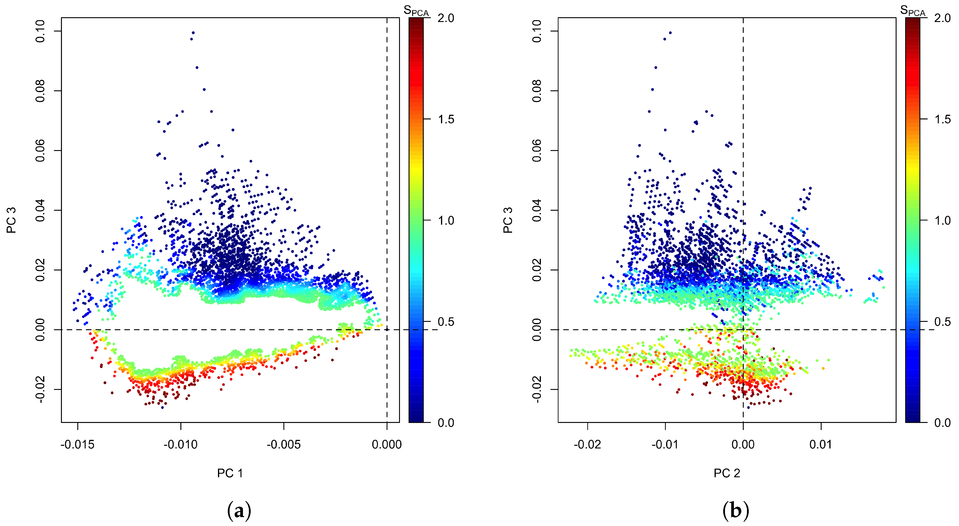
Figure 8 shows the projections of the principal components again, but this time colour-coded with their performance score. To avoid the many samples with a score of that would obscure the other samples, Figure 8 only shows the samples with in green and red, and those with in blue. This shows that all these data are outside the area of in the - projection and either near the extremes of or near the zero point of .
Plotting, as a final step, the conventional performance curve of electricity versus wind speed with each sample colour coded by the performance score calculated in this section, is shown in Figure 9. The main features repeat those that were obtained using the first method with some detailed differences. Since the PCA method is not entirely based on wind speed and electricity production, the visual separation of the scores is not as strict as in Figure 3b with some blue () and some red () examples within the mainly light-green area. The separation between green and blue is more linear here, while it is more reminiscent of a standard turbine performance curve in Figure 3b. Furthermore, the area at moderate wind speeds and low energy productions has more discrimination than Figure 3b, some classified as normal and some as below expectations.
4. Discussion
Given the absence of independently verified performance quality during the second year of operation as well as the absence of a recommended method in the industry or literature other than confirmation of site visits to reset or repair turbines, the critical evaluation of the methods and their usefulness will necessarily rest for the time being mainly on a comparison of the three methods against each other.
4.1. Inter-Model Comparison
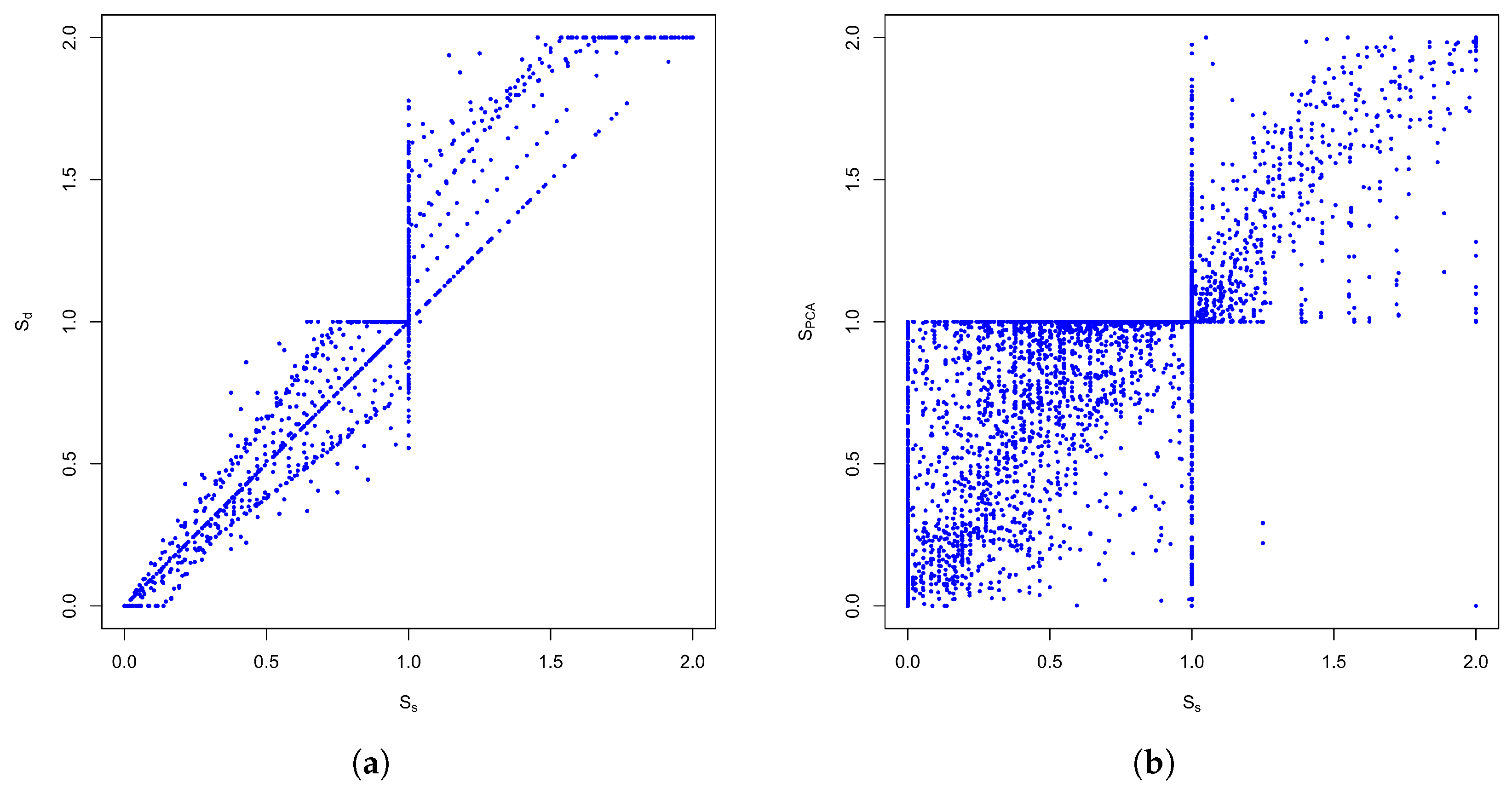
The key differences in the ability to detect sub-optimal performance can be extracted from Figure 10, which shows a scatter plot of the directional performance score in Figure 10a and the PA score, in Figure 10b against , respectively. The diagonal line consists of all points where the performance index from both methods is identical. The vertical line in the middle represents cases where but the other method classed them as outside that interquartile range, and the horizontal line and vice versa. There are almost no instances where one score was above the expected and the other below the expected. One point to notice is that the simple index almost never scored an observation higher than expected when the directional index classed the observation as within expected. In contrast, a number of cases were classed as ’below expectation’ by the simple index when the directional method accepted it as within the expected range. Reversing the perspective, for cases identified as within expected by the simple method, the directional method could go either way. The correlation between the interquartile methods and the PCA method is less clear but still reasonably strong. While the Pearson’s correlation coefficient between and is , it is only around between and either or .
The overall distribution into the main classes using the three methods is summarised in Table 1. While the three methods largely agree, it can be seen that the directional method is the most ’generous,’ awarding high scores and the simple least generous. In contrast, the PCA method has the least instances of zero score and the highest number of . This would indicate that the PCA method might either miss instances where maintenance could improve productivity, but on the other hand, it is less likely to cause false alarms.
4.2. External Validation
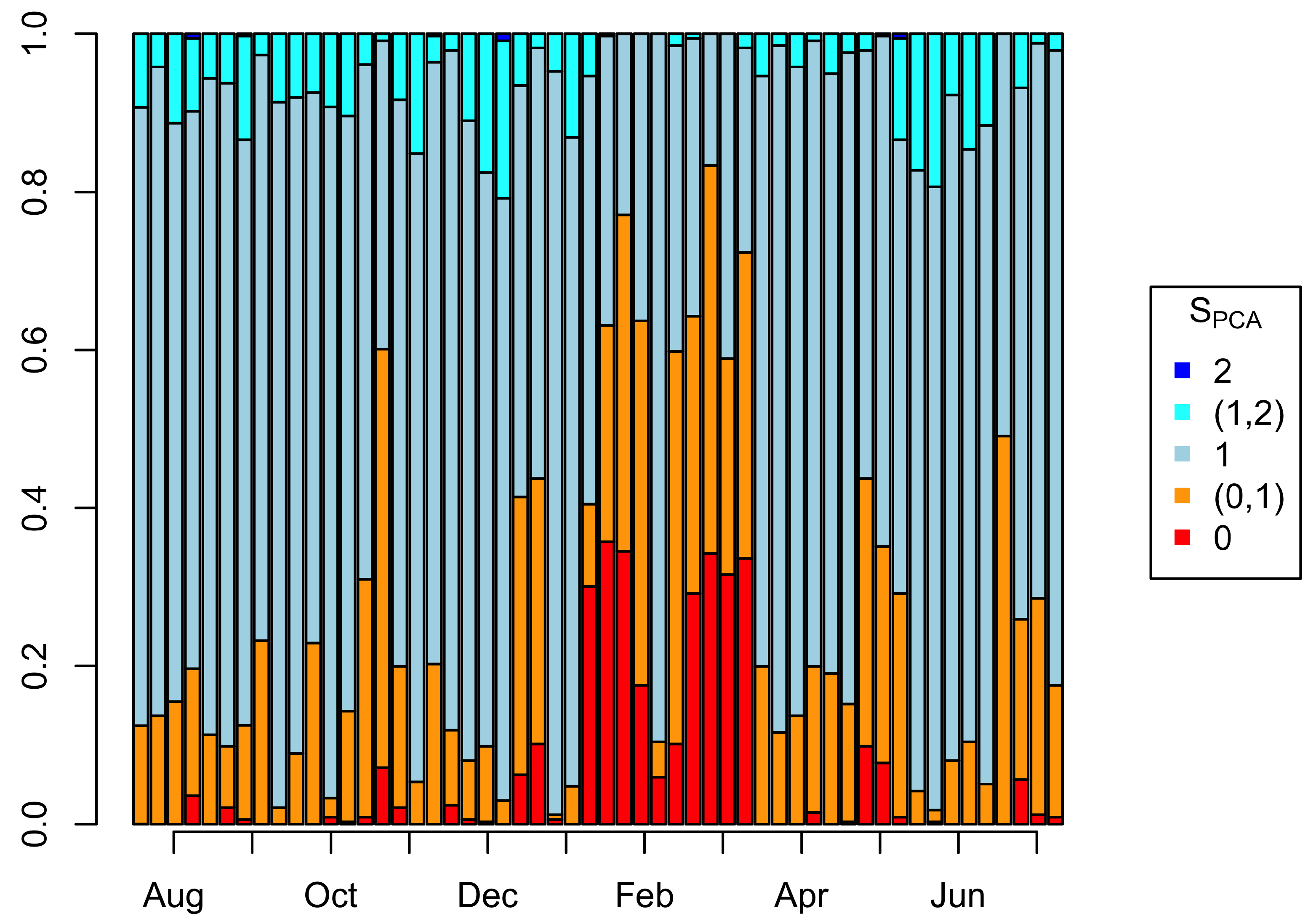
The only external validation available are reports of an engineer visiting the turbines and resetting them when they were down. It is, therefore, instructive to track the performance index over time and compare changes in behaviour against the engineer’s reports. As all three methods are highly correlated, the external validation will be demonstrated against one method only, namely the PCA method. Figure 11 summarises the split of the performance score into the four groups (zero, between zero and 1, 1, between 1 and 2, and 2). The first column gives that split for the entire training period, and each subsequent column shows it within each week of the validation period. The weeks with significantly increased times of , as in October, December, and the period from January to March, May, and July, have been confirmed by the engineer as times with problems with one or more of the turbines. However, in addition to these confirmed events, Figure 11 also shows a gradual increase in samples with below-expected performance. This suggests that the approach is able to identify an underlying gradual trend of increasingly sub-optimal performance due to more subtle causes such as wear and tear.
4.3. Potential Performance Improvement
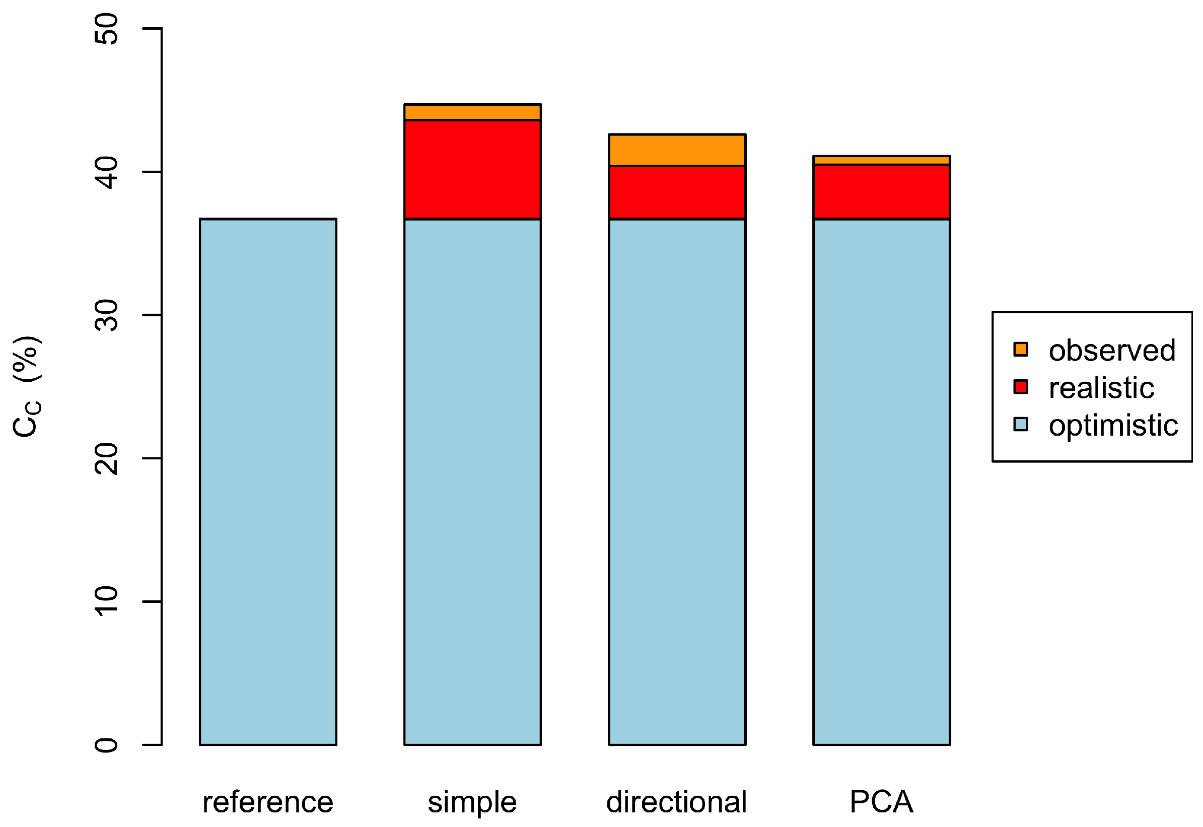
Before addressing future development and validation options, the potential use of the method will be demonstrated in this section. Supposing that this method were consistently used to provide an active maintenance regime targeted to keep the installation’s operation within the expected performance range, it is possible to quantify the potential benefit in terms of additional energy production from the times when the data indicated sub-optimal behaviour. Figure 12 summarises the potential electricity productivity expressed as the capacity factor of the installation. The red area indicates the energy recovered if all instances with were brought up to the average operation within the band of . This can therefore be classed as a realistically achievable improvement.
The orange area on top would be additional electricity operation if the installation could be brought up to the average operation of that observed for all cases with . This means that the maintenance regime would also enable the installation to exceed standard behaviour with the same likelihood as already observed and could therefore be viewed as an upper limit of recoverable electricity. Given that the simple method had the largest number of instances flagged with in Table 1, the expected achievable productivity is highest, while the margin between achievable and upper limit is highest for the directional method. The PCA method, which has been identified as the most cautious method, predicts an achievable improvement similar to that of the directional method and a margin to the upper limit similar to the simple method. Taking this as the most realistic potential, even this improvement from a capacity factor of 36.7% to between 39.8 and 40.5% is substantial, especially as the method does not require additional instrumentation or expensive computing resources.
The analysis presented here has also been applied to ten other turbine installations by the same owner, where the distance between the turbine site and the weather station ranged from 5 to 40 km. The findings from all confirmed the reliability of the method. However, since they all use the same turbine model, are monitored in an identical manner, and are located in the same region of the country, the results are not regarded as a true external validation and, therefore, not presented in detail here. However, the method was able to distinguish poor performance, as measured against the manufacturer’s expected production, due to poor siting from the turbine fault. It was, therefore, able to identify sites which would benefit significantly from a more proactive monitoring protocol and others where additional investment in monitoring or maintenance would be futile.
Since both methods only require metered electricity production and either a regularly monitored weather station within about 40 km or access to hourly wind speed data from databases such as ERA5 [37], the method can be applied to any metered wind turbine anywhere in the world without adaptation. In fact, the ERA5 database includes wind speed, wind direction and gust with global coverage on a quarter-degree grid, providing the ideal reference tool against which to test any wind turbine’s performance.
4.4. Validation and Sensitivity to Training Data
Section 2 acknowledged that some ad-hoc assumptions had to be made to create reliable training data. Given the nature of the available data, this was inevitable. However, the results presented here—identifying clear cases of turbines not working and the overall productivity having gradually reduced over the validation period compared to the training period—is evidence that the method works in principle. Looking forward to applying the method to new installations, there will still be a challenge that it will never be possible to create a gold-standard reference, partly because the scale of these installations prevents the investment into high-resolution anemometers at the turbine sites but also because there is never a guarantee that a reasonable training period would capture the long-term climatology.
One solution to the second problem would be to review the training data periodically in light of new information gathered in the following period. If previously unseen weather conditions are being observed, it will be possible to add those to the training data as long as one is confident that the turbine performance at the same time is consistent with normal operation. Likewise, samples from the original training data set, which are subsequently identified to be unreliable, can be eliminated. The training step to create the reference can then be repeated using the revised training data.
A solution to the first problem is much more challenging. For a complete validation of the methods, one would either have to carry out extensive field trials, continuing the initial work presented in [21], but even that might not provide a firm reference to identify particular types of failures. A validation process suggested here would be to model turbine output based on the manufacturer’s data, to perturb those with typical fluctuations and then to model a specified set of faults. Based on measured wind speed data at a site and a reference site, or using two adjacent grid points from the ERA5 data set, one would then simulate the output from the turbine both, operating normally and with a fault, from one of the wind speed data and correlate that with the other wind speed measurement. This would provide a clear method to train the methods using normally operating turbine simulations and then to identify the signal and resulting performance score from turbines outside their normal operating parameters.
In fact, since no new installation is routinely monitored in detail, such training using simulation would be a standard procedure to train the performance scoring. It would also be a valuable tool in the initial decision-making to estimate a realistic range of expected annual electricity production.
4.5. Development Needs
Before such a validation programme should commence, one further stage in the development of the PCA method should be completed. It has already been mentioned that it would be straightforward—trivial, in fact—to incorporate gust information into the training data. Instead of the input matrix consisting of three column vectors, it would have five column vectors with the additional gust speed and direction. It would also be possible to include wind information at higher levels, for example, at 100 m as is provided by ERA5, temperature and atmospheric pressure, or more than one reference grid point. This has not been presented here as the challenge is how to construct the performance score from a much higher-dimensional PCA space. Presenting this is a significant task which would have obscured the main intention of this paper.
A further refinement of the method could involve the creation of likelihood indicators for scenarios such as a particular number of turbines operating or not by rescaling the training data representing only some of the turbines operating under the observed conditions (in this case, the rescaling would be by and , respectively). From this, the number of turbines could be estimated as a signal to a maintenance engineer.
5. Conclusions
This study has presented the initial development of two alternative methods of monitoring the performance of small wind installations with the minimum of available data. As far as the author is aware, this is the first published attempt to develop such methods in contrast to the extensive literature for large wind turbines and wind farms, which are fully instrumented and monitored through advanced SCADA systems. This minimum requirement consists of only the electricity production at regular time intervals, ideally hourly or half-hourly, and time-aligned wind data either from a weather station in the region or a global database.
While the first method was based on binning data into weather condition bins to create a performance curve aligned with that expected from the manufacturer’s performance data, the second method was entirely data-driven using Principal Component Analysis. Considering that the first method struggled to information beyond the wind speed alone, its future applicability is likely to be limited. In contrast, the PCA method appears to have more potential as it allows multiple reference data to be used. To achieve this potential, the PCA method requires the systematic development and validation work identified in Section 4.
All methods were shown to be able to identify times of problems with the turbines’ operation, both distinct problems such as a turbine going off-line altogether and also a gradual decrease in performance. Given the minimum data and processing requirements, both methods, therefore, have the potential to be viable asset monitoring tools for small installations without the need for additional instrumentation.
Given that the methods were developed and demonstrated against a specific data set, further development and validation against other data sets are needed to build up confidence in the approach. Once the methods are more robustly validated, they can easily be applied to monitor any wind turbine installation anywhere in the world as long as the electricity production is regularly recorded. An initial application to a set of installations has illustrated that the method can distinguish between normal and sub-normal operations, which, if routinely applied, can be used to identify faults quickly and initiate maintenance action. In addition to identifying clear faults, the methods have also identified a gradual decrease in performance which has been attributed to the ageing of the devices.
Supplementary Materials
The following supporting information can be downloaded at: https://www.mdpi.com/article/10.3390/en16083500/s1.
Funding
This research received no external funding.
Data Availability Statement
The data and code (as an R markdown file) are available through Supplementary Material.
Acknowledgments
The author wishes to thank the UK Meteorological Office for providing access to the wind data from the MIDAS record through the CEDA Data Archive (https://archive.ceda.ac.uk/, accessed on 3 February 2023) and for providing the additional anemometer details. We are also extremely grateful to the anonymous provider of the electricity data.
Conflicts of Interest
The author declares no conflict of interest.
Abbreviations
The following key abbreviations and mathematical symbols are used in this manuscript:
| Abbreviations | |
| LCoE | Levelised Cost of Electricity |
| MCP | Measure-Correlate-Predict |
| PCA | Principal Component Analysis |
| SCADA | Supervisory Control and Data Acquisition Software |
| Variables | |
| E | Electricity production in a half-hour period |
| u | Wind speed (in knots) |
| Wind direction (in ) | |
| non-dimensionalised electricity production in a half-hour period | |
| non-dimensionalised wind speed | |
| non-dimensionalised wind direction (in ) | |
| Q | Quartile, with minimum, median, |
| maximum, and the interquartile range between and . | |
| Principal component matrix | |
| Singular value diagonal matrix | |
| Singular vector matrix | |
| Principal component i and column i of | |
| Singular value for | |
| S | Performance Score |
| N | Number of observations in a wind speed bin |
| minimum of for rescaling probability estimate | |
| p | likelihood |
| proxy for likelihood estimator | |
| Subscripts and superscripts | |
| simple performance curve | |
| directionally sub-divided performance curve | |
| PCA based method | |
| indicates interim variables |
References
- Tzen, E. Small wind turbines for on grid and off grid applications. IOP Conf. Ser. Earth Environ. Sci. 2020, 410, 012047. [Google Scholar] [CrossRef]
- Moreira Chagas, C.C.; Pereira, M.G.; Rosa, L.P.; da Silva, N.F.; Vasconcelos Freitas, M.A.; Hunt, J.D. From megawatts to kilowatts: A review of small wind turbine applications, lessons from the US to Brazil. Sustainability 2020, 12, 2760. [Google Scholar] [CrossRef]
- Simic, Z.; Havelka, J.G.; Bozicevic Vrhovcak, M. Small wind turbines—A unique segment of the wind power market. Renew. Energy 2013, 50, 1027–1036. [Google Scholar] [CrossRef]
- Drew, D.R.; Barlow, J.F.; Cockerill, T.T.; Vahdati, M.M. The importance of accurate wind resource assessment for evaluating the economic viability of small wind turbines. Renew. Energy 2015, 77, 493–500. [Google Scholar] [CrossRef]
- Peacock, A.D.; Jenkins, D.; Ahadzi, M.; Berry, A.; Turan, S. Micro wind turbines in the UK domestic sector. Energy Build. 2008, 40, 1324–1333. [Google Scholar] [CrossRef]
- Sunderland, K.M.; Narayana, M.; Putrus, G.; Conlon, M.F.; McDonald, S. The cost of energy associated with micro wind generation: International case studies of rural and urban installations. Energy 2016, 109, 818–829. [Google Scholar] [CrossRef]
- Stehly, T.; Heimiller, D.; Scott, G. Cost of Wind Energy Review; Technical Report; National Renewable Energy Laboratory, US Department of Energy: Golden, CO, USA, 2017. [Google Scholar]
- Bianchini, A.; Bangga, G.; Baring-Gould, I.; Croce, A.; Cruz, J.I.; Damiani, R.; Erfort, G.; Simao Ferreira, C.; Infield, D.; Nayeri, C.N.; et al. Current status and grand challenges for small wind turbine technology. Wind Energy Sci. 2022, 7, 2003–2037. [Google Scholar] [CrossRef]
- Battisti, L.; Benini, E.; Brighenti, A.; Dell’Anna, S.; Raciti Castelli, M. Small wind turbine effectiveness in the urban environment. Renew. Energy 2018, 129, 102–113. [Google Scholar] [CrossRef]
- KC, A.; Whale, J.; Urmee, T. Urban wind conditions and small wind turbines in the built environment: A review. Renew. Energy 2019, 131, 268–283. [Google Scholar] [CrossRef]
- Sunderland, K.; Woolmington, T.; Blackledge, J.; Conlon, M. Small wind turbines in turbulent (urban) environments: A consideration of normal and Weibull distributions for power prediction. J. Wind Eng. Ind. Aerodyn. 2013, 121, 70–81. [Google Scholar] [CrossRef]
- Emejeamara, F.C.; Tomlin, A.S.; Millward-Hopkins, J.T. Urban wind: Characterisation of useful gust and energy capture. Renew. Energy 2015, 81, 162–172. [Google Scholar] [CrossRef]
- Emejeamara, F.C.; Tomlin, A.S. A method for estimating the potential power available to building mounted wind turbines within turbulent urban air flows. Renew. Energy 2020, 153, 787–800. [Google Scholar] [CrossRef]
- Heath, M.; Walshe, J.; Watson, S. Estimating the potential yield of small building-mounted wind turbines. Wind Energy 2007, 10, 271–287. [Google Scholar] [CrossRef]
- Ledo, L.; Kosasih, P.B.; Cooper, P. Roof mounting site analysis for micro-wind turbines. Renew. Energy 2011, 36, 1379–1391. [Google Scholar] [CrossRef]
- Stathopoulos, T.; Alrawashdeh, H.; Al-Quraan, A.; Blocken, B.; Dilimulati, A.; Paraschivoiu, M.; Pilay, P. Urban wind energy: Some views on potential and challenges. J. Wind Eng. Ind. Aerodyn. 2018, 179, 146–157. [Google Scholar] [CrossRef]
- Energy Saving Trust. Location, Location, Location: Domestic Small-Scale Wind Field Trial Report; Technical Report; Energy Saving Trust: London, UK, 2007. [Google Scholar]
- García Márquez, F.P.; Tobias, A.M.; Pinar Pérez, J.M.; Papaelias, M. Condition monitoring of wind turbines: Techniques and methods. Renew. Energy 2012, 46, 169–178. [Google Scholar] [CrossRef]
- Gonzalez, E.; Stephen, B.; Infield, D.; Melero, J.J. Using high-frequency SCADA data for wind turbine performance monitoring: A sensitivity study. Renew. Energy 2019, 131, 841–853. [Google Scholar] [CrossRef]
- Kong, K.; Dyer, K.; Payne, C.; Hamerton, I.; Weaver, P.M. Progress and Trends in Damage Detection Methods, Maintenance, and Data-driven Monitoring of Wind Turbine Blades—A Review. Renew. Energy Focus 2022, 44, 390–412. [Google Scholar] [CrossRef]
- Sissons, M.F.; James, P.A.; Bradford, J.; Myers, L.E.; Bahaj, A.S.; Anwar, A.; Green, S. Pole-mounted horizontal axis micro-wind turbines: UK field trial findings and market size assessment. Energy Policy 2011, 39, 3822–3831. [Google Scholar] [CrossRef]
- Damanik, N.; Robiansyah, M.R.; Apriliana, A.; Purba, S. Design of Energy Monitoring System for Small Scale Wind Turbine Applications. IOP Conf. Ser. Earth Environ. Sci. 2019, 345, 012003. [Google Scholar] [CrossRef]
- Lydia, M.; Kumar, S.S.; Selvakumar, A.I.; Prem Kumar, G.E. A comprehensive review on wind turbine power curve modeling techniques. Renew. Sustain. Energy Rev. 2014, 30, 452–460. [Google Scholar] [CrossRef]
- Creech, A.; Früh, W.G.; Maguire, A.E. Simulations of an Offshore Wind Farm Using Large-Eddy Simulation and a Torque-Controlled Actuator Disc Model. Surv. Geophys. 2015, 36, 1–55. [Google Scholar] [CrossRef]
- Bulaevskaya, V.; Wharton, S.; Clifton, A.; Qualley, G.; Miller, W.O. Wind power curve modeling in complex terrain using statistical models. J. Renew. Sustain. Energy 2015, 7, 013103. [Google Scholar] [CrossRef]
- Ouyang, T.; Kusiak, A.; He, Y. Modeling wind-turbine power curve: A data partitioning and mining approach. Renew. Energy 2017, 102, 1–8. [Google Scholar] [CrossRef]
- Marvuglia, A.; Messineo, A. Monitoring of wind farms’ power curves using machine learning techniques. Appl. Energy 2012, 98, 574–583. [Google Scholar] [CrossRef]
- Stephen, B.; Galloway, S.J.; McMillan, D.; Hill, D.C.; Infield, D.G. A copula model of wind turbine performance. IEEE Trans. Power Syst. 2011, 26, 965–966. [Google Scholar] [CrossRef]
- Jollife, I.T.; Cadima, J. Principal component analysis: A review and recent developments. Philos. Trans. R. Soc. A Math. Phys. Eng. Sci. 2016, 374, 20150202. [Google Scholar] [CrossRef]
- Jolliffe, I.T. Principal Component Analysis, 2nd ed.; Springer: New York, NY, USA, 2002. [Google Scholar] [CrossRef]
- Skittides, C.; Früh, W.G. Wind forecasting using Principal Component Analysis. Renew. Energy 2014, 69, 365–374. [Google Scholar] [CrossRef]
- Zakaria, A.; Früh, W.G.; Ismail, F.B. Wind resource forecasting using enhanced measure correlate predict (MCP). AIP Conf. Proc. 2018, 2035, 040005. [Google Scholar] [CrossRef]
- Broomhead, D.S.; Jones, R.; King, G.P.; Pike, E.R. Singular systems. In Chaos, Noise and Fractals, 1st ed.; Pike, E.R., Lugiato, L.A., Eds.; Adam Hilger: Bristol, UK, 1987; pp. 15–27. [Google Scholar]
- Skittides, C.; Früh, W.G. A new Measure-Correlate-Predict Wind Resource Prediction method. In Proceedings of the International Conference on Renewable Energies and Power Quality (ICREPQ’15), La Coruña, Spain, 25–27 April 2015; Volume 13, pp. 612–615. [Google Scholar] [CrossRef]
- Früh, W.G. From local wind energy resource to national wind power production. AIMS Energy 2015, 3, 101–120. [Google Scholar] [CrossRef]
- UK Meteorological Office. Met Office Integrated Data Archive System (MIDAS) Land and Marine Surface Stations Data (1853–Current); NCAS British Atmospheric Data Centre: Oxford, UK, 2012; Available online: https://archive.ceda.ac.uk/ (accessed on 3 February 2023).
- Copernicus Climate Change Service, Climate Data Store. ERA5 Hourly Data on Single Levels from 1940 to Present. 2023. Available online: https://cds.climate.copernicus.eu/cdsapp#!/dataset/reanalysis-era5-single-levels (accessed on 10 April 2023).
Figure 1.
Scatter plot of electricity production against wind speed at a distance of 25 km, (a) Training data for the training period, and (b) Validation data for the validation period.
Figure 1.
Scatter plot of electricity production against wind speed at a distance of 25 km, (a) Training data for the training period, and (b) Validation data for the validation period.

Figure 2.
Wind climate during the training period, with (a) the wind rose at the anemometer site and (b) the number of samples observed in each wind speed bin (wind speeds in knots) together with the best-fit Weibull curve (red line). The horizontal dashed line indicates 1% of the total number of samples.

Figure 3.
(a) Empirical performance curve as a set of boxplots for each wind speed bin from the training data; (b) scatter plot of the validation data, with colour coding for the performance score, , for each sample.
Figure 3.
(a) Empirical performance curve as a set of boxplots for each wind speed bin from the training data; (b) scatter plot of the validation data, with colour coding for the performance score, , for each sample.

Figure 4.
(a) Heat map of the median electricity production by wind speed and direction. (b) Refinement of performance expectations for distinct wind directions, showing the bands of for the two directional subsets.
Figure 4.
(a) Heat map of the median electricity production by wind speed and direction. (b) Refinement of performance expectations for distinct wind directions, showing the bands of for the two directional subsets.

Figure 5.
Principal components from training data: (a) 3D scatter plot, (b) projection onto the - plane with points colour-coded by , (c) projection onto the - plane colour-coded by , (d) empirical performance curve colour-coded by .
Figure 5.
Principal components from training data: (a) 3D scatter plot, (b) projection onto the - plane with points colour-coded by , (c) projection onto the - plane colour-coded by , (d) empirical performance curve colour-coded by .

Figure 6.
PCA score, , (a) score map in - projection, and (b) empirical performance curve for the training data colour-coded by .
Figure 6.
PCA score, , (a) score map in - projection, and (b) empirical performance curve for the training data colour-coded by .

Figure 7.
(a) Principal components against for the validation data, colour-coded by ; (b) the same but against colour-coded by .
Figure 7.
(a) Principal components against for the validation data, colour-coded by ; (b) the same but against colour-coded by .

Figure 8.
Principal components of subset of validation data with a performance score ; (a) against , (b) against .
Figure 8.
Principal components of subset of validation data with a performance score ; (a) against , (b) against .

Figure 9.
Performance curve for the validation period with colour coding for .

Figure 10.
Scatter plot of performance index from two methods, (a) directional score, against the simple score , and (b) PCA score against .
Figure 10.
Scatter plot of performance index from two methods, (a) directional score, against the simple score , and (b) PCA score against .

Figure 11.
Weekly distribution of the performance index over time for the validation data, with the initial column the total distribution for the training data.
Figure 11.
Weekly distribution of the performance index over time for the validation data, with the initial column the total distribution for the training data.

Figure 12.
Potential improvement in annual productivity shown as the observed and potentially increased capacity factor, where the actual output is the blue bar, the red section the additional production which should be achievable with responsive maintenance, and the orange section an optimistic high expectation of the yield.


Table 1.
Summary of performance identification. Number given in percent of total sample size of 17,894.
Table 1.
Summary of performance identification. Number given in percent of total sample size of 17,894.
| Method | |||||
|---|---|---|---|---|---|
| simple | 14.3 | 29.6 | 51.1 | 4.6 | 0.5 |
| directional | 15.3 | 20.9 | 52.7 | 10.0 | 1.1 |
| PCA | 5.9 | 27.1 | 58.7 | 8.2 | 0.0 |
Disclaimer/Publisher’s Note: The statements, opinions and data contained in all publications are solely those of the individual author(s) and contributor(s) and not of MDPI and/or the editor(s). MDPI and/or the editor(s) disclaim responsibility for any injury to people or property resulting from any ideas, methods, instructions or products referred to in the content. |
© 2023 by the author. Licensee MDPI, Basel, Switzerland. This article is an open access article distributed under the terms and conditions of the Creative Commons Attribution (CC BY) license (https://creativecommons.org/licenses/by/4.0/).
Share and Cite
MDPI and ACS Style
Früh, W.-G. Assessing the Performance of Small Wind Energy Systems Using Regional Weather Data. Energies 2023, 16, 3500. https://doi.org/10.3390/en16083500
AMA Style
Früh W-G. Assessing the Performance of Small Wind Energy Systems Using Regional Weather Data. Energies. 2023; 16(8):3500. https://doi.org/10.3390/en16083500
Chicago/Turabian StyleFrüh, Wolf-Gerrit. 2023. "Assessing the Performance of Small Wind Energy Systems Using Regional Weather Data" Energies 16, no. 8: 3500. https://doi.org/10.3390/en16083500
Note that from the first issue of 2016, this journal uses article numbers instead of page numbers. See further details here.