
Non-Intrusive Voltage-Inversion Measurement Method for Overhead Transmission Lines Based on Near-End Electric-Field Integration

Abstract
:1. Introduction
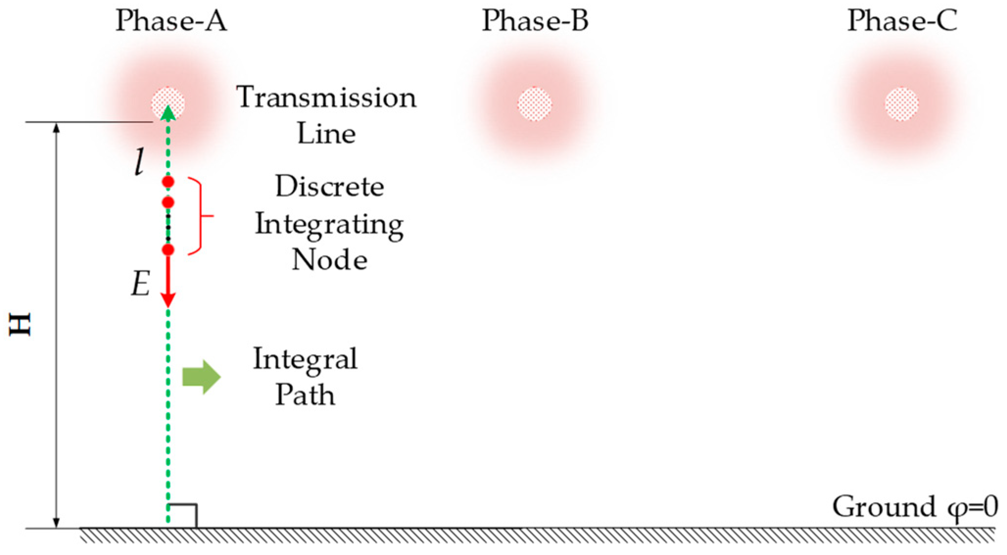
2. The Measurement Principle of the Near-End Electric-Field Integral Method
2.1. Electric-Field Integration Method
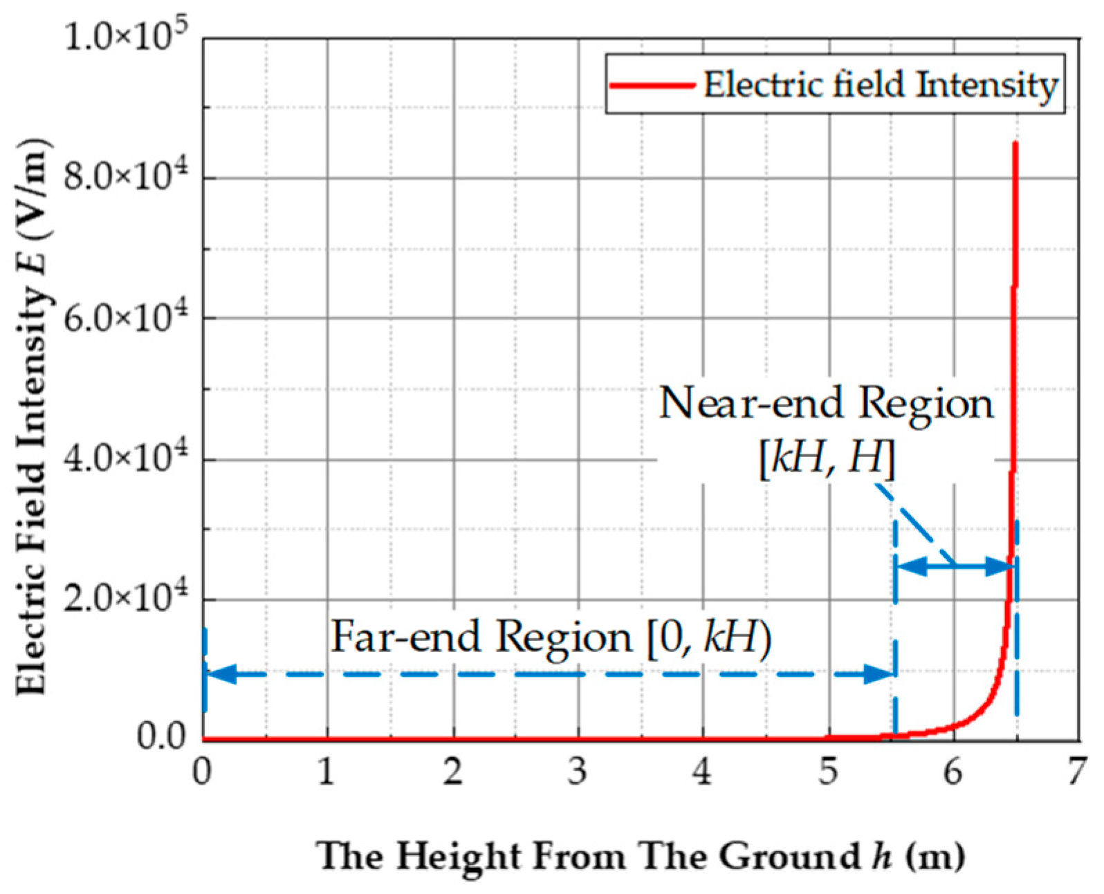
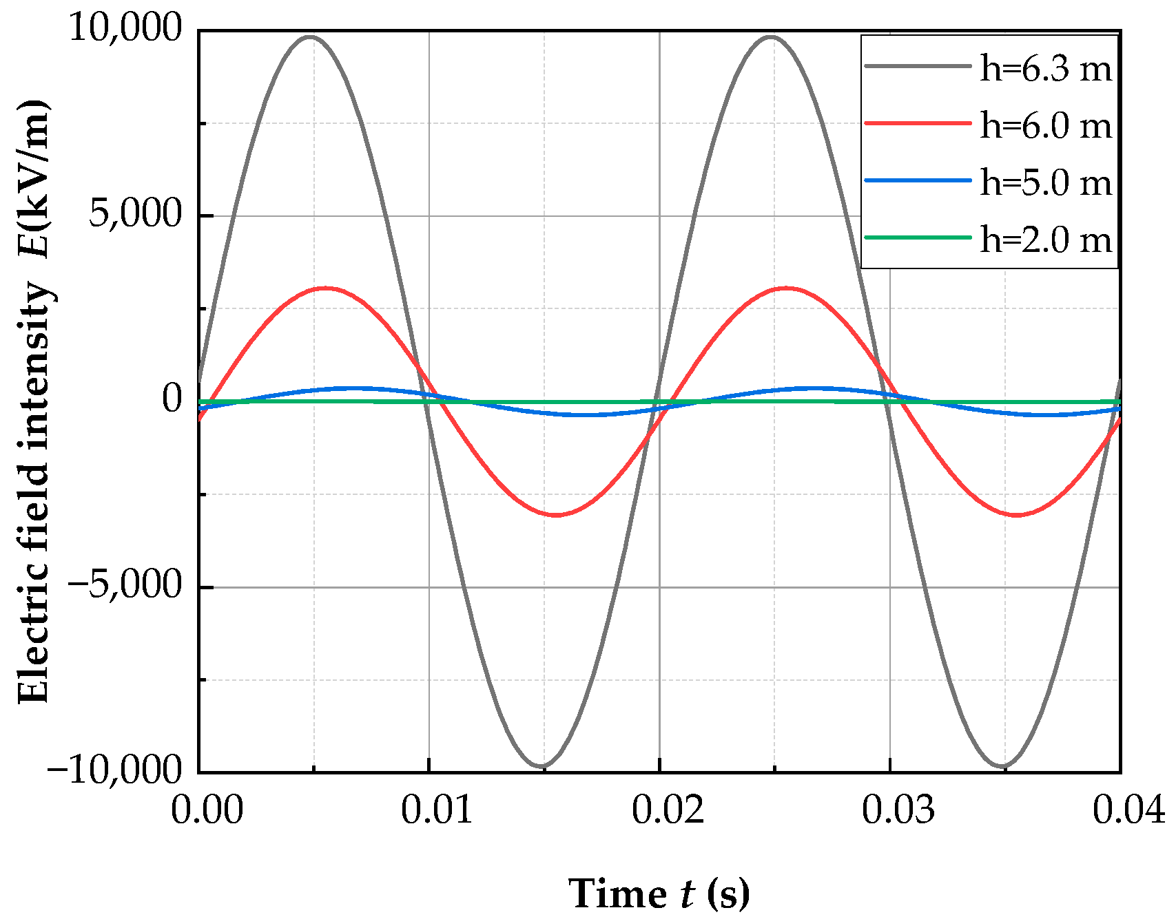
2.2. Analysis of Electric-Field Distribution of Plumb Line below the Line
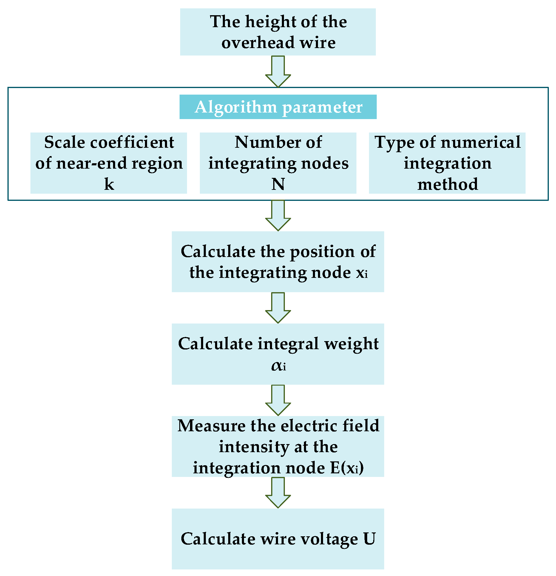
2.3. The Principle of the Near-End Electric-Field Integral Method
- (1)
- Gauss–Legendre integral
- (2)
- Gauss–Chebyshev integral
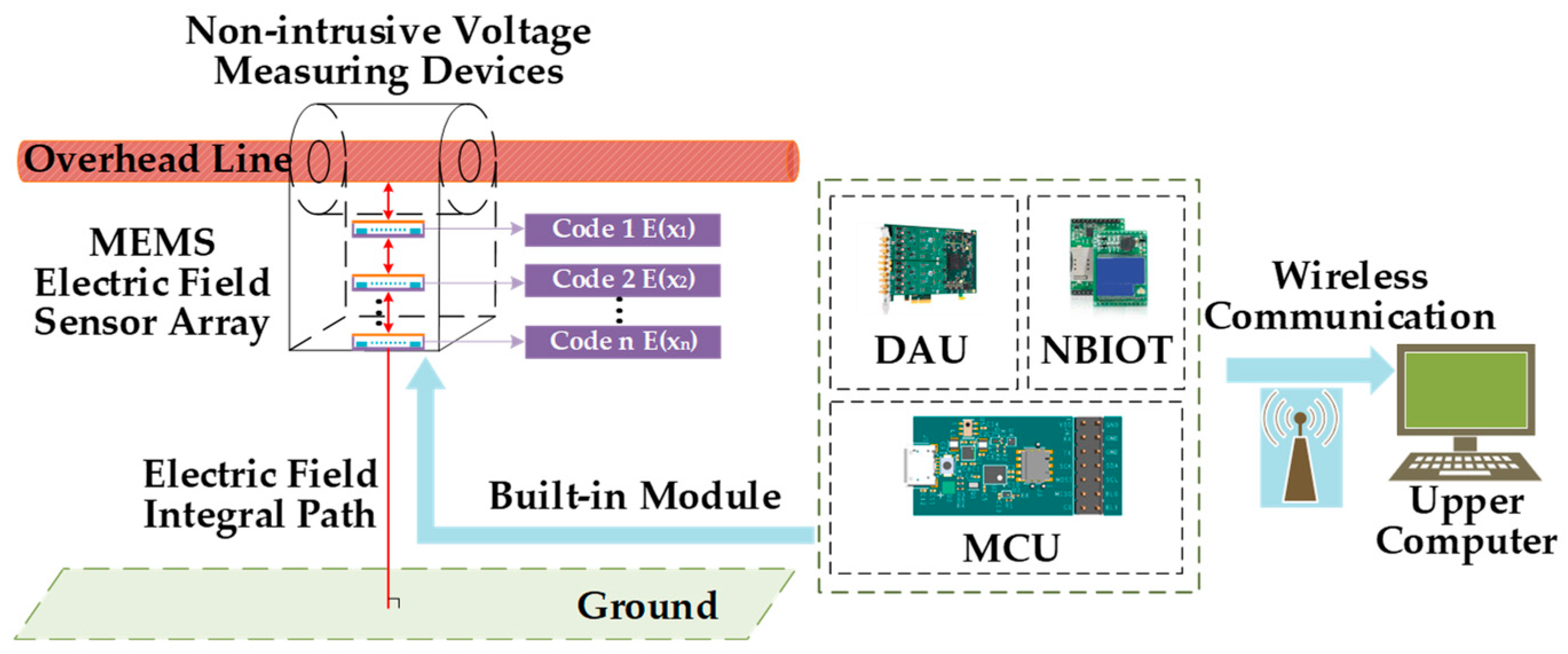
2.4. Scheme of the Measurement System
3. Optimization of Near-End Electric-Field Integration Algorithm
3.1. Numerical Integration Type and Node Number Optimization
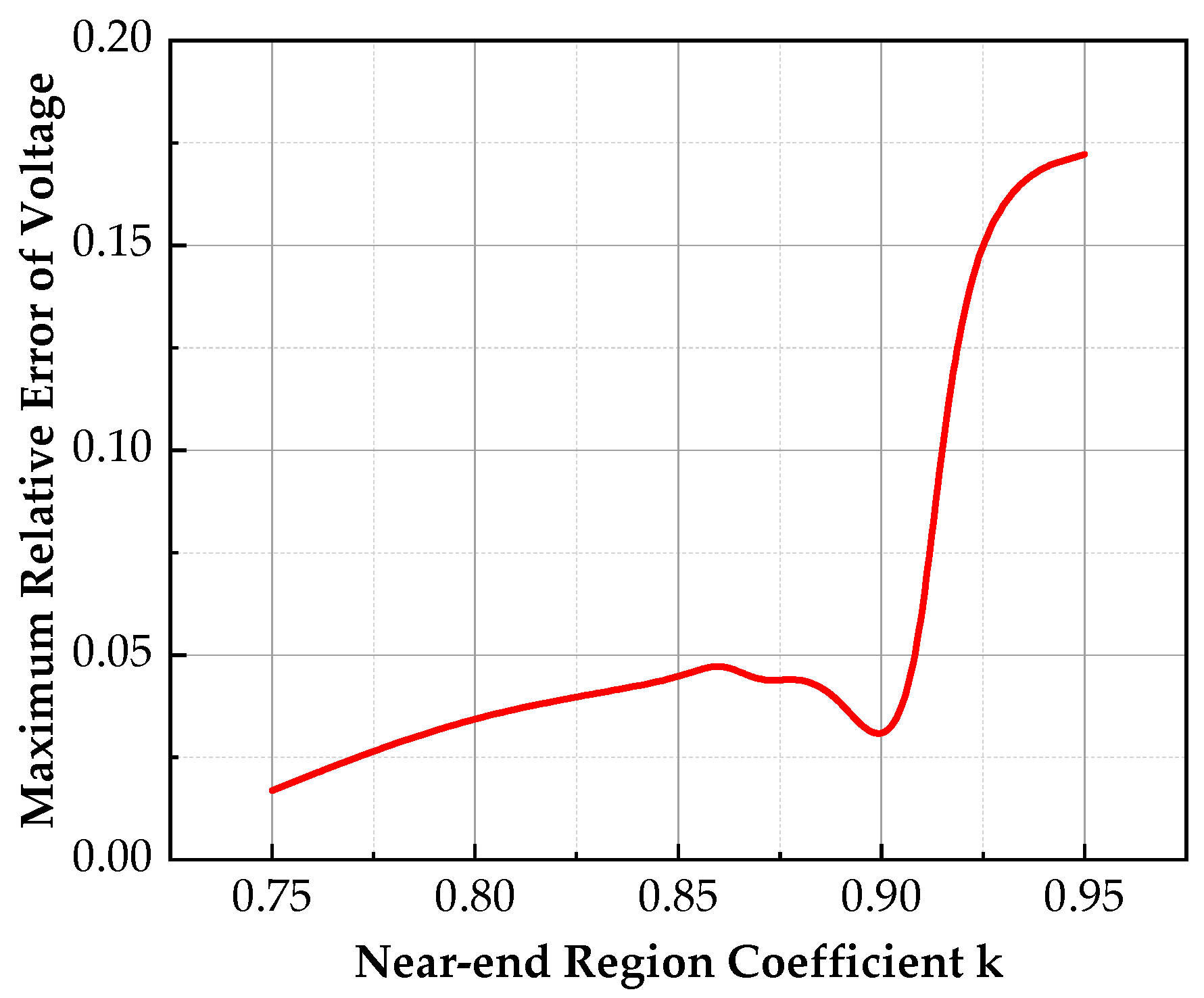
3.2. Optimization of the Near-End Region Coefficient k
4. Experimental Testing and Analysis
4.1. Construction of Experimental Platform
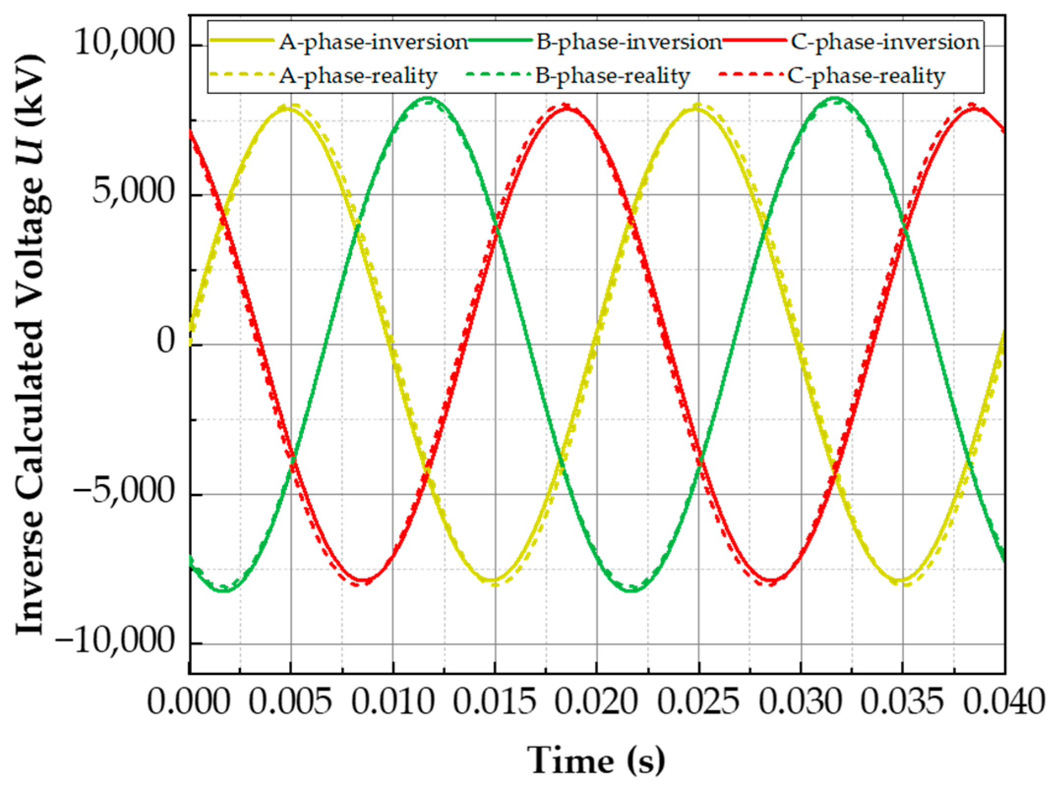
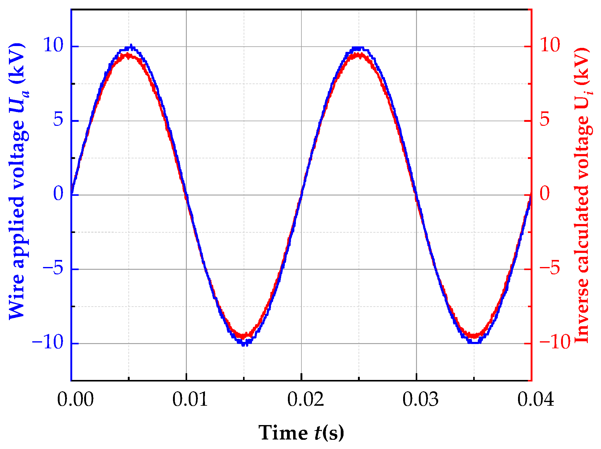
4.2. Analysis of Experimental Results
5. Conclusions
- (1)
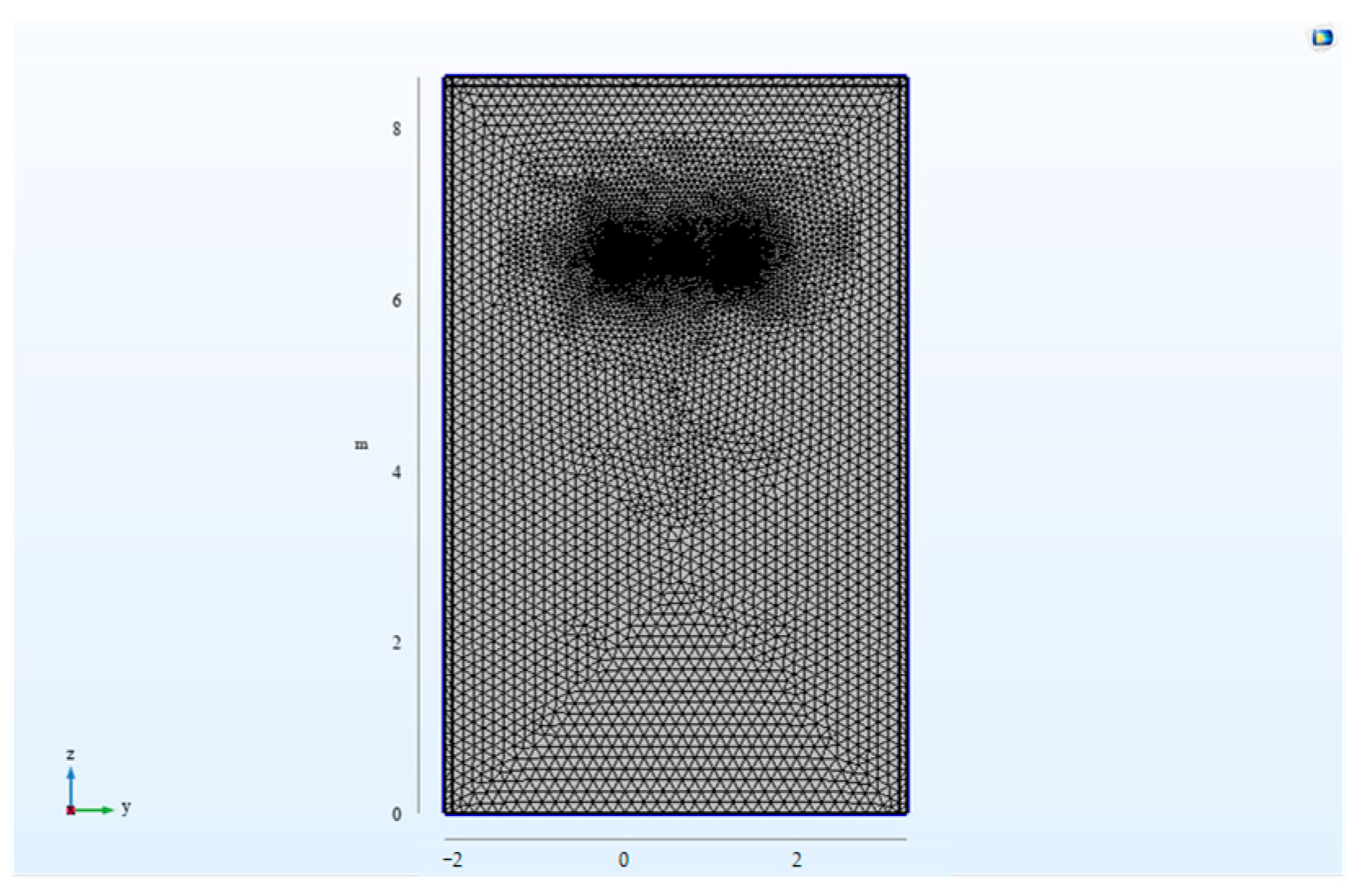
- The theoretical model of voltage inversion calculated by the electric-field integral method is established. The COMSOL Multiphysics finite element simulation software is employed to calculate the electric-field distribution under the 10 kV three-phase overhead line and the electric-field intensity waveform at different positions. The calculation results indicate that the electric-field intensity on the plumb line below the conductor is concentrated in the near-end region of the conductor, and the integration node in the near-end region is less affected by the electric-field crosstalk of the adjacent phase conductor. Then, a voltage-inversion algorithm based on the near-end electric-field integration method is proposed in this paper. Meanwhile, an overhead-line-voltage monitoring system is proposed based on the near-end electric-field integration method.
- (2)
- The voltage-inversion calculation is conducted by using the data of a finite simulated electric field, and the integration type, the number of integration nodes, the proportion coefficient of the proximal integration region, and the remote auxiliary nodes of the voltage-inversion algorithm are optimized. The results indicate that when k = 0.9, the three-point Gauss–Chebyshev integral method can realize accurate inversion of three-phase voltage, and the maximum error is 2.55%.
- (3)
- A test platform is built for voltage-inversion measurement of high-voltage overhead lines, and the electric-field waveform at each integral node below the line is measured through the MEMS electric-field sensor. The results indicate that when the ratio coefficient of the proximal region is k = 0.7, the error of voltage inversion by using the three-point Gauss–Chebyshev integral method and introducing a remote auxiliary node is 5.75%.
Author Contributions
Funding
Data Availability Statement
Conflicts of Interest
References
- Strasser, T.; Andren, F.; Kathan, J.; Cecati, C.; Buccella, C.; Siano, P.; Leitao, P.; Zhabelova, G.; Vyatkin, V.; Vrba, P.; et al. A review of architectures and concepts for intelligence in future electric energy systems. IEEE Trans. Ind. Electron. 2015, 62, 2424–2438. [Google Scholar] [CrossRef] [Green Version]
- Huang, A.Q.; Crow, M.L.; Heydt, G.T.; Zheng, J.P.; Dale, S.J. The future renewable electric energy delivery and management (FREEDM) system: The energy internet. Proc. IEEE 2010, 99, 133–148. [Google Scholar] [CrossRef]
- Morello, R.; Mukhopadhyay, S.C.; Liu, Z.; Slomovitz, D.; Samantaray, S.R. Advances on sensing technologies for smart cities and power grids: A review. IEEE Sens. J. 2017, 17, 7596–7610. [Google Scholar] [CrossRef]
- De La Cruz, J.; Gómez-Luna, E.; Ali, M.; Vasquez, J.C.; Guerrero, J.M. Fault location for distribution smart grids: Literature overview, challenges, solutions, and future trends. Energies 2023, 16, 2280. [Google Scholar] [CrossRef]
- Zhang, W.; Yang, Y.; Zhao, J.; Huang, R.; Cheng, K.; He, M. Research on a non-contact multi-electrode voltage sensor and signal processing algorithm. Sensors 2022, 22, 8573. [Google Scholar] [CrossRef] [PubMed]
- Zhang, W.; Wei, R.; Jiu, A.; Cheng, K.; Yang, Y.; Suo, C. Self-Calibration Method of Noncontact AC Voltage Measurement. Electronics 2023, 12, 300. [Google Scholar] [CrossRef]
- Shenil, P.S.; George, B. Nonintrusive ac voltage measurement unit utilizing the capacitive coupling to the power system ground. IEEE Trans. Instrum. Meas. 2021, 70, 1–8. [Google Scholar] [CrossRef]
- Xue, F.; Hu, J.; Guo, Y.; Han, G.; Ouyang, Y.; Wang, S.X.; He, J. Piezoelectric–piezoresistive coupling mems sensors for measurement of electric fields of broad bandwidth and large dynamic range. IEEE Trans. Ind. Electron. 2020, 67, 551–559. [Google Scholar] [CrossRef]
- Li, J.; Liu, J.; Peng, C.; Liu, X.; Wu, Z.; Zheng, F. Design and Testing of a Non-Contact MEMS Voltage Sensor Based on Single-Crystal Silicon Piezoresistive Effect. Micromachines 2022, 13, 619. [Google Scholar] [CrossRef]
- Luo, M.; Yang, Q.; Dong, F.; Chen, N.; Liao, W. Miniature micro-ring resonator sensor with electro-optic polymer cladding for wide-band electric field measurement. J. Light. Technol. 2022, 40, 2577–2584. [Google Scholar] [CrossRef]
- Yang, Q.; Sun, S.; He, Y.; Han, R. Intense electric-field optical sensor for broad temperature-range applications based on a piecewise transfer function. IEEE Trans. Ind. Electron. 2019, 66, 1648–1656. [Google Scholar] [CrossRef]
- Wang, J.; Gao, C.; Yang, J. Design, Experiments and Simulation of Voltage Transformers on the Basis of a Differential Input D-dot Sensor. Sensors 2014, 14, 12771–12783. [Google Scholar] [CrossRef] [Green Version]
- Metwally, I.A. D-dot probe for fast-front high-voltage measurement. IEEE Trans. Instrum. Meas. 2010, 59, 2211–2219. [Google Scholar] [CrossRef]
- Yang, P.; Wen, X.; Chu, Z.; Ni, X.; Peng, C. Non-intrusive DC voltage measurement based on resonant electric field microsensors. J. Micromech. Microeng. 2021, 31, 064001. [Google Scholar] [CrossRef]
- Yang, P.; Wen, X.; Lv, Y.; Chu, Z.; Peng, C. A non-intrusive voltage measurement scheme based on MEMS electric field sensors: Theoretical analysis and experimental verification of AC power lines. Rev. Sci. Instrum. 2021, 92, 065002. [Google Scholar] [CrossRef]
- Haberman, M.A.; Spinelli, E.M. A noncontact voltage measurement system for power-line voltage waveforms. IEEE Trans. Instrum. Meas. 2020, 69, 2790–2797. [Google Scholar] [CrossRef]
- Sevlian, R.A.; Rajagopal, R. Actively calibrated line mountable capacitive voltage transducer for power systems applications. IEEE Trans. Smart Grid 2018, 9, 3942–3953. [Google Scholar] [CrossRef] [Green Version]
- Han, Z.; Xue, F.; Hu, J.; He, J. Micro electric field sensors: Principles and applications. IEEE Trans. Ind. Electron. 2021, 15, 35–42. [Google Scholar] [CrossRef]
- Kainz, A.; Steiner, H.; Schalko, J.; Jachimowicz, A.; Kohl, F.; Stifter, M.; Beigelbeck, R.; Keplinger, F.; Hortschitz, W. Distortion-free measurement of electric field strength with a MEMS sensor. Nat. Electron. 2018, 1, 68–73. [Google Scholar] [CrossRef] [PubMed]
- Hu, G.; Li, P.; Liu, X.; Zhao, Y. Inverse source problems in electrodynamics. Inverse Probl. Imaging 2018, 12, 1411–1428. [Google Scholar] [CrossRef] [Green Version]
- Xiao, D.; Xie, Y.; Liu, H.; Ma, Q.; Zheng, Q.; Zhan, Z. Position optimization of measuring points in voltage noncontact measurement of ac overhead transmission lines. Appl. Comput. Electrom. 2017, 32, 908–914. [Google Scholar]
- Chavez, P.P.; Rahmatian, F.; Jaeger, N. Accurate voltage measurement with electric field sampling using permittivity-shielding. IEEE Trans. Power Deliv. 2002, 17, 362–368. [Google Scholar] [CrossRef]
- Rahmatian, F.; Chavez, P.P.; Jaeger, N. 230 kV optical voltage transducers using multiple electric field sensors. IEEE Trans. Power Deliv. 2002, 17, 417–422. [Google Scholar] [CrossRef]
- Chavez, P.P.; Jaeger, N.A.F.; Rahmatian, F. Accurate voltage measurement by the quadrature method. IEEE Trans. Power Deliv. 2003, 18, 14–19. [Google Scholar] [CrossRef]
- Wang, J.; Li, X.; Wang, Q.; Zhong, L.; Zhu, X. Research on transmission line voltage measurement method based on Gauss-Kronrod integral algorithm. Meas. Sci. Technol. 2020, 31, 85103. [Google Scholar] [CrossRef]
- Wang, J.; Yan, X.; Li, X.; Liao, J.; Tao, Y. Method and experimental study of transmission line voltage measurement based on a gauss-type integral algorithm. Trans. China Electrotech. Soc. 2021, 36, 3978–3986. (In Chinese) [Google Scholar]
- Wen, X.; Yang, P.; Chu, Z.; Peng, C.; Liu, Y.; Wu, S. Toward Atmospheric Electricity Research: A Low-Cost, Highly Sensitive and Robust Balloon-Borne Electric Field Sounding Sensor. IEEE Sens. J. 2021, 21, 13405–13416. [Google Scholar] [CrossRef]


| Integral Method | The Number of Integration Nodes N | εr-A | εr-B | εr-C |
|---|---|---|---|---|
| Gauss–Legendre Integral | 2 | −43.21% | −41.33% | −43.47% |
| 3 | −37.17% | −34.10% | −37.37% | |
| 4 | −24.17% | −20.56% | −24.33% | |
| 5 | −17.32% | −13.28% | −17.51% | |
| Gauss–Chebyshev Integral | 2 | −9.11% | −2.68% | −9.47% |
| 3 | −2.25% | 2.56% | −2.55% | |
| 4 | −2.09% | 2.89% | −2.22% | |
| 5 | −2.01% | 3.78% | −1.97% |
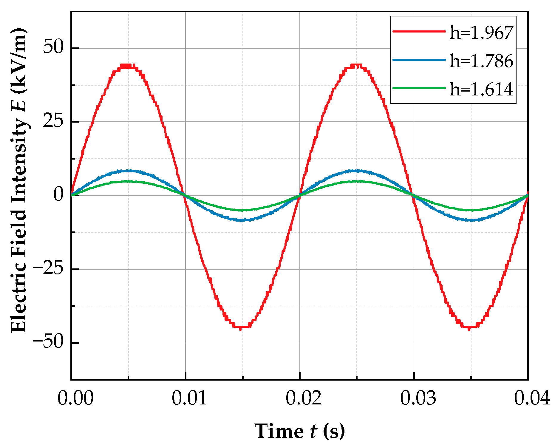
| Region (m) | Node Position (m) |
|---|---|
| x1 | 1.957 |
| x2 | 1.786 |
| x3 | 1.614 |
Disclaimer/Publisher’s Note: The statements, opinions and data contained in all publications are solely those of the individual author(s) and contributor(s) and not of MDPI and/or the editor(s). MDPI and/or the editor(s) disclaim responsibility for any injury to people or property resulting from any ideas, methods, instructions or products referred to in the content. |
© 2023 by the authors. Licensee MDPI, Basel, Switzerland. This article is an open access article distributed under the terms and conditions of the Creative Commons Attribution (CC BY) license (https://creativecommons.org/licenses/by/4.0/).
Share and Cite
Liao, W.; Yang, Q.; Ke, K.; Qiu, Z.; Lei, Y.; Jiao, F. Non-Intrusive Voltage-Inversion Measurement Method for Overhead Transmission Lines Based on Near-End Electric-Field Integration. Energies 2023, 16, 3415. https://doi.org/10.3390/en16083415
Liao W, Yang Q, Ke K, Qiu Z, Lei Y, Jiao F. Non-Intrusive Voltage-Inversion Measurement Method for Overhead Transmission Lines Based on Near-End Electric-Field Integration. Energies. 2023; 16(8):3415. https://doi.org/10.3390/en16083415
Chicago/Turabian StyleLiao, Wei, Qing Yang, Kun Ke, Zhenhui Qiu, Yuqing Lei, and Fei Jiao. 2023. "Non-Intrusive Voltage-Inversion Measurement Method for Overhead Transmission Lines Based on Near-End Electric-Field Integration" Energies 16, no. 8: 3415. https://doi.org/10.3390/en16083415