


Thermal-Hydraulic-Mechanical (THM) Modelling of Short-Term Gas Storage in a Depleted Gas Reservoir—A Case Study from South Germany †


Abstract
:1. Introduction
2. Methodology
2.1. Hydraulic Model
2.2. Thermal Model
2.3. Coupled Thermal-Hydraulic-Mechanical (THM) Modelling
2.3.1. Effective Stress and Poroelasticity
2.3.2. Simulation Concept and Governing Equations
2.4. ECLIPSETM_VISAGETM THM Modelling
3. Case Study
4. Modelling
4.1. Modelling Scenarios
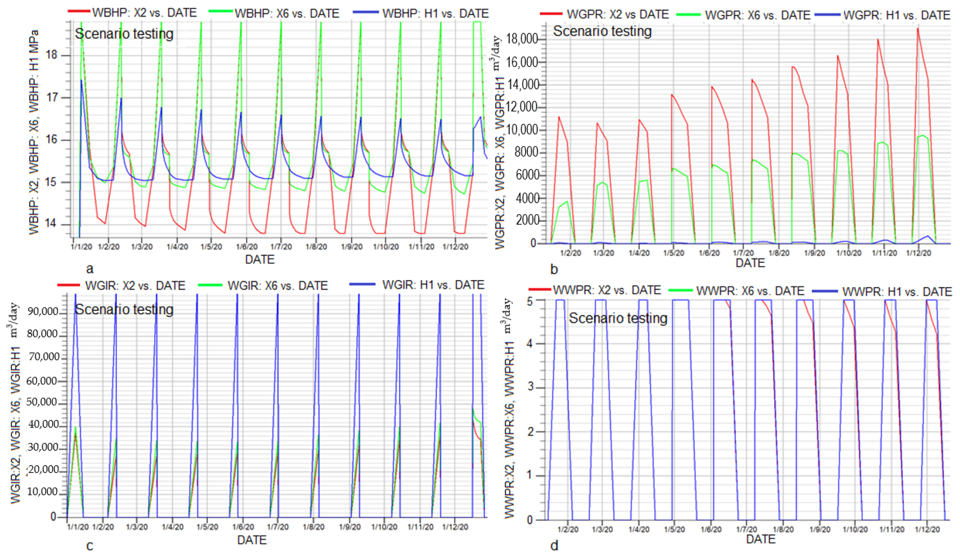
4.2. Case A
Results
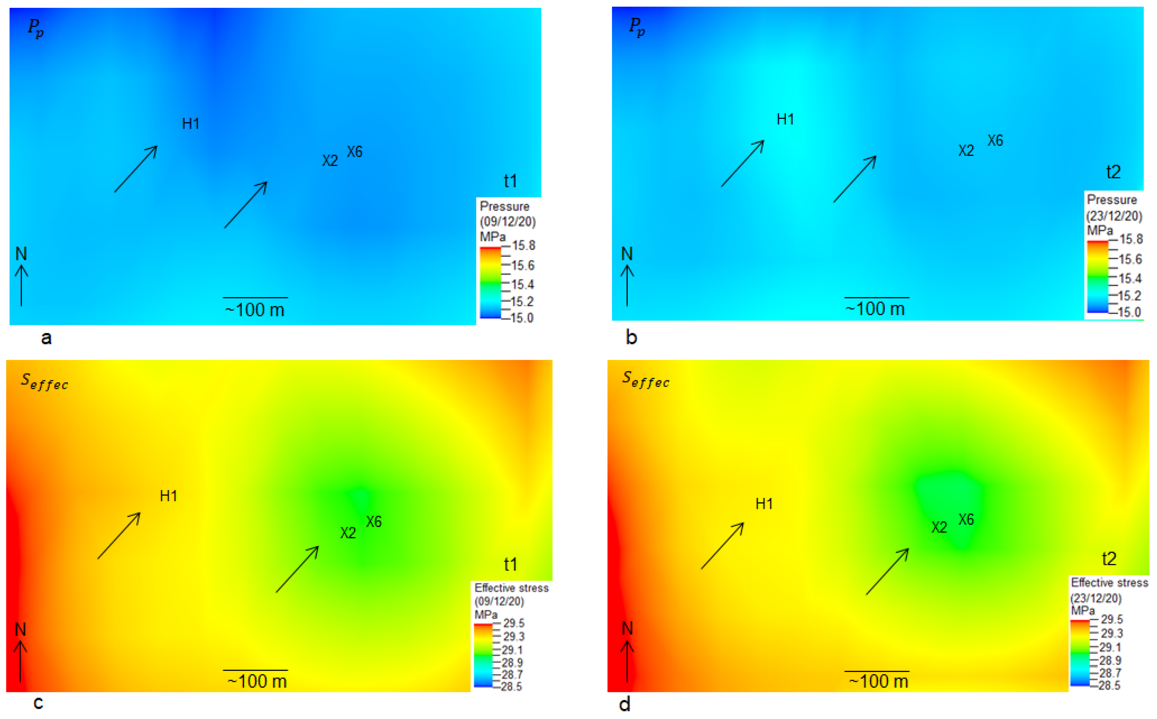
4.3. Case B
4.3.1. Results
4.3.2. Real World Cases
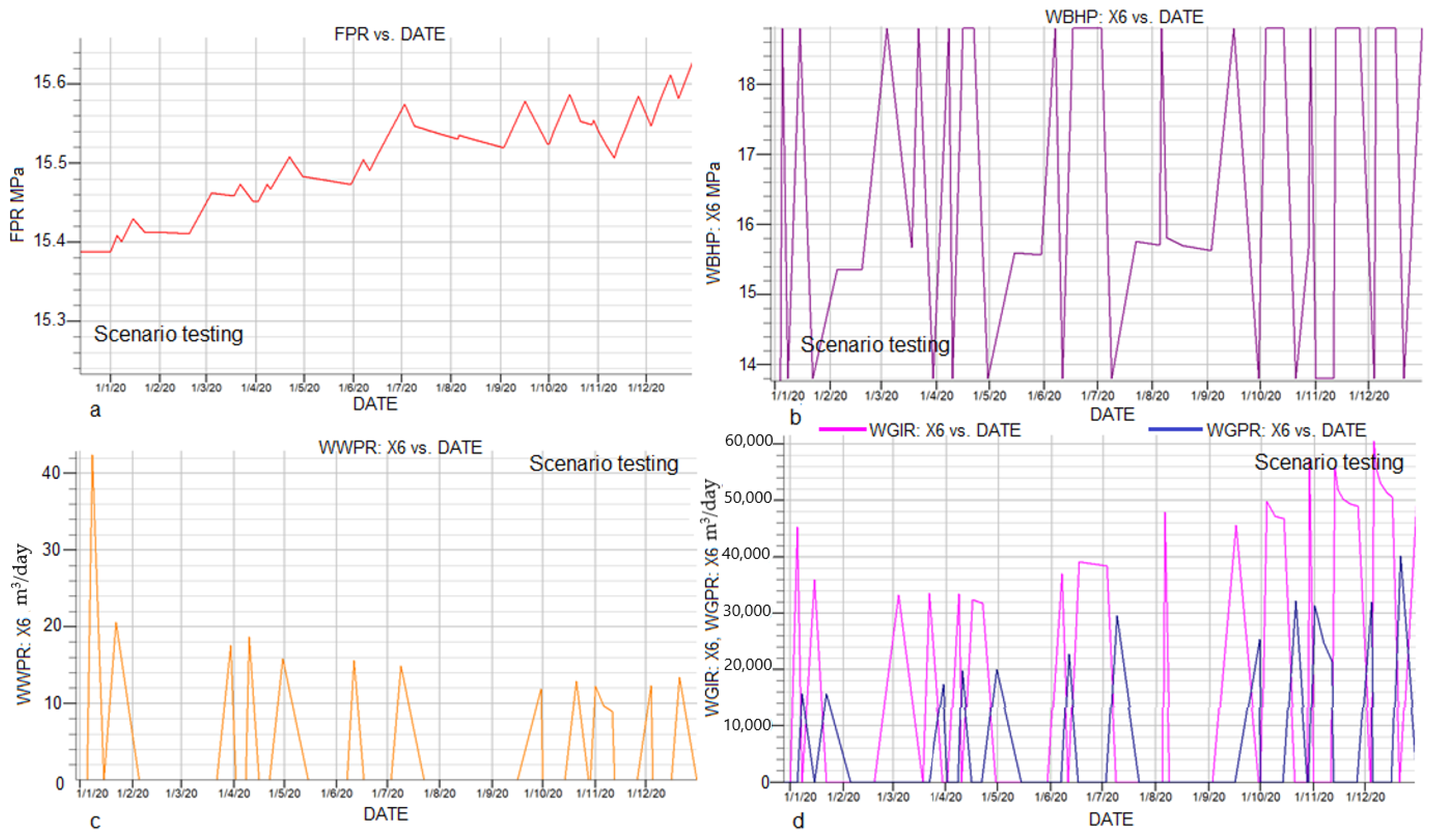
4.4. Case C
Results
4.5. Case D
Results
5. Thermal Analysis
6. Potential Fault Reactivation Analyses
6.1. Model Setup
6.2. Results
6.3. Safe Injection Rate for Safe Storage Capacity
6.4. Storage Capacity of Power-to-Gas and Gas-to-Power
7. Discussions
7.1. Hydraulic Model
7.2. THM Coupled Modelling
8. Conclusions
Perspectives
Author Contributions
Funding
Data Availability Statement
Acknowledgments
Conflicts of Interest
References
- Teatin, P.; Castelletto, N.; Ferronato, M.; Gambolati, G.; Janna, C.; Cairo, E.; Marzorati, D.; Colombo, D.; Ferretti, A.; Bagliani, A.; et al. Geomechanical response to seasonal gas storage in depleted reservoirs: A case study in the Po River basin, Italy. J. Geophys. Res. AGU J. 2011, 116, 21. [Google Scholar] [CrossRef]
- Tenthorey, E.; Vidal-Gilbert, S.; Backe, G.; Puspitasari, R.; Pallikathekathil, Z.; Maney, B.; Dewhurst, D. Modelling the geomechanics of gas reservoir: A case study from the Iona gas field, Australia. Int. J. Greenh. Gas Control 2013, 13, 138–148. [Google Scholar] [CrossRef]
- Aminian, K.; Brannon, A.; Ameri, S. Gas storage in a depleted gas/condensate reservoir in the appalachian basin. In Proceedings of the SPE Eastern Regional Meeting, Canton, OH, USA, 11–13 October 2006. [Google Scholar]
- Juez-Larre, J.; Remmelts, G.; Breunese, J.; Van Gessel, S.Q.; Leeuwenburgh, O. Using underground gas storage to replace the swing capacity of the giant natural gas field of Groningen in the Netherlands. A reservoir performance feasibility study. J. Pet. Sci. Eng. 2016, 145, 34–53. [Google Scholar] [CrossRef]
- Industry, D.O.T.A. Meeting the Energy Challenge: A White Paper on Energy; Her Majesty’s Stationary Off.: Norwich, UK, 2007. [Google Scholar]
- Zhang, J.; Fang, F.; Lin, W.; Gao, S. Research on Injection-Production Capability and Seepage Characteristics of Multi-Cycle Operation of Underground Gas Storage in Gas Field—Case Study of the Wen 23 Gas Storage. Energies 2020, 13, 17. [Google Scholar] [CrossRef]
- Kuncir, M.; Chang, J.; Mansdorfer, J.; Dougherty, E. Analysis and optimal design of gas storage reservoirs. In Proceedings of the SPE Eastern Regional Meeting, Pittsburgh, PA, USA, 6–10 September 2003; pp. 1066–1076. [Google Scholar]
- Mazarei, M.; Davarpanah, A.; Ebadati, A.; Mirshekari, B. The feasibility analysis of underground gas storage during an integration of improved condensate recovery processes. J. Pet. Explor. Prod. Technol. 2019, 9, 397–408. [Google Scholar] [CrossRef] [Green Version]
- Dharmananda, K.; Kingsbury, N.; Singh, H. Underground gas storage: Issues beneath the surface. In Proceedings of the SPE Asia Pacific Oil and Gas Conference and Exhibition, Perth, Australia, 18–20 October 2004; pp. 10–17. [Google Scholar]
- Abedin, M.Z.; Henk, A. Building 1D and 3D Mechanical Earth Models for Underground Gas Storage—A Case Study from the Molasse Basin, Southern Germany. Energies 2020, 13, 21. [Google Scholar]
- Khaksar, A.; White, A.; Rahman, K.; Burgdorff KOllarves, R.; Dunmore, S. Geomechanical Evaluation for Short Term Gas Storage in Depleted Reservoirs. In Proceedings of the 46th US Rock Mechanics/Geomechanics Symposium, Chicago, IL, USA, 24–27 June 2012. [Google Scholar]
- Bachmann, G.H.; Müller, M.; Weggen, K. Evolution of the Molasse Basin (Germany, Switzerland). Tectonophysics 1987, 137, 77–92. [Google Scholar] [CrossRef]
- Dake, L.P. Fundamentals of Reservoir Engineering; Elsevier Scientific Pub. Co.: Amsterdam, The Netherlands, 1978. [Google Scholar]
- Dai, W.J.; Gan, Y.X.; Hanaor, D. Effective Thermal Conductivity of Submicron Powders: A Numerical Study. Appl. Mech. Mater. 2015, 846, 500–505. [Google Scholar] [CrossRef]
- Settari, A.; Mourits, F. A Coupled Reservoir and Geomechanical Modeling System. SPE J. 1998, SPE 50939, 219–226. [Google Scholar] [CrossRef]
- Tortike, W.; Farouq, A.S. Reservoir Simulation Integrated with Geomechanics. J. Can. Pet. Technol. 1993, 5, 28–37. [Google Scholar] [CrossRef]
- Jalali, M.R.; Dusseault, M.B. Coupling Geomechanics and Transport in Naturally Fractured Reservoirs. Int. J. Min. Geol. Eng. (IJMGE) 2012, 46, 105–131. [Google Scholar]
- Mainguy, M.; Longuemare, P. Coupling Fluid Flow and Rock Mechanics: Formulation of the Partial Coupling between Reservoir and Geomechanical Simulators. Oil Gas Sci. Technol. 2002, 57, 355–367. [Google Scholar] [CrossRef] [Green Version]
- Perkins, T.K.; Gonzalez, J.A. The Effect of Thermoelastic Stresses on Injection Well Fracturing. Soc. Pet. Eng. 1985, 25, 78–88. [Google Scholar] [CrossRef]
- Geertsma, J. Problems of Rock Mechanics in Petroleum Production Engineering. First Congr. Int. Soc. Rock Mech. 1966, 1, 585–594. [Google Scholar]
- Skempton, A. The Pore Pressure Coefficients A and B. Geotechnique 1954, 4, 143–147. [Google Scholar] [CrossRef]
- Geertsma, J. The Effect of Pressure Decline on Volumetric Changes of Porous Rocks. Trans. AIME 1957, 201, 331–340. [Google Scholar] [CrossRef]
- Van der Knaap, W. Nonlinear Behavior of Elastic Porous Media. Trans. AIME 1959, 216, 179–187. [Google Scholar] [CrossRef]
- Nur, A.; Byerlee, J. An Exact Effective Stress Law for Elastic Deformation of Rock with Fluid. J. Geophys. Res. 1971, 76, 6414–6418. [Google Scholar] [CrossRef]
- Ghaboussi, J.; Wilson, E. Flow of Compressible Fluid in Porous Elastic Media. Int. J. Numer. Methods Eng. 1973, 5, 419–442. [Google Scholar] [CrossRef]
- Rice, J.; Cleary, M. Some Basic Stress-Diffusion Solutions for Fluid Saturated Elastic Porous Media with Compressible Constituents. Rev. Geophys. Space Phys. 1976, 14, 227–241. [Google Scholar] [CrossRef]
- Huan, X.; Xu, G.; Zhang, Y.; Sun, F.; Xue, S. Study on Thermo-Hydro-Mechanical Coupling and the Stability of a Geothermal Wellbore Structure. Energies 2021, 14, 649. [Google Scholar] [CrossRef]
- Rutqvist, J.; Wu, Y.; Tsang, C.F.; Bodvarsson, G. A modeling approach for analysis of coupled multiphase fluid flow, heat transfer, and deformation in fractured porous rock. Int. J. Rock Mech. 2002, 39, 429–442. [Google Scholar] [CrossRef]
- Pang, M.; Xu, G.; Sun, F.; Xue, S.; Wang, Y. Formation Damage and Wellbore Stability of Soft Mudstone Subjected to Thermal–Hydraulic–Mechanical Loading. J. Eng. Sci. Technol. 2019, 12, 95–102. [Google Scholar] [CrossRef]
- Hu, L.; Winterfeld, P.H.; Fakcharoenphol, P.; Wu, Y.S. A novel fully-coupled flow and geomechanics model in enhanced geothermal reservoirs. J. Pet. Sci. Eng. 2013, 107, 1–11. [Google Scholar] [CrossRef]
- Tran, D.; Nghiem, L.; Buchanan, L. Improved Iterative Coupling of Geomechanics with Reservoir Simulation; Society of Petroleum Engineers: Houston, TX, USA, 2005. [Google Scholar]
- Frey, C. Ministerin Hendricks: Wir Haben im Gegenteil Sogar Gigantische Stromüber-Schüsse. 2018. Available online: https://eike-klima-energie.eu/2018/01/07/ministerin-hendricks-wir-haben-im-gegenteil-sogar-gigantische-stromueberschuesse/?print=pdf (accessed on 1 June 2020).
- Burger, B. Fraunhofer ISE Fraunhofer ISE, Freiburg. 2018. Available online: https://www.ise.fraunhofer.de/content/dam/ise/de/documents/publications/studies/daten-zu-erneuerbaren-energien/Stromerzeugung_2017.pdf (accessed on 1 June 2020).
- Carter, G.F.; Paul, D.E. Materials Science & Engineering, Materials Park Ohio; ASM International: Novelty, OH, USA, 1991. [Google Scholar]
- Fjaer, E.; Holt, R.M.; Horsrud, P.; Raaen, A.M.; Risnes, R. Petroleum Related Rock Mechanics; Elsevier Science: Oxford, UK, 2008; p. 514. [Google Scholar]
- Terzaghi, K. Theoretical Soil Mechanics; Chapman and Hall Limited: London, UK, 1948. [Google Scholar]
- Zoback, M. Reservoir Geomechanics; Cambridge University Press: Cambridge, UK, 2007; p. 449. [Google Scholar]
- Chen, Z.R. Poroelastic model for induced stresses and deformations in hydrocarbon and geothermal reservoirs. J. Pet. Sci. Eng. 2012, 80, 41–52. [Google Scholar] [CrossRef]


| Modelling Scenarios | Subdivisions | Input Parameters | ||||
|---|---|---|---|---|---|---|
| WBHP upper limit (MPa) | WBHP lower limit (MPa) | WGIR (m3/day) | WGPR (m3/day) | |||
| Short-term (weekly) cases | Case A (with water-cut 5 m3/day) | With three wells (two vertical wells, one horizontal well) | 18.8 | 13.8 | 100,000 | 100,000 |
| Case B (without limited water-cut) | With three wells (two vertical wells and one horizontal well) | 18.8 | 13.8 | 100,000 | 100,000 | |
| Real-world cases | Case C (with water-cut 5 m3/day) | With one well | 18.8 | 13.8 | 100,000 | 100,000 |
| Case D (without limited water-cut) | With one well | 18.8 | 13.8 | 100,000 | 100,000 | |
| Modelling Scenarios | Subdivisions | Results | ||
|---|---|---|---|---|
| Pore pressure changes | Effective stress changes | |||
| Short-term (weekly) cases | Case A | With three wells (two vertical wells, one horizontal well) | +0.3 MPa +300 KPa | −0.3 MPa −300 KPa |
| Case B | With three wells (two vertical wells, one horizontal well) | +0.4 MPa +400 KPa | −0.4 MPa −400 KPa | |
| Real-world cases | Case C | With one well | +0.6 MPa +600 KPa | −0.6 MPa −600 KPa |
| Case D | With one well | +0.6 MPa +600 KPa | −0.6 MPa −600 KPa | |
| m3 Natural Gas | kWh Power |
|---|---|
| 1 | 8.816 |
| 0.113 | 1 |
Disclaimer/Publisher’s Note: The statements, opinions and data contained in all publications are solely those of the individual author(s) and contributor(s) and not of MDPI and/or the editor(s). MDPI and/or the editor(s) disclaim responsibility for any injury to people or property resulting from any ideas, methods, instructions or products referred to in the content. |
© 2023 by the authors. Licensee MDPI, Basel, Switzerland. This article is an open access article distributed under the terms and conditions of the Creative Commons Attribution (CC BY) license (https://creativecommons.org/licenses/by/4.0/).
Share and Cite
Zain-Ul-Abedin, M.; Henk, A. Thermal-Hydraulic-Mechanical (THM) Modelling of Short-Term Gas Storage in a Depleted Gas Reservoir—A Case Study from South Germany. Energies 2023, 16, 3389. https://doi.org/10.3390/en16083389
Zain-Ul-Abedin M, Henk A. Thermal-Hydraulic-Mechanical (THM) Modelling of Short-Term Gas Storage in a Depleted Gas Reservoir—A Case Study from South Germany. Energies. 2023; 16(8):3389. https://doi.org/10.3390/en16083389
Chicago/Turabian StyleZain-Ul-Abedin, Muhammad, and Andreas Henk. 2023. "Thermal-Hydraulic-Mechanical (THM) Modelling of Short-Term Gas Storage in a Depleted Gas Reservoir—A Case Study from South Germany" Energies 16, no. 8: 3389. https://doi.org/10.3390/en16083389