A Review of Wind Clustering Methods Based on the Wind Speed and Trend in Malaysia

Abstract

Wind mapping has played a significant role in the selection of wind harvesting areas and engineering objectives. This research aims to find the best clustering method to cluster the wind speed of Malaysia. The wind speed trend of Malaysia is affected by two major monsoons: the southwest and the northeast monsoon. The research found multiple, worldwide studies using various methods to accomplish the clustering of wind speed in multiple wind conditions. The methods used are the k-means method, Ward’s method, hierarchical clustering, trend-based time series data clustering, and Anderberg hierarchical clustering. The clustering methods commonly used by the researchers are the k-means method and Ward’s method. The k-means method has been a popular choice in the clustering of wind speed. Each research study has its objectives and variables to deal with. Consequently, the variables play a significant role in deciding which method is to be used in the studies. The k-means method shortened the clustering time. However, the calculation’s relative error was higher than that of Ward’s method. Therefore, in terms of accuracy, Ward’s method was chosen because of its acceptance of multiple variables, its accuracy, and its acceptable calculation time. The method used in the research plays an important role in the result obtained. There are various aspects that the researcher needs to focus on to decide the best method to be used in predicting the result.

1. Introduction

Wind clustering plays an important role in determining the various aspects of the research objective, such as energy, engineering, and public safety. Therefore, the usage of the relevant clustering method is basically determined by the objective of the study and the parameters involved in the study. The sensitivity of the data also plays an important role in determining the method of clustering. It is important for the researcher to have an expectation of what the result should be and will be so that the method can be used efficiently.

This paper focuses on a comparison of the clustering methods used by researchers in terms of wind speed clustering. The areas considered in this paper are in Malaysia, Qatar, France, Iran, Turkey, the United States, India, South Africa, Switzerland, and Columbia.

The winds in Malaysia are influenced by two monsoon seasons: the southwest monsoon from late May to September and the northeast monsoon of Peninsular Malaysia from November to March. The heavy rain to the east of Peninsular Malaysia and of western Sarawak is caused by the northeast monsoon, whereas the southwest brings drought to the nation [1].

Figure 1 shows the northeast monsoon storms; the east of Peninsular Malaysia and Mersing are the windiest areas of Peninsular Malaysia. Therefore, according to various wind energy potential research studies in Malaysia, Mersing is often the best location for wind farming [2].

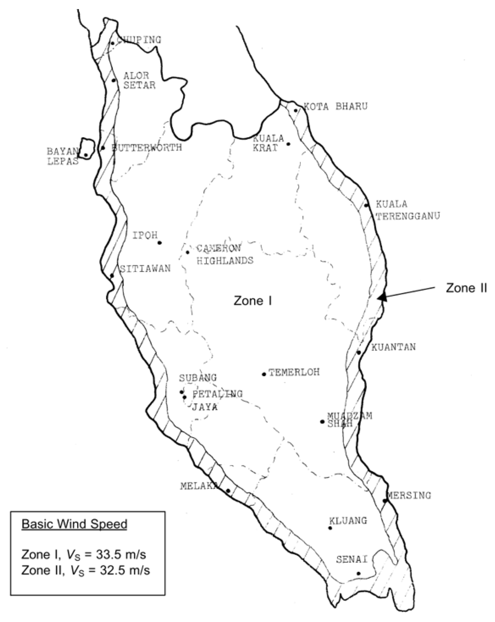
The monitoring of the wind speed trend is crucial for the prediction of future events or in seeing the continuity of the wind supply in certain areas. For example, the mapping conducted and adopted by the Malaysian Standard Code of Practice on Wind Loading for Building Structure uses mean wind speed. The standard is used by engineers in Malaysia, especially mechanical engineers and those involved with civil structures, to predict the wind speed in such areas as telecommunication antenna deployment. The mean wind speed usage may increase in a given year, as previously reported by Young in 2011. Figure 2 shows the recommendation by the Malaysian Standard on Basic Wind Speed with regard to a mean wind speed of 33.5 m/s [3].

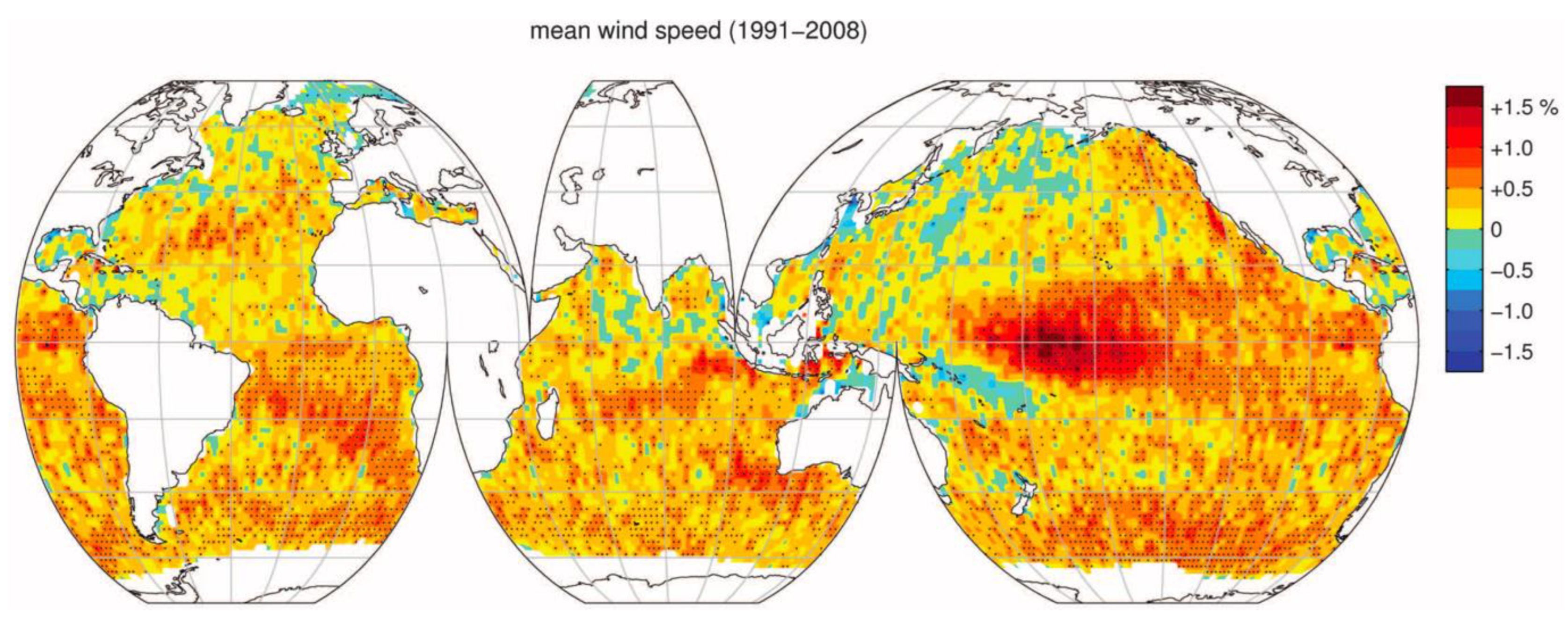
The global trends show that wind speed is increasing. Based on research in 2011, the global wind speed is increasing, indicating that extreme events are growing faster than the mean condition. The wind speed of most of the world’s oceans has increased by at least 0.25% to 0.5% per year. The strongest increasing trend was found in the southern hemisphere, and the northern hemisphere, especially the central North Pacific, shows a negative trend in wind speed. The wind speed increase in the central North Pacific was less than 0.25%, and some areas show a negative trend. As shown in Figure 3 below, the area surrounding Malaysia is also experiencing an increasing trend, especially in the southwest of Malaysia, where the southern Indian Ocean is located [4].

A study conducted in 2019 confirmed the above research by Young in 2011. As shown in Figure 4a, the research found that the global mean annual wind speed had increased for the previous ten years and that the pattern was increasing yearly. The Asian mean annual wind speed is also showing an increasing pattern. However, the wind speed in the Asian region began to increase earlier than the global speed. As shown in Figure 4b, the increase in wind speed in the Asian region started as early as 2002, whereas the global mean annual wind speed has been increasing since 2010. The research uses the diagnostic statistic for regression, which includes the goodness of fit, R², and the Pearson correlation coefficient, P. A Pearson correlation coefficient of less than 0.001 was considered be satisfactory in this study. However, the research found oscillation patterns that decreased the global wind speed; therefore, according to this research, wind energy production may decrease in the future [5].

In 2003, a study was conducted on the coastline of Peninsular Malaysia. The study focuses on analyzing the annual vector mean wind speed and direction according to two seasons, i.e., the northeast and southwest monsoons. The wind direction was northeast during the northeast monsoon season and southwest during the southwest monsoon season [6].

Research conducted in 2015 by Kok et al. found that the dynamics of the wind stress system had an important influence on the physical characteristics of the sea. The study used a wind stress curl to examine the mechanism responsible for the formation of the thermal front during both Malaysian monsoon seasons [7].

The positive and negative values of the wind stress curl cause cyclonic and anti-cyclonic motion in the northern hemisphere. This action causes divergence of the convergence in the surface layer of seawater. Therefore, the cooler or warmer water from the deep rises and replaces the diverging or converging water. This results in the upwelling and downwelling of the seawater. This upwelling is caused by the wind, which makes the water close to shore cooler [8].

Therefore, with regard to all of the wind characteristics mentioned, there is a need for wind trend monitoring and clustering, especially in Malaysia. Factors such as global warming have increased the temperature of the sea, causing the fluctuation in the global wind speed [9]. When wind standards commenced in 2002 in Malaysia, the need for wind clustering was foreseen; wind clustering can increase the accuracy of wind mapping and wind forecasting in Malaysia.

It is important for engineers and wind experts to able to see the wind trend and clustering according to objectives such as those considering area or demand. Each objective can show different results, which also depend on the method of clustering used. This paper aims to investigate the best method to cluster the wind trend. The specific objective is to determine the best method to cluster the wind trend in relation to the Peninsular Malaysia and Borneo regions.

2. Methodology of Wind Speed Clustering

2.1. Wind Speed Trend Observation

Wind speed observation has been conducted by the researchers based on various objectives. The research which uses the method of observation of wind speed trends is that of the wind energy researchers. Wind energy research requires wind trend observations to ensure the continuity of the wind supply that powers the wind harvesting equipment.

Research to evaluate the wind energy potential in Peninsular Malaysia was conducted from 2007 to 2009 by Masseran et al. at 10 wind stations. The research, which focuses on the wind speed persistence in Peninsular Malaysia, is based on hourly data. The research found that for Peninsular Malaysia, the hourly wind speed for the wind station exhibits stationarity state. The smallest hourly wind speed observed at the Chuping station and Mersing station showed its suitability for the generation of energy due to its hourly wind trend. Therefore, the research shows the importance of wind trend observation in wind energy research methodology. Figure 5 below shows the wind speed trend for one week at Ipoh wind station, Perak [10].

The wind trend also uses research conducted in Qatar by Aboobacker in 2021. The research uses monthly mean data to simulate the trend of the wind speed and to further estimate the wind power produced in the area [11]. The research focuses on the wind around the Arabian gulf coast and focuses on the Qatar peninsula. The research found that the highest wind speed was located in offshore Ruwais. Offshore Ruwais was found to be the windiest location and to have the highest mean wind speed.

Table 1. Wind speed statistics at onshore and offshore locations from 1979 to 2018 [11].

Region	Locations	Geographical Co-Ordinates		Wind Speed (m/s)			% of Exploitable Wind Speed
		Longitude (° E)	Latitude (° N)	Maximum	Mean	Standard Deviation
Onshore	Mesaieed	51.5828	25.0444	15.4	4.6	2.3	73.9
	Al Khor	51.4394	25.7534	16.2	5.1	2.6	77.1
	Al Ruwais	51.2202	26.0690	15.9	4.9	2.5	74.7
	Dukhan	50.8398	25.3355	15.7	4.9	2.4	77.5
Offshore	Doha	51.7970	25.2755	15.5	5.1	2.5	78.5
	Ras Laffan	51.6146	26.0131	16.5	5.2	2.7	76.5
	Al Ruwais	51.2992	26.2822	16.9	5.5	2.8	78.4
	Dukhan	50.7251	25.4767	16.1	5.0	2.4	78.2

below shows the wind speed statistics at the research locations from 1979 to 2018 [11].

The trend observations were also conducted by research which showed that there were similarities in the onshore and offshore wind trends, as shown in Figure 6. However, the two windiest stations were Ras Laffan and Ruwais. The research using mean wind speed trend observations was similar to the current research in terms of the finding of the strongest wind recorded in the area. Therefore, the method of observation by trend was applicable in finding the windiest area or the area with the strongest wind.

In 2012, Tiang and Ishak studied the wind speed at the measurement site of Bayan Lepas, Pulau Pinang, from January to December 2008. The study used wind trend observation to assess the potential wind energy in Pulau Pinang. By observing the trend of the wind speed, the researchers were able to find the windiest period in Pulau Pinang. Based on the findings, the maximum wind speed in Pulau Pinang was achieved in September, and the slowest was recorded in November. Using the trend observation, the researchers were able to determine the months in Pulau Pinang that were the windiest and had the highest wind speed; these were May, July, and September. The causes of the higher wind speed period were the southwest monsoon season and the geographical location of Pulau Pinang. Figure 7 below shows the monthly mean wind speed trend in 2008 from July to October [12].

However, in terms of the engineering purposes, the wind trend observation focused more on the sudden spike in wind speed and the highest wind speed recorded in the research area. The research conducted by Shanmugasundaram et al. in 1998 was based on the tropical cyclone wind condition which occurred in June and December 1996. The research came out with a wind trend observation of the cyclone which indicated the highest mean and maximum wind speed recorded during the event. The wind speed trend observation helped the researchers to locate the maximum wind speed during the event and to calculate the damping ration increase for the 52 m steel lattice tower. Figure 8 below shows the mean and maximum wind speeds during the cyclone of the year 1996 [13].

The research which was based on the air pollution also used the wind trend analysis to simulate the severity of the pollution affecting the area. The direction and speed of the wind plays an important role in the air pollution effect. In 2016, Sokolov et al. conducted a cluster analysis of the atmospheric dynamics and pollution transport in the coastal area of industrialized Dunkerque in northern France. The research aimed to determine the trajectories in the context of pollution transport. The trajectories were based on the largest and most dispersed areas of low wind speeds, which make the pollution worse. The data of this research were based on the meteorological data of the wind speed and its direction and pollution measurements. The wind trend observation was visualized based on the wind rose. The wind rose modeling was successful in showing the trend in terms of the direction and the wind speed at Maregraph station. Figure 9 below shows the wind rose modeling for Maregraph station from 1st May to 1st October 2006 [14].

Therefore, the wind trend observation requirement is based on the objective of the research. The wind trend observation can assist with multiple factors and can contribute to the objective of the research. However, wind trend observation for a longer period may require grouping or clustering to ease the analysis and to localize the wind trend according to the area.

2.2. Clustering Wind Speed

2.2.1. Linkage–Ward Clustering Method

The probabilistic wind speed clustering was used in the study cases at Khaaf, Iran, in 2018 [15]. Azizi et al., reported using the Linkage–Ward clustering method to cluster the wind speed in the area. The research reported that the usage of the Ward clustering method was higher in accuracy compared to the k-means method. The Ward method, however, was more complex than the k-means method. For two years, the study used the measured wind speed time of 60 min in the wind stations around Binalood, Iran. The wind stations vary in height, soil, and distance to residential areas. The focus of the study was to select the proper site to install the wind turbine in Binalood. Therefore, the study focuses on the windiest area, which can be correlated with the current study. Although the study also used the Linkage–Ward clustering method instead of k-means, the Linkage–Ward clustering method required even more computational effort to solve.

The research found that the Linkage–Ward clustering method was the most common and accurate for use in the study. The method calculated the dissimilarity between clusters based on the centroid of the cluster, as shown in (1)

$$d_{i+j,k}=a{d}_{ik}+a{d}_{jk}+b{d}_{ij}+c\left|d_{ik}-d_{jk}\right|,$$

(1)

where d_ik, d_jk, d_ij are the pairwise distances between the clusters i and k, j and k, and i and j. i, j, k are the indexes of the clusters. n_i, n_j, n_k are the numbers of members within clusters i, j, and k, respectively.

$$a=\frac{n_i+n_k}{n_i+n_j+n_k},b=\frac{n_j+n_k}{n_i+n_j+n_k}$$

(2)

where a and b are defined as (2), and c = 0 in the Linkage–Ward clustering method. a and b are the parameters, which depend on the cluster size to determine the clustering algorithm, with a distance between clusters of d_ij.

The clusters which have the lowest increase in distance between the cluster centroids (1) are combined. The Ward method uses the objective function in the sum of the squares from the points to the centroids of the clusters. Figure 10 below shows the step-by-step algorithm of Linkage–Ward clustering.

The calculation above will result in the lowest increase in the cost function of (1) and in the combination. The method uses the objective function in the sum of the squares from the points to the centroids of the clusters. Figure 11 below shows the average wind speed value sample at a 40 m height with 10 min intervals in the study area. The color lines indicate 50 days chosen randomly by the researchers [15].

The researchers found the centroid of the cluster where the study was able to find the mean of the wind speed earlier in the research. This is a reverse method to find the centroid of the cluster and may affect the result. Figure 12 below shows the cluster centers of the measured wind speed.

The number of clusters was chosen by calculating the error of the cluster’s centroid and its member. As expected, a small number of clusters brings out the dissimilar object group. The optimal number of clusters is important to ensure the effectiveness and the accuracy of the data. The Euclidian error between each cluster is calculated as in (3).

$$error={\sum }_{i=1}^{N_{Cluster}}{\sum }_{j=1}^{n_j}|x_j-c_i|$$

(3)

where N_Cluster is the number of clusters, n_j is the number of members within cluster j, respectively, x is each observation in the dataset, and c_i is the centroid of cluster i.

The error calculation found that the minimum error obtained for this research was four clusters, as the calculation showed that only an 8% relative error was found. Therefore, the research used four clusters as the basis of the clustering for the dataset. Figure 13 below shows the error calculation result in determining the number of clusters.

Azizi et al. found that from the four clusters created, cluster 2 had the higher probability compared to the other clusters, at 38%. The higher probability occurrence suggests that cluster 2 is more suitable for wind farming. Figure 14 below shows the probability of occurrence of each cluster.

2.2.2. k-Means Approach for Wind Clustering

The annual wind speed patterns can be grouped when the study area is the same. Yesilbudak et al. conducted a clustering analysis of multidimensional wind speeds for 75 provinces in Turkey. The method used in the clustering was the k-means approach. In this research, the silhouette coefficient was used to determine the effectiveness of the distance measure. The analysis found that the prominent cities in terms of average wind speed were Canakkale and Mardin, located in cluster 4, where the mean cluster of silhouettes was 0.5224. On the other hand, cluster 1 contained Duzee, Amasya, and Siirt, which were determined to be poorly matched areas with the silhouette coefficients of 0.7294, 0.7198, and 0.7111. Figure 15 below shows the silhouette coefficients for k = 5 and the square Euclidean distance measure result [16].

In this research, the study mentioned k-means as one of the portioning methods in the literature. The k-means algorithm assumes that D is the dataset that contains n observations and k is the number of clusters. The k-means calculated the dissimilarity between each pair observation differently according to the distance measures. Four types of distance measures were used: squared Euclidean, city-block, cosine, and Pearson. Figure 16 below shows the k-means algorithm used in the study.

To determine the best distance measure, the silhouette coefficient varying between −1 and +1 was used for measuring the observation assigned to the clusters. The accuracy was defined by the silhouette coefficient closer to 1, which indicated that the observation belonged to its cluster. The silhouette was defined as in (4) below.

$$s\left(y_i\right)=\frac{b\left(y_i\right)-a\left(y_i\right)}{max\left\{a\left(y_i\right),b\left(y_i\right)\right\}}$$

(4)

where a(y_i) is the average dissimilarity of y_i and the element of (∈) S_k to all other y_j ∈ S_k, and b(y_i) is the minimum average of dissimilarity of y_i ∈ S_k to all other y_j ∈ S_l.

As shown in Figure 17, the study plots the annual wind speed data using star glyph plots. The plots shown in Figure 17 show the wind pattern of the 75 areas around Turkey. The analysis by the k-means algorithm with the silhouette coefficient gives a stronger clustering solution. The research found that using the square Euclidean distance measure gives a more accurate clustering result compared to the other three distance measuring methods. Therefore, the clustering result was obtained using the square Euclidean distance measure, as shown in

Table 2. The province categorized into each cluster by the k-means approach [16].

Cluster Name	Cluster Observations
Cluster 1	1, 4, 5, 9, 11, 12, 13, 17, 19, 23, 26, 28, 35, 36, 41, 44, 47, 50, 51, 54, 56, 60, 69, 72, 75
Cluster 2	7, 10, 15, 20, 21, 22, 30, 31, 32, 34, 49, 53, 58, 62, 64, 66, 67, 68, 70, 73, 74
Cluster 3	2, 3, 8, 14, 18, 27, 37, 39, 40, 42, 43, 46, 48, 52, 61, 63, 71
Cluster 4	16, 45
Cluster 5	6, 24, 25, 29, 33, 38, 55, 57, 59, 65

below.

Time series clustering has been widely used in predicting wind speed. For example, Kusiak et al. conducted wind speed clustering to predict the power output generation based on the wind speed. The researchers’ study was based on the long- and short-term prediction of power using the k-nearest neighbor (k-NN) algorithm [17].

In this research, multiple parameters were considered during clustering calculation. The parameters also made the clustering much more detailed and precise. Therefore, a clustering method that can cater for bigger variables has to be used for the clustering exercise to be successful.

Table 3. List of parameters selected for wind speed estimation [17].

Parameter Type	Parameter Name	Abbreviation	Symbol	Unit
Non-controllable	Wind speed	WS	v	m/s
Controllable	Blade pitch angle	BPA	x1
	Generator torque	GT	x2	Nm
Performance	Power output	PO	y1	kW
	Rotor speed	RS	y2	rpm

below shows the list of parameters used in the research by Kusiak et al.

However, the current wind speed data were unavailable during the study. Therefore, the prediction of the power generated from the wind speed was not validated [17].

In 2012, Andrew Clifton demonstrated the usage of k-means clustering to identify the relationship between the wind at turbine height and climate oscillation. The study used fourteen years of data from an 80 m tower at the National Wind Technology Center (NWTC) in Colorado. During the study, the k-means method of clustering identified four dominant wind flows in the area. The study first identifies the frequency of the wind direction. However, for the frequency study, the data are limited to the wind speed of 3.5 m/s and grouped into 5° and 1 m/s bins. The contours show the relative frequency in each bin on a linear scale. Figure 18 below shows the wind frequency visualized in contours.

The researcher applied the k-means clustering approach to zonal and meridional wind speeds. The k-means clustering splits N data points into k clusters and assumes that the data belong to the nearest mean value. The researcher repeated the clustering 100 times using a random initial centroid and generated an optimum set of centroids. The research used the function form of the “Statistics Toolbox” in the software MATLAB R2010b to generate the k-means analysis. Thereby, four dominant flows were found: the weak northerly (N), weak southerly (S), weak westerly (W(L)), and strong westerly flows. The clustering of the flows is shown in Figure 19 below [18].

The optimum number of clusters was obtained by Andrew Clifton’s research using the Bayesian information criterion (BIC) method. The BIC method increased the number of k to a point where k would not give a meaningful quality to the result. The method performs well in two-dimensional datasets, especially when using a machine learning application such as MATLAB [19]. Figure 20 below shows the variation of the normalized BIC value with the number of clusters, and the result shows that optimum number of k is 4.

2.2.3. Non-Parametric Approach Hierarchical Clustering

Guldal et al. used hierarchical clustering algorithms to cluster the wind speed and blow number, a parameter which causes evaporation in Lake Egirdir, Turkey. The research used a non-parametric approach of the hierarchical clustering algorithm where the monthly evaporation losses and the mean wind speeds with the blow number were clustered. The clustering method was determined by the mutual neighbor distance (MND) algorithm. Figure 21a shows the pattern labelled A, B, C, D, E, F, and G, which falls into three clusters. The clustering can be further refined using a single-link algorithm, as shown in Figure 21b [20].

Figure 21 shows the hierarchical clustering algorithm in a two-dimensional dataset. Figure 21a shows that there are seven observations, labelled as A, B, C, D, E, F, and G, in three clusters. Therefore, in Figure 21b, the dendrogram shows the grouping of seven patterns and the similarity levels of the observations. Figure 21b shows that the clustering can be broken into multiple levels. For example, level 1 comprises three clusters, (A, B and C), (D and E), and (F and G) [20].

The mutual neighbor distance (MND) used by this study is described in Figure 22 and by MND Equation (5) below;

$$MND(x_i,x_j)=NN(x_i,x_j)+NN(x_j,x_i)$$

(5)

where NN (x_i, x_j) is the neighbor number of x_j with respect to x_i. Figure 22 shows the example of MND. The neighbor nearest to A is B, and B is the nearest neighbor of A. Therefore, NN(A,B) = NN (B,A) = 1. The MND between A and B become 2 according to Equation (5) above. The NN (B,C) = 1, and the NN (C,B) = 2. Therefore, the MND (B,C) = 3.

The result from the above method shows both the similarity (S) levels (l) of S6 (l6) and S8 (l8) and the strong relation of the evaporation rate, R² (R² = 0.29 for wind speed change and evaporation rate), (R² = 0.85 for wind blow number and evaporation rate), for June, July, August, and September. The strongest relationship is the clustering at l = 6 (S6), as shown in Figure 23a; the detail of the similarity level S6 (l6) clusters analysis is shown in Figure 23b, where the coefficient of the evaporation rate is 0.96. Therefore, the clustering should determine different operation levels to make efficient operating decisions and accurate predictions. Furthermore, this prediction should produce scientific meaning by representing the actual object in the best way [20].

However, the research of Guldal et al. does not discuss the relative error or comparison between methods since the research only uses the non-parametric approach.

2.2.4. Trend-Based Time Series Data Clustering Using Statistical Model

The wind prediction method has been studied and revised with multiple hybrid methods to simplify and increase the accuracy of the algorithm. Kushwah et al. studied wind forecasting by using a time series. Wind components such as seasonal trends can be monitored in the time series application. In this research, the clustering method was based on the seasonal trend. As shown in Figure 24 below, the proposed model for wind speed prediction uses the trend as the major component during the study [21].

The study used standard deviation for data analysis. The result from the standard deviation analysis was then converted into a time series for clustering purposes. The wind prediction was evaluated in four models: the autoregressive integrated moving average (ARIMA), the generalized autoregressive score (GAS), a hybrid model of C-ARIMA, and a hybrid model of C-GAS. The finding was that both hybrid models performed better compared to the original model of ARIMA and GAS in terms of forecasting wind trends. Figure 25, in the left, middle, and right panels, shows the wind speed prediction using the GAS model for the first, second, and third clusters.

The result also shows that the mean absolute error (MAE) and root mean square error (RMSE) for the hybrid models are lower than the original, as shown in

Table 4. MAE and RMSE values using the ARIMA and clustered ARIMA models [21].

Dataset	ARIMA		CI-ARIMA		C2-ARIMA		C3-ARIMA
	MAE	RMSE	MAE	RMSE	MAE	RMSE	MAE	RMSE
#1	7.346	8.649	5.159	5.973	5.940	6.937	5.570	6.326
#2	4.675	5.972	7.029	8.43	4.191	5.206	4.726	6.047
#3	2.968	4.281	2.747	3.897	3.821	5.021	6.156	6.964
#4	6.593	6.976	6.374	6.757	9.113	9.383	13.893	14.061
#5	4.074	4.359	10.319	11.136	6.344	6.685	7.404	7.697
#6	5.558	7.124	5.563	7.254	5.653	7.331	5.679	7.241
#7	2.796	3.291	3.257	3.833	1.714	2.106	92.738	123.995
#8	4.246	4.95	3.362	4.049	3.554	4.252	4.88	5.645
#9	4.207	4.785	11.621	12.062	9.483	10.01	9.358	9.877
#10	3.455	3.771	2.528	2.869	4.725	4.983	2.294	2.591
#11	2.188	2.743	2.144	2.699	2.048	2.609	6.471	6.956
#12	4.751	6.593	4.22	4.808	11.128	12.232	3.917	4.949

MAE: mean absolute error; RMSE: root mean square error; ARIMA: autoregressive integrated moving average.

and

Table 5. MAE and RMSE values using the GAS and clustered GAS models [21].

Dataset	GAS		CI-GAS		C2-GAS		C3-GAS
	MAE	RMSE	MAE	RMSE	MAE	RMSE	MAE	RMSE
#1	5.017	5.767	2.955	3.398	6.324	7.377	6.454	7.342
#2	4.788	6.176	5.776	7.304	4.51	5.672	4.802	6.133
#3	3.003	3.82	13.468	15.224	1.785	2.395	2.887	3.356
#4	2.738	3.431	1.794	2.449	4.767	5.94	9.919	10.25
#5	5.212	5.373	6.928	7.107	8.11	8.579	7.266	7.559
#6	7.268	9.359	7.175	9.369	5.94	7.771	6.143	7.955
#7	1.851	2.599	3.155	3.47	1.715	2.016	5.188	5.402
#8	6.324	7.166	5.487	6.258	5.341	6.077	5.029	5.777
#9	7.068	8.019	5.52	6.553	4.321	5.37	7.387	8.227
#10	4.952	5.371	2.112	2.426	8.576	8.8	2.82	3.159
#11	2.474	3.164	2.988	3.468	2.42	3.078	8.334	8.76
#12	4.378	5.951	5.9	6.899	5.213	6.823	6.093	7.259

MAE: mean absolute error; RMSE: root mean square error; GAS: generalized autoregressive score. Bold numeric value of MAE and RMSE indicates that the prediction model corresponding to the column has the least prediction error and performed better on the Dataset representing that row.

below. The bolded numbers in the tables are the lowest error values obtained during the analysis [21].

The study above, however, did not reveal the result of the wind clustering and only reviewed the precision of both hybrid methods of wind forecasting.

In 2019, based on the Komsberg, South African area, research on the mean daily wind speed was conducted by Vuuren and Vermeulen. The study focuses on clustering the mean daily wind speed and comparing it with the customers’ demands. The research then further analyzed the tariff to optimize the siting areas for wind energy facilities. The study used multiple clustering algorithms to cluster wind resource datasets. The algorithms used were k-means, partitioning around medoids, the clustering large application algorithm, agglomerative clustering, the divisive analysis algorithm, and fuzzy c-means clustering. The research also used the Euclidean distance and Pearson correlation of the distance measurement. The research used the standard deviation method to obtain the mean high wind speed. Figure 26 shows the daily mean, median, and variance characteristics of the wind speed profiles for the REDZs for the 2013 period, using the standard deviation method [22].

The research used three types of clustering methods. The clustering methods were the k-means algorithm, the partitioning around medoids algorithm (PAM), and the clustering large application algorithm (CLARA). The k-means clustering algorithm result showed a non-overlapping cluster for the Komsberg wind speed profile. Figure 27 below shows a 2D representation of the variables through principal component analysis.

The research used a dendrogram to show the cluster assignment obtained by using the hierarchical agglomerative algorithm. Figure 28 below shows the clustering tree-like structure used to represent the four clusters assigned to the data based on the clustering method. Therefore, the mean wind speed can be visualized by the tree diagram and is easy to understand.

Based on the clustering analysis,

Table 6. Validation result for the various clustering algorithms.

Validation Method	Partitioning Clustering Algorithms			Hierarchical Clustering Algorithms		Advance Algorithms
	K-Means	PAM	CLARA	Agglomerative Clustering	DIANA	Fuzzy C-Means
Silhouette coefficient	0.44	0.48	0.52	0.45	0.47	0.45
Number of incorrect cluster assignments	14	6	2	26	4	16
Calinski-Harabasz Index	861.731	851.731	826.047	794.786	854.381	829.219
Average distance within clusters	4.436	4.423	4.516	4.584	4.446	4.433
Dunn index	0.0569	0.0340	0.0411	0.0455	0.0420	0.0410

below shows the validation result of the research. The result shows that the PAM and CLARA algorithm gave the best validation result. It was found that the CLARA algorithm reduced the algorithmic computing time of the large datasets without deceasing their accuracy. The CLARA algorithm also gave the highest silhouette coefficient. Therefore, it was concluded that CLARA algorithm was the most suitable method to use in this research.

2.2.5. Anderberg Hierarchical Clustering Method

In 1996, Kaufmann et al. used the hierarchical clustering method in research in which the wind speed was an absolute value with vector differences at the station. The research took place for a duration of one year in the city of Basel. The period reflected the diurnal and seasonal airflow variation in the complex terrain. The study analyzes the normalized hourly mean of the wind fields. The distances measured for the study were defined as the mean absolute values of the vector differences at all the stations involved [23]. The study is comparable to the study of Gassmann et al., in which they used Ward’s clustering method with distances of Euclidean measurement [24].

However, the method was found to be unsuitable for use in the study. Therefore, the study used the complete linkage method (Anderberg), which tended to build a group of similar size but focused on the ranking of the distances.

Table 7. Summary of the 15 clusters obtained by the complete linkage clustering method [23].

Cluster Number	Count	Relative Frequency	Mean Wind Speed (ms−1)	Std. Dev. (ms−1)
1	127	1.4%	1.7	0.60
2	166	1.9%	1.5	0.41
3	419	4.8%	2.1	0.71
4	30	0.3%	2.0	0.74
5	1692	19.3%	3.8	1.76
6	751	8.5%	2.8	1.19
7	637	7.3%	2.3	0.82
8	1643	18.7%	2.5	0.83
9	376	4.3%	1.9	0.61
10	580	6.6%	3.2	2.10
11	176	2.0%	1.3	0.27
12	407	4.6%	2.3	1.41
13	159	1.8%	1.4	0.39
14	1050	12.0%	1.9	0.59
15	571	6.5%	2.0	0.67
Total	8784	100.0%	2.6	1.39

below summarizes the result obtained in the study of Kaufmann et al., where 15 clusters were found based on the criteria given [23].

The study found that 15 clusters could be produced based on the analysis using complete linkage clustering. A clear diurnal variation of wind patterns was observed, and it fit with the physical mechanism of the mountain valley wind and the characteristics of the sample of the cluster for normalized wind vectors obtained during the study, as in Figure 29 below. The research, however, did not discuss the error analysis of the method used [23].

2.2.6. Other Methods of Data Clustering

Angosto et al. conducted a wind clustering analysis to predict atmospheric pollution. The research found five different wind patterns by using a two-step clustering analysis in the city of Cartagena. The analysis clustered the wind direction into five clusters. For example, the first cluster found that 6.5% of the cases of wind direction were north-northwest and north. The second cluster had wind of a south-southwest and south direction, which comprised 24.7% of the data. The method used in this research was a two-step clustering analysis procedure that used the hierarchical (average linkage) and non-hierarchical (k-means) methods [25].

There are other clustering algorithms, such as the density-based spatial clustering of application with noise (DBSCAN) and the autoregressive integrated moving average (ARIMA). Dokuz et al. used both the DBSCAN and the ARIMA algorithms in their research on wind speed forecasting. The study found that using both methods provided a better performance than using a single method. In addition, the hybrid method proved that the root mean square error (RMSE) decreased up to 20% [26].

3. Recommendation and Conclusions

As mentioned in the above topics, there are many methods of clustering used to cluster wind speed. The non-parametric hierarchical clustering using the mutual neighbor distance algorithm shows a complex method of clustering and an acceptable result. The method showed an efficient operating decision and made accurate predictions during research [20].

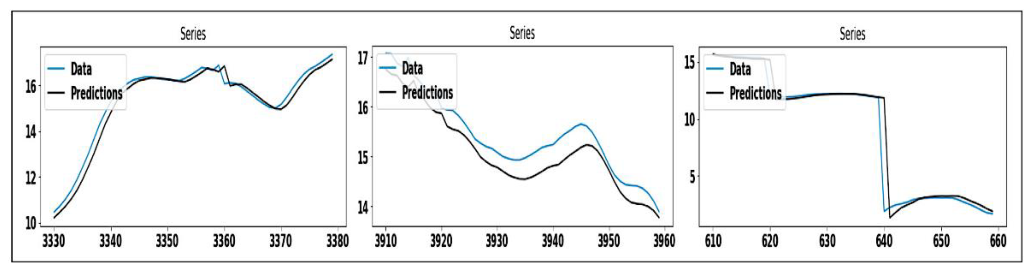
The trend-based time series clustering shows that the method produces excellent accuracy. Even though the research focuses on forecasting the wind speed, the study shows that the wind speed can be clustered according to its trend. This was shown in the research of Kushwah et al. for the yearly trend. Therefore, the trend can be predicted as it follows a seasonal pattern, and the application of this research is good for research with a localized wind speed trend prediction. The clustering using the trend-based method was successfully shown in the research of Vuuren et al., where the researchers successfully clustered the mean daily wind speeds for the high demand season using the clustering large application algorithm (CLARA).

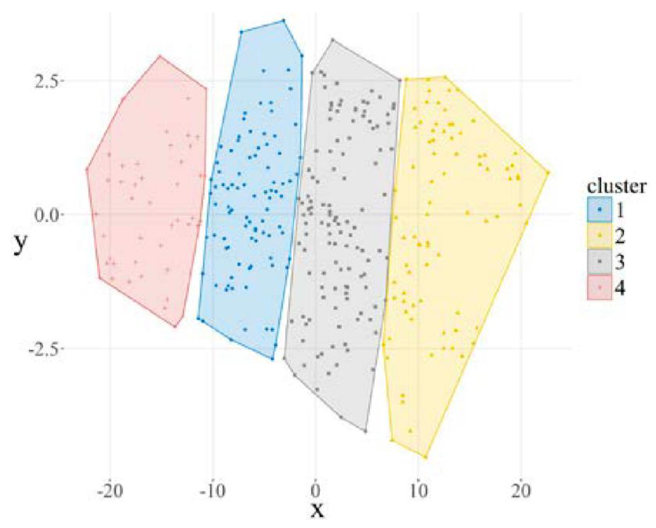
However, there are two main methods that the wind clustering researcher usually uses: the k-means and the Ward methods. Both methods are based on the k-value to determine the partition size of the cluster. The cluster size is important to the researcher when determining the number of desired clusters according to the research objective.

For the k-means method, the algorithm gives no guidance for the numbers of k. However, Ward’s method gives some partition sizes of k, which should be within the partition size of k + 1. Therefore, Ward’s method does not produce a sum of squares as small as that of the k-means method. Between the k-means method and Ward’s method, Ward’s method gives more accurate results compared to the k-means method. The trade-off for this accuracy aspect is that due to its complexity, Ward’s method takes more time to be calculated and shows less error, as shown in the

Table 8. Time of clustering with different methods [15].

Method	K-means	Linkage-ward
Time (s)	0.37	0.52

and

Table 9. Relative error between cluster members and their centers in different methods [15].

Method	K-means	Linkage-ward
Relative Error	10.3%	8.2%

below, produced by the Azizi et al. in 2019.

Therefore, with regard to the essence of the accuracy of wind clustering, Ward’s method shows higher precision compared to the other clustering methods. The method is also easily applied to numerous parameters, such as speed, direction, frequency, and others, to suit the researcher’s target objectives. This paper focuses on the best method of wind clustering according to wind speed. Therefore, it was found that to cluster wind speed at a particular location and a period of time, the clustering should be able to segregate a timelapse, such as with wind speed trend clustering.

Table 10. Comparison table on clustering method.

Clustering Method	Advantage	Disadvantage
Linkage–Ward clustering method	Higher accuracy Available in machine learning software	Requires more computational effort More complex calculation
k-means approach	Ease of data insertion Easier calculation Adopted by many researchers Many improvised versions Available in machine learning software	Lesser accuracy
Non-parametric hierarchical clustering approach	Easier calculation	Rarely used by researcher Not readily available in machine learning
Trend-based time series data clustering	Many improvised versions Adopted in many research studies	More complex calculation Not readily available in machine learning
Anderberg hierarchical clustering method	Easier calculation	Rarely used by researchers Not readily available in machine learning

below shows the comparison of each method discussed in this research.

It concluded that in terms of accuracy, readability in machine learning software, and larger datasets, the most suitable method to cluster the wind trend nationally is the Linkage–Ward clustering method. The selection of the Linkage–Ward clustering method is due to the impact of the result and its accuracy. Although the calculations using Ward’s method are more complex than those of the other methods, due to impact of the result the complexity can be ignored. The result of the research aims to create a guideline for researchers, engineers, and wind experts to improve the knowledge and design, especially regarding wind speed trends. The impact of the finding will be on the civil design, wind harvesting, and weather safety sectors.

References

1. Low, K.C. Application of nowcasting techniques towards strengthening national warning capabilities on hydrometeorological and landslides hazards. In Proceedings of the Public Weather Services Workshop on Warning of Real-Time Hazards by Using Nowcasting Technology, Sydney, Australia, 9–13 October 2006. [Google Scholar]
2. Satari, S.; Zubairi, Y.; Hussin, A.G.; Hassan, S.F. Some Statistical Characteristic of Malaysian Wind Direction Recorded at Maximum Wind Speed: 1999-2008. Sains Malays. 2015, 44, 1521–1530. [Google Scholar] [CrossRef]
3. Malaysian Standard MS 1553: 2002; Code of Practice on Wind Loading for Building Structure. Department of Standards Malaysia: Cyberjaya, Malaysia, 2002.
4. Young, I.R.; Zieger, S.; Babanin, A.V. Global Trends in Wind Speed and Wave Height. Science 2011, 332, 451–455. [Google Scholar] [CrossRef] [PubMed]
5. Zeng, Z.; Ziegler, A.D.; Searchinger, T.; Yang, L.; Chen, A.; Ju, K.; Piao, S.; Li, L.Z.X.; Ciais, P.; Chen, D.; et al. A reversal in global terrestrial stilling and its implications for wind energy production. Nat. Clim. Chang. 2019, 9, 979–985. [Google Scholar] [CrossRef]
6. Chiang, E.P.; Zainal, A.; Aswatha, N.; Seetharamu, K.N. The Potential of Wave and Offshore Wind Energy in Around the Coastline of Malaysia That Face the South China Sea. In Proceedings of the International Symposium on Renewable Energy: Environment Protection & Energy Soilution for Sustainable Development, Kuala Lumpur, Malaysia, 14–17 September 2003. [Google Scholar]
7. Kok, P.H.; Akhir, M.F.; Tangang, F.T. Thermal frontal zone along the east coast of Peninsular Malaysia. Cont. Shelf Res. 2015, 110, 1–15. [Google Scholar] [CrossRef]
8. Stewart, R.H. Physical Oceanography. Deep Sea Res. Part Oceanogr. Liter. Rev. 1987, 34, 629–645. [Google Scholar]
9. United States Environmental Protection Agency. Climate Change Indicators: Oceans|US EPA. 2022. Available online: https://www.epa.gov/climate-indicators/oceans (accessed on 14 March 2023).
10. Masseran, N.; Razali, A.; Ibrahim, K.; Zin, W.W. Evaluating the wind speed persistence for several wind stations in Peninsular Malaysia. Energy 2012, 37, 649–656. [Google Scholar] [CrossRef]
11. Aboobacker, V.M.; Shanas, P.R.; Veerasingam, S.; Al-Ansari, E.M.; Sadooni, F.N.; Vethamony, P. Long-Term Assessment of Onshore and Offshore Wind Energy Potentials of Qatar. Energies 2021, 14, 1178. [Google Scholar] [CrossRef]
12. Tiang, T.L.; Ishak, D. Technical review of wind energy potential as small-scale power generation sources in Penang Island Malaysia. Renew. Sustain. Energy Rev. 2012, 16, 3034–3042. [Google Scholar] [CrossRef]
13. Shanmugasundaram, J.; Harikrishna, P.; Gomathinayagam, S.; Lakshmanan, N. Wind, terrain and structural damping characteristics under tropical cyclone conditions. Eng. Struct. 1999, 21, 1006–1014. [Google Scholar] [CrossRef]
14. Sokolov, A.; Dmitriev, E.; Maksimovich, E.; Delbarre, H.; Augustin, P.; Gengembre, C.; Fourmentin, M.; Locoge, N. Cluster Analysis of Atmospheric Dynamics and Pollution Transport in a Coastal Area. Bound. Layer Meteorol. 2016, 161, 237–264. [Google Scholar] [CrossRef]
15. Azizi, E.; Kharrati-Shishavan, H.; Mohammadi-Ivatloo, B.; Shotorbani, A.M. Wind Speed Clustering Using Linkage-Ward Method: A Case Study of Khaaf, Iran. GAZI Univ. J. Sci. 2019, 32, 945–954. [Google Scholar] [CrossRef]
16. Yesilbudak, M. Clustering Analysis of Multidimensional Wind Speed Data Using K-Means Approach. In Proceedings of the 2016 IEEE International Conference on Renewable Energy Research and Applications, ICRERA, Birmingham, UK, 20–23 November 2016; Volume 5, pp. 961–965. [Google Scholar]
17. Kusiak, A.; Li, W. Short-term prediction of wind power with a clustering approach. Renew. Energy 2010, 35, 2362–2369. [Google Scholar] [CrossRef]
18. Clifton, A.; Lundquist, J. Data Clustering Reveals Climate Impacts on Local Wind Phenomena. J. Appl. Meteorol. Clim. 2012, 51, 1547–1557. [Google Scholar] [CrossRef]
19. Zhao, Q.; Hautamaki, V.; Fränti, P. Knee Point Detection in BIC for Detecting the Number of Clusters. In Advanced Concepts for Intelligent Vision Systems: 10th International Conference, ACIVS 2008, Juan-les-Pins, France, October 20–24; Springer: Berlin/Heidelberg, Germany, 2008; pp. 664–673. [Google Scholar] [CrossRef]
20. Güldal, V.; Hakan, T. Clustering Analysis in Search of Wind Impacts on Evaporation. Appl. Ecol. Environ. Res. 2008, 6, 65–73. [Google Scholar] [CrossRef]
21. Kushwah, V.; Wadhvani, R.; Kushwah, A.K. Trend-based time series data clustering for wind speed forecasting. Wind. Eng. 2020, 45, 992–1001. [Google Scholar] [CrossRef]
22. van Vuuren, C.Y.J.; Vermeulen, H.J. Clustering of wind resource data for the South African renewable energy development zones. J. Energy South. Afr. 2019, 30, 126–143. [Google Scholar] [CrossRef] [Green Version]
23. Kaufmann, P.; Weber, R. Transactions on Ecology and the Environment; WIT Press: Billerica, MA, USA, 1996; Volume 11, ISSN 1743-3541. [Google Scholar]
24. Gassman, F.; Feller, W.; Kaufmann, P.; Megariti, V.; Kamber, K. Development of a Tool for Air Pollution Management and Emergency Response (MISTRAL Project). Transact. Ecol. Environ. 1993, 1, 54–60. [Google Scholar]
25. Angosto, J.M.; Elvira-Rendueles, B.; Bayo, J.; Moreno, J.; Vergara, N.; Moreno-Clavel, J.; Moreno-Grau, S. Wind Classification through Cluster Analysis for the Development of Predictive Statistical Models on Atmospheric Pollution. Adv. Air Pollut. 2002, 11, 635–644. [Google Scholar]
26. Dokuz, A.S.; Demolli, H.; Gokcek, M.; Ecemis, A. Year-Ahead Wind Speed Forecasting Using a Clustering-Statistical Hybrid Method. In Proceedings of the International Conference on Innovative Engineering Applications (September), Sivas, Turkey, 20–22 September 2018; pp. 971–975. [Google Scholar]
Figure 1. The direction of northeast and southwest monsoon in Peninsular Malaysia [1].
Energies 16 03388 g001
Figure 2. Basic wind speed of Malaysia [3].
Energies 16 03388 g002
Figure 3. Mean wind speed (1991–2008) [4].
Energies 16 03388 g003
Figure 4. (a) Detrended mean annual global wind speed [5]. (b) Detrended mean annual wind speed in the Asian region [5].
Energies 16 03388 g004aEnergies 16 03388 g004b
Figure 5. Wind speed trend at Ipoh wind station, Perak [10].
Energies 16 03388 g005
Figure 6. Monthly mean wind speeds at (a) onshore and (b) offshore locations of Qatar at a height of 90 m from 1979 to 2018 [11].
Energies 16 03388 g006
Figure 7. Monthly mean hourly wind speed in 2008 from July to October [12].
Energies 16 03388 g007
Figure 8. Mean and maximum wind speeds during cyclone [13].
Energies 16 03388 g008
Figure 9. Wind rose for modeling period 1 May to 1 October 2006 [14].
Energies 16 03388 g009
Figure 10. Linkage–Ward clustering step-by-step algorithm [15].
Energies 16 03388 g010
Figure 11. Measured wind speed for 50 days at Khaaf, Iran [15].
Energies 16 03388 g011
Figure 12. Cluster centers versus dataset [15].
Energies 16 03388 g012
Figure 13. The error for different numbers of clusters [15].
Energies 16 03388 g013
Figure 14. Probability of occurrence of each cluster [15].
Energies 16 03388 g014
Figure 15. Silhouette coefficients for k = 5 and square Euclidean distance measure result [16].
Energies 16 03388 g015
Figure 16. k-means algorithm method flowchart.
Energies 16 03388 g016
Figure 17. The star glyph plots created for visualizing multidimensional wind speed data [16].
Energies 16 03388 g017
Figure 18. Frequency of wind at 80 m binned by wind speed and direction [18].
Energies 16 03388 g018
Figure 19. Optimal wind clusters at 80 m at the NWTC near Boulder [18].
Energies 16 03388 g019
Figure 20. Variation of normalized BIC value with number of clusters when M2 meridional and zonal winds are grouped into k clusters at each height [18].
Energies 16 03388 g020
Figure 21. The two-dimensional dataset (a) and dendrogram obtained using single-link algorithm (b) [20].
Energies 16 03388 g021
Figure 22. A and B are more similar than A and C.
Energies 16 03388 g022
Figure 23. The dendrogram depends on the hierarchical single linkage for the second application (a) and detail of similarity level S6 (l6) cluster analysis (b) [20].
Energies 16 03388 g023
Figure 24. Proposed model for wind speed prediction [21].
Energies 16 03388 g024
Figure 25. The wind speed prediction using the GAS model on dataset #1 [21].
Energies 16 03388 g025
Figure 26. Boxplot showing the daily mean, median, and variance characteristics of the wind speed using the standard deviation method [22].
Energies 16 03388 g026
Figure 27. Non-overlapping clusters obtained with the k-means algorithm [22].
Energies 16 03388 g027
Figure 28. Dendrogram representation of the tree-like structure obtained with the hierarchical agglomerative algorithm [22].
Energies 16 03388 g028
Figure 29. Cluster averages of normalized wind vectors at all measurement sites for (a) cluster 5 and (b) cluster 14. “C” labels the station on the TV tower at St. Chrischona [23].
Energies 16 03388 g029