A Novel Method for Estimating the Position and Speed of a Winding Segmented Permanent Magnet Linear Motor

Abstract

This paper presents a novel means of sensorless drive of the winding segmented permanent magnet linear motor (WS-PMLM). In order to solve the problem of the deviation of the position and speed estimation of the mover caused by the sharp changes of the inductance, flux linkage, and back electromotive force (EMF) between the segments of the WS-PMLM, a method for position estimation by the compound back-EMF is proposed to eliminate the blind spot of intersegment position estimation. In terms of speed estimation, a full-order speed observer method based on the dynamics equation is proposed, the configuration of the feedback gain of the observer is analyzed, and a simulation is used to verify that the full-order state observer (FSO) method can effectively reduce the estimated speed fluctuation in the intersegment region and that the speed estimation accuracy is ultimately improved.

1. Introduction

Generally speaking, the mover in the WS-PMLM is composed of magnetic steel and the stator is composed of segment winding, so the mover does not need to be dragged by cables, the mover speed can be greatly improved, and it is more suitable for applications in long-stroke and high-speed fields. At present, it is widely used in rail transportation and electromagnetic launch [1,2,3,4,5,6,7].

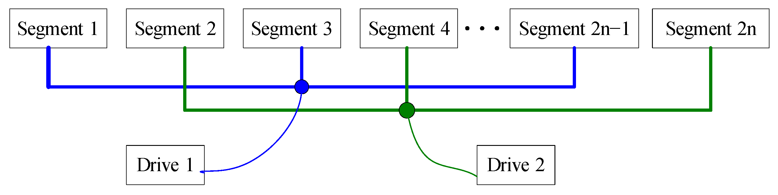
In order to improve the power supply efficiency of the WS-PMLM and reduce the expense, the stator winding usually adopts a segmented power supply method [3], that is, two drives are used in the WS-PMLM. One drive is used for the odd-numbered stator windings, and the other is used for the even-numbered stator windings. As the position of the mover changes with different stator segments, different drives are turned on, respectively, to ensure the continuous movement of the mover, such as shown in Figure 1.

This method can boost the efficiency of the drive and reduce the expense, but it makes a great challenge for the drive method, especially in the sensorless drive, because the stator of the WS-PMLM is a winding one. When the mover is between the intersegment area, it is coupled in the different stator winding at the same time, and the parameters such as inductance, flux linkage, and back-EMF of different windings vary greatly, which affects the accuracy of position and speed estimation. Therefore, accurately estimating the speed and position of the transition region between segments has become the focus of WS-PMLM sensorless driving technology.

The sensorless drive in the permanent magnet linear motor mainly has the following two categories. The first type uses external injection of a specific excitation signal to make the motor produce a certain salient pole effect, so as to establish a position estimation method according to the relationship between the motor salient pole and the position. The other type uses the mathematical model of the motor, and uses the position information contained in the mathematical model to estimate the position and speed of the mover. The first type of method mostly uses the salient pole effect of the motor, and the salient pole effect of the motor body structure needs to be considered, which is more suitable for low-speed or zero-speed occasions [8,9]. The second method uses a mathematical model of the motor to extract the position and speed signals from the motor’s flux linkage or back-EMF. In this method, when the back-EMF or flux linkage is smaller than a certain value, the estimated position and speed errors become larger, so the low-speed performance is not ideal, and it is more suitable for high-speed applications. Conventional methods are the perturbation observer method, the sliding mode observer (SMO) method [7,10,11], the extended Kalman filter method [12], and the state observer method [5,13]. The linear motor studied in this project has been applied in the high-speed field of rail transit, so the second method is more suitable for the winding segmented permanent magnet linear motor. For sensorless control at high speed, many scholars have carried out research.

Reference [14] proposes a mover position estimation method by multiple iterative search algorithm. By observing the back-EMF component of the d-axis, the mover position is obtained, and through a multiple iterative search, the best operation is selected from the estimated mover position. As the number of iterations increases, the accuracy of the mover position increases geometrically. Unlike traditional phase-locked loop (PLL), the new strategy no longer requires a proportional–integral controller.

Reference [15] presents the voltage and current model of the induction linear motor considering the dynamic end effect, and proposes a thrust model including the braking force caused by the dynamic end effect, which is realized by the Model Reference Adaptive System (MRAS) speed observer. This method enables the drive to achieve speed estimation at 0.15% of the rated speed, which greatly improves the performance of speed estimation.

In Reference [11], a high-order SMO and a second-order generalized integral PLL are proposed to realize the sensorless drive in the permanent magnet linear synchronous motor (PMLSM). A high-order SMO is used to replace the normal SMO with a low-pass filter (LPF) to avoid the phase delay caused by the LPF. It uses this technology to eliminate the chattering in the estimated back-EMF component caused by sliding mode, and realizes the sensorless control of the PMLSM with higher performance. In order to solve the chattering problem of the sliding mode observer, Reference [16] proposed an improved second-order super twisting sliding mode observer for the PMLSM. Compared to conventional first-order sliding mode observers, the estimated back-EMF does not require an extra filter, and saturation functions are used in place of sign functions to reduce further chattering.

In References [5,17,18,19], the position and speed estimation method of the WS-PMLM were presented. In order to estimate the mover position accurately, the flux linkages should be effective to be estimated in the whole stroke; for the speed estimation, a disturbance observer of the motor model was constructed to realize the speed estimation. This method can have good performance in sensorless control in the full range, and even when the mover is loaded, the speed and position can be well estimated.

From what is mentioned above, it can be concluded that if the speed and position of the mover are to be precisely obtained over the entire distance, there are two requirements: building a more suitable model for WS-PMLM, and finding an accurate and robust position and speed estimation way for the sensorless drive in the whole range.

This paper presents a sensorless drive method of the mover position and speed estimation in the WS-PMLM. Firstly, the back-EMF in the intersegment region is analyzed. Secondly, on this basis, a method for estimating the mover position by using the compound back-EMF of two adjacent stator segments is proposed. Thirdly, for fluctuations in the intersegment region produced by the speed estimation based on the PLL, the speed estimation method based on the WS-PMLM dynamics equation is studied in this paper. Finally, simulation and experiments are established to verify the effectiveness of the position and speed estimation method in the intersegment region.

2. Mathematical Model of WS-PMLM

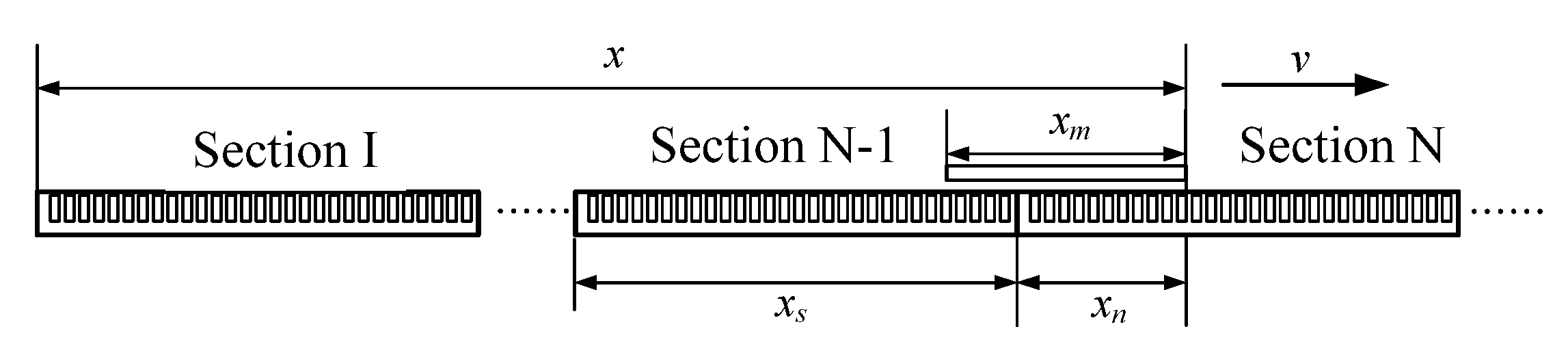
Figure 2 presents the WS-PMLM structure. Several closely connected segments comprise the primary winding, and in the length of each segment, the secondary is less than the primary. When the secondary enters or exits the n-th primary, the coupling area between the mover and different stators winding changes, so the inductance parameters and permanent magnet flux linkage parameters between the primary and secondary also vary with the position of the mover.

The WS-PMLM structure is shown in Figure 2. The primary winding is divided into several closely connected segments with equal length, and different segments in Figure 2 are marked with different subscripts. Here, x_m represents the length of the mover, x_s represents the length of each section of primary winding, and the length of the mover is less than the length of the primary winding of each section. When the mover is between the n − 1 and n-th primary windings, the coupling area between the mover and different stator windings will change, so the inductance parameters and flux linkage parameters between the primary winding and the mover will also change with the position of the mover. x_n is the distance between the mover and the n-th segment.

The inductance and flux model of the WS-PMLM is as follows:

$$L_s\left(x\right)=\left\{\begin{array}{cc}{L}_{s\sigma }+L_m·\frac{x-(n-1)x_s}{x_m}\hfill & (n-1)x_s<x\le (n-1)x_s+x_m\\ L_{s\sigma }+L_m\hfill & (n-1)x_s+x_m<x\le n{x}_s\\ L_{s\sigma }+L_m-L_m·\frac{x-n{x}_s}{x_m}\hfill & n{x}_s<x\le n{x}_s+x_m\\ L_{s\sigma }\hfill & x>n{x}_s+x_m\end{array}\right.$$

(1)

$${\psi }_f\left(x\right)=\left\{\begin{array}{cc}{\psi }_f·\frac{x-(n-1)x_s}{x_m}{e}^{j\frac{\pi }{\tau }x}\hfill & (n-1)x_s<x\le (n-1)x_s+x_m\\ {\psi }_f{e}^{\frac{j\pi }{\tau }x}\hfill & (n-1)x_s+x_m<x\le n{x}_s\\ \left({\psi }_f-{\psi }_f·\frac{x-n{x}_s}{x_m}\right)e^{j\frac{\pi }{\tau }x}\hfill & n{x}_s<x\le n{x}_s+x_m\\ 0\hfill & x>n{x}_s+x_m\end{array}\right.$$

(2)

where $n$—number of stator segments, $L_m$—magnetizing inductance, $L_{s\sigma }$—leakage inductance, ${\psi }_f$—flux amplitude, τ—pole distance (m), and x—mover position.

It can be seen from Equations (1) and (2) that the inductance and flux are functions of mover position; for simplicity, the inductance and flux can be denoted by $L_s(x)$ and ${\psi }_f(x)$, respectively. From this, the voltage equation and dynamic equation of the motor can be expressed as

$$u_s=R_s{i}_s+L_s\left(x\right)\frac{\mathrm{d}{i}_s}{\mathrm{d}t}+e$$

(3)

$$F_e=F_l+M\frac{\mathrm{d}v}{\mathrm{d}t}+Bv$$

(4)

$$F_e=\frac{3\pi }{2\tau }p\left[{\psi }_f^{n-1}\left(x\right)\cdot i_q^{n-1}+{\psi }_f^n\left(x\right)\cdot i_q^n\right]$$

(5)

where

• $u_s$—stator voltage vector in the αβ coordinate system, $u_s={\left[\begin{array}{cc}{u}_{\alpha }& u_{\beta }\end{array}\right]}^T$;
• $i_s$—stator current vector in the αβ coordinate system, $i_s={\left[\begin{array}{cc}{i}_{\alpha }& i_{\beta }\end{array}\right]}^T$;
• $e$—back-EMF vector in the αβ coordinate system, $e={\left[\begin{array}{cc}{e}_{\alpha }& e_{\beta }\end{array}\right]}^T$;
• $e=\frac{\pi v}{\tau }{\psi }_f\left(x\right){\left[\begin{array}{cc}-\sin {\theta }_r& \cos {\theta }_r\end{array}\right]}^T$;
• $v$—mover speed (m/s); ${\theta }_r$—mover theta (rad); ${\theta }_r=\pi x/\tau$; R_s—stator resistance (Ω); L_s—stator inductance; M—mover mass (kg); F_l—load thrust (N); B—friction coefficient (kg/s); F_e—electromagnetic thrust (N); p—pair pole; i_q—q-axis current; and the subscript n represents different winding segments.

3. The Mover Position Estimation of WS-PMLM Based on Disturbance Observer

Considering the back-EMF as a disturbance, a disturbance observer is constructed. Letting $\dot{e}=0$, the state equation of the motor including the back-EMF state variable is

$$\begin{array}{c}{\dot{i}}_s=A_{11}{i}_s+A_{12}e+B_1{u}_s\\ \dot{e}=0\end{array}$$

(6)

where I is unit array. $A_{11}=-\left(R_s/L_s\right)I$, $A_{12}=-\left(1/L_s\right)I$, $B_1=\left(1/L_s\right)I$.

Applying the output deviation, ${\tilde{i}}_s={\widehat{i}}_s-i_s$, the disturbance observer is built up:

$${\dot{\widehat{i}}}_s=A_{11}{\widehat{i}}_s+A_{12}\widehat{e}+B_1{u}_s+A_{11}(i_s-{\widehat{i}}_s)$$

(7)

$$\dot{\widehat{e}}=G\left({\dot{\widehat{i}}}_s-{\dot{i}}_s\right)=A_{12}G\widehat{e}+A_{11}G{i}_s+B_{1}G{u}_s-G{\dot{i}}_s$$

(8)

where G—observer feedback gain matrix, $G=g_{1}I$, $g_1$—feedback gain, and $\widehat{e}$—observed the back-EMF.

The observer error equation can be derived from Formulas (10) and (12):

$$\dot{\tilde{e}}=\dot{\widehat{e}}-\dot{e}=A_{12}G\tilde{e}=-\alpha \tilde{e}$$

(9)

where $\tilde{e}$—back-EMF error, $-\alpha$—observer pole, and $\alpha =g_1/L_s$.

To obtain the state observer stability, the error of the back-EMF adapts to the condition; in any initial condition $\tilde{e}\left(0\right)$, there is $\underset{t\to \infty }{\lim }\tilde{e}\left(t\right)=0$. Applying the Lyapunov law, and based on the back-EMF error equation, the Lyapunov function V is defined as

$$V=\frac{1}{2}{\tilde{e}}_{\alpha }^2+\frac{1}{2}{\tilde{e}}_{\beta }^2$$

(10)

where ${\tilde{e}}_{\alpha }$ and ${\tilde{e}}_{\beta }$ are the back-EMF in the αβ-axis. The derivation of the Lyapunov function is as follows:

$$\dot{V}={\tilde{e}}_{\alpha }\cdot {\dot{\tilde{e}}}_{\alpha }+{\tilde{e}}_{\beta }\cdot {\dot{\tilde{e}}}_{\beta }=-\frac{g_1}{L_s}\left({\tilde{e}}_{\alpha }^2+{\tilde{e}}_{\beta }^2\right)$$

(11)

Only when $g_1>0$ is the observer stable; then, $\dot{V}$ is negative definite. On the basis of the Lyapunov law, the disturbance observer designed is stable.

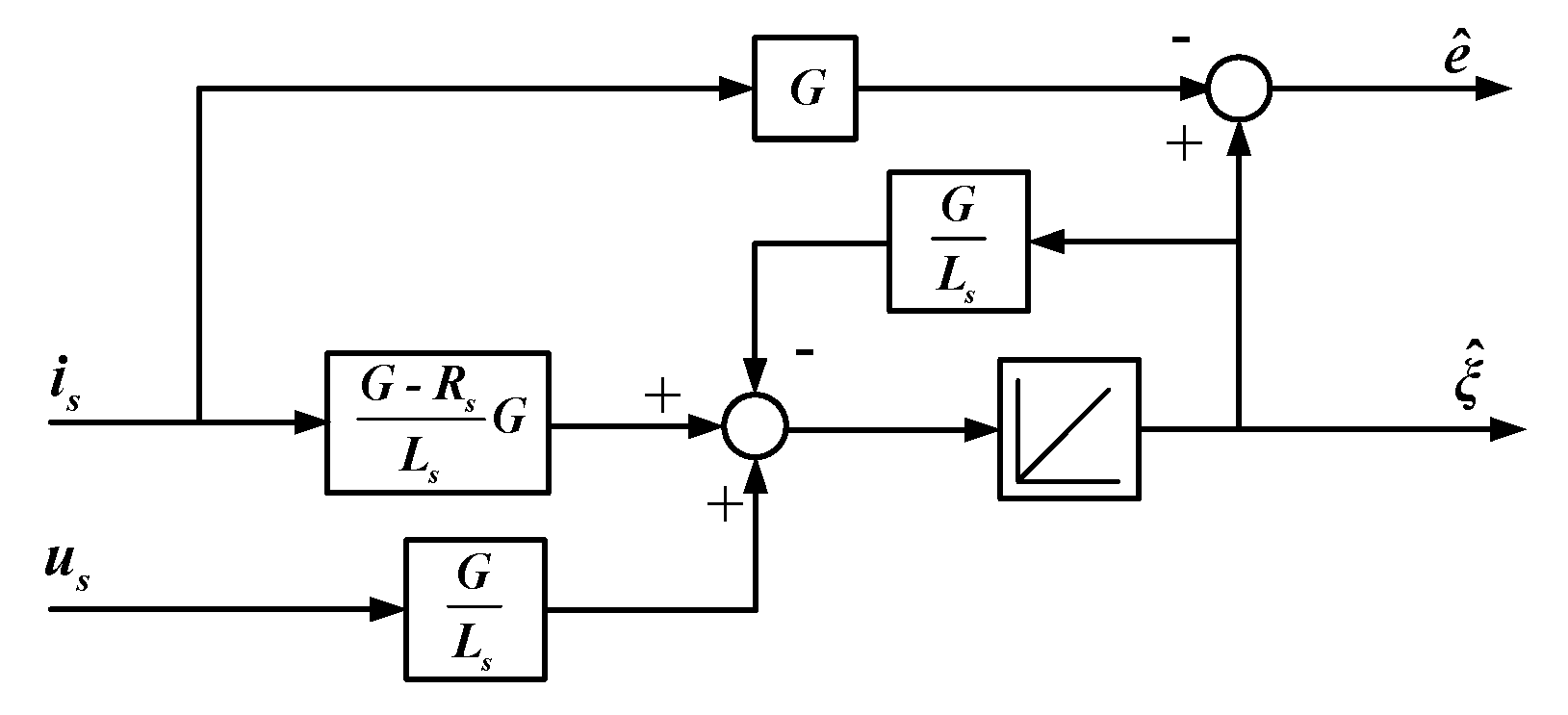
Nevertheless, the disturbance observer Equation (7) involves the derivative term of current, and the noise would be introduced in the drive. Hence, it is of necessity to optimize the observer equation and lead into new state variables:

$$\begin{array}{l}\widehat{\xi }=\widehat{e}+G{i}_s\\ \dot{\widehat{\xi }}=\dot{\widehat{e}}+G{\dot{i}}_s\end{array}$$

(12)

Substituted into Equation (7), it can be obtained that

$$\begin{array}{l}\dot{\widehat{\xi }}=A_{12}G\widehat{\xi }+B_{1}G{u}_s+G\left(A_{11}-A_{12}G\right)i_s\\ \widehat{e}=\widehat{\xi }-G{i}_s\end{array}$$

(13)

Equation (13) is the optimized disturbance observer, eliminating the derivative term of the current, and it suits application much more. It is presented in Figure 3.

4. The Mover Position Estimation between Segments

Two different stator voltage equations are shown with the mover between the n − 1 segment and the n segment.

$$\begin{array}{cc}n-1& segment\end{array}\{\begin{array}{l}{u}_1=R_s{i}_1+L_{1s}\left(x\right)\frac{\mathrm{d}{i}_1}{\mathrm{d}t}+e_1\hfill \\ e_1=\frac{\mathrm{d}{\psi }_1}{\mathrm{d}t}=j\frac{\pi v}{\tau }{\psi }_1-v\frac{{\psi }_1+{\psi }_2}{x_m}\hfill \end{array}$$

(14)

$$\begin{array}{cc}n& segment\end{array}\{\begin{array}{l}{u}_2=R_s{i}_2+L_{2s}\left(x\right)\frac{\mathrm{d}{i}_2}{\mathrm{d}t}+e_2\hfill \\ e_2=\frac{\mathrm{d}{\psi }_2}{\mathrm{d}t}=j\frac{\pi v}{\tau }{\psi }_2+v\frac{{\psi }_1+{\psi }_2}{x_m}\hfill \end{array}$$

(15)

where ${\psi }_1=\left({\psi }_f-{\psi }_f\cdot \frac{x_n}{x_m}\right)e^{j\frac{\pi }{\tau }x}$ is flux in the n − 1 segment winding, ${\psi }_2={\psi }_f\left(\frac{x_n}{x_m}\right)e^{j\frac{\pi }{\tau }x}$ is flux in the n segment winding, and $x_n=x-\left(n-1\right)x_s$.

${\psi }_1$ and ${\psi }_2$ are substituted into Equations (14) and (15), and the EMF can be expressed.

$$\begin{array}{l}{e}_1=v\frac{{\psi }_f}{x_m}\sqrt{1+{\left[\frac{\pi }{\tau }\left(x_m-x_n\right)\right]}^2}{e}^{j\left(\frac{\pi }{\tau }x+\frac{\pi }{2}-{\phi }_1\right)}\\ e_2=v\frac{{\psi }_f}{x_m}\sqrt{1+{\left(\frac{\pi }{\tau }{x}_n\right)}^2}{e}^{j\left(\frac{\pi }{\tau }x+\frac{\pi }{2}+{\phi }_2\right)}\end{array}$$

(16)

where ${\phi }_1=\arctan \left[\tau /\pi \left(x_m-x_n\right)\right]$ and ${\phi }_2=\arctan \left(\tau /\pi x_n\right)$.

From Formula (16), the back-EMF in the area between segments is different from the intrasegment. Compared with the back-EMF in the intrasegment, both the amplitude and the phase are deviated and shifted. Thus, the function of the amplitude and phase between the segments is the mover position and back-EMF, which cannot be directly and instantly applied by the disturbance observer.

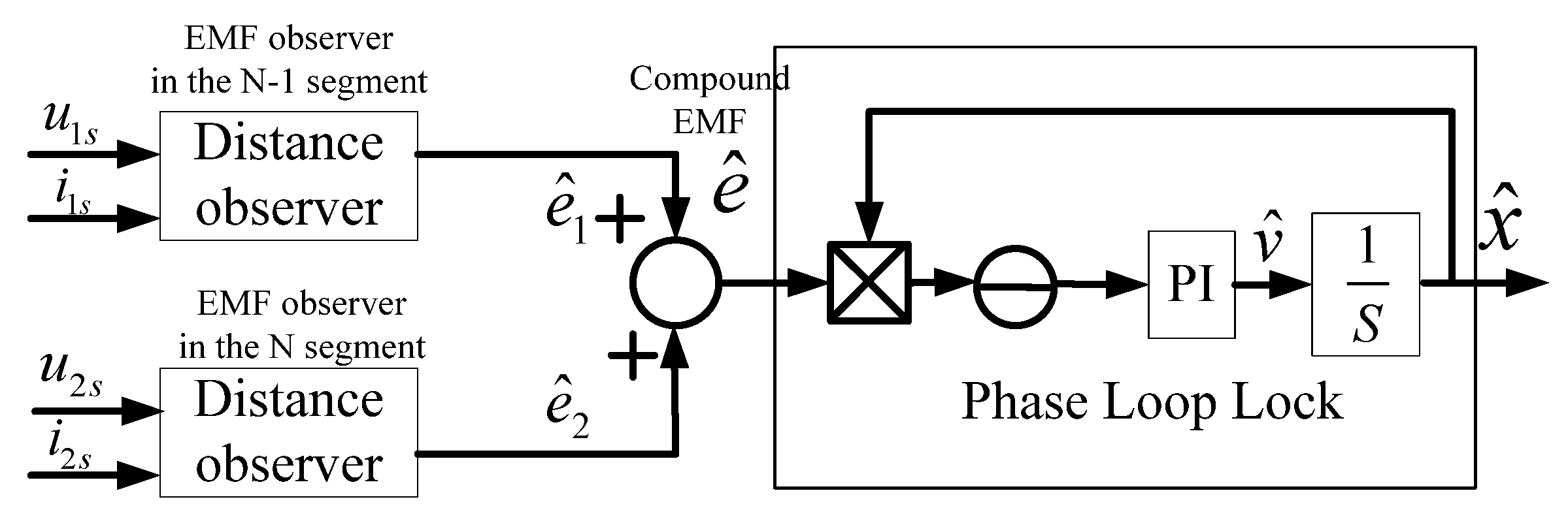
Merging the flux between different segments, the compound back-EMF can be shown as follows:

$$e=e_1+e_2=j\frac{\pi v}{\tau }\left({\psi }_1+{\psi }_2\right)=j\frac{\pi v}{\tau }\psi =\frac{\pi v}{\tau }{\psi }_f{e}^{j\left(\frac{\pi }{\tau }x+\frac{\pi }{2}\right)}$$

(17)

Although the mover is located in the different primary windings, the coupled parts of the flux are removed by the compound back-EMF. The compound back-EMF is similar to inside the segment, and the mover position between segments can be computed.

To sum up, a method for estimating the position between segments is obtained. When the mover enters the intersegment region, it is not necessary to consider the mover position on each segment, while the mover position is evaluated by the compound back-EMF. Figure 4 shows the diagram of using the compound back-EMF to achieve mover position estimation.

5. The Speed Estimation Based on Full-Order State Observer

The speed is usually estimated by the PLL method; however, the PLL is based on the motor equation, and its accuracy and stability are obviously affected by parameters such as inductance and flux linkage. For WS-PMLM in the intersegment region, the electromagnetic parameters vary greatly, and the estimated speed would have large fluctuations. This fluctuation is the disturbance in the feedback loop, which is difficult to eliminate by the controlling method, and would have a great impact on the speed loop. Therefore, this paper establishes a full-order state observer based on the motor dynamics equation to estimate the mover speed.

Considering that the load thrust changes slowly, that is, $F_l$ satisfies ${\dot{F}}_l=0$, then the dynamic equation with mover position x, mover speed v, and load thrust $F_l$ as state variables is expressed as

$${\dot{x}}_0=A_0{x}_0+B_{0}u$$

(18)

where Equation (18) is standard form. $x_0={\left[\begin{array}{ccc}x& v& F_l\end{array}\right]}^T$, $u$ is the input, $u=i_q$, $A_0=\left[\begin{array}{ccc}0& 1& 0\\ 0& -\frac{B}{M}& -\frac{1}{M}\\ 0& 0& 0\end{array}\right]$, $B_0=\left[\begin{array}{c}0\\ \frac{K_e}{M}\\ 0\end{array}\right]$.

Taking the output position as the feedback, the FSO is designed:

$$\begin{array}{l}{\dot{\widehat{x}}}_0=A_0{\widehat{x}}_0+B_{0}u+L{C}_0{x}_0-L{C}_0{\widehat{x}}_0\\ y_0=C_0{\widehat{x}}_0\\ \widehat{v}=C_1{\widehat{x}}_0\end{array}$$

(19)

where ${\widehat{x}}_0={\left[\begin{array}{ccc}\widehat{x}& \widehat{v}& {\widehat{F}}_l\end{array}\right]}^T$, $C_0={\left[\begin{array}{ccc}1& 0& 0\end{array}\right]}^T$, $C_1={\left[\begin{array}{ccc}0& 1& 0\end{array}\right]}^T$, $L={\left[\begin{array}{ccc}{l}_1& l_2& l_3\end{array}\right]}^T$, $l_1,l_2,l_3$—the observed gain, and $k_e$—the motor thrust coefficient. $K_e=\frac{3\pi }{2\tau }p{\psi }_f$.

The error equation for FSO is

$${\dot{\tilde{x}}}_0=\left(A_0-L{C}_0\right){\tilde{x}}_0$$

(20)

where ${\tilde{x}}_0=x_0-{\widehat{x}}_0$. The stability of the observer is proved in the following.

Theorem 1.

If there is a positive real symmetric matrix $P_0$, the following Equation (21) holds:

$$P_0{A}_0-Y_0{C}_0+A_0^T{P}_0-C_0^T{Y}_0^T<0$$

(21)

where $Y_0\in R^{3\times 1}$, and the feedback gain matrix satisfies $L=P_0^{-1}{Y}_0$; when the observation error exponentially approaches zero, the observer is stable.

Proof.

If Equation (21) holds, there is a matrix $Q_0>0$ and the following formula holds:

$$P_0{A}_0-Y_0{C}_0+A_0^T{P}_0-C_0^T{Y}_0^T<-Q_0<0$$

(22)

The Lyapunov function is defined as $V_0\left({\tilde{x}}_0\right)={\tilde{x}}_0^T{P}_0{\tilde{x}}_0$; $P_0$ is positive definite, so $V_0\left({\tilde{x}}_0\right)$ is positive definite, and then its derivative is

$$\begin{array}{l}{\dot{V}}_0={\tilde{x}}_0^T\left[P_0{A}_0-P_{0}L{C}_0+A_0^T{P}_0-{\left(L{C}_0\right)}^T{P}_0\right]{\tilde{x}}_0\\ {\dot{V}}_0\le -{\tilde{x}}_0{Q}_0{\tilde{x}}_0\end{array}$$

(23)

${\dot{V}}_0$ is negative definite, so ${\tilde{x}}_0$ is stable. From the state equation, the observability matrix $Q_o={\left[\begin{array}{ccc}{C}_0& C_0{A}_0& C_0{A}_0^2\end{array}\right]}^T$ is full rank, and the system is observable, so the formula is established and there is a feedback gain matrix to stabilize the observer. □

The stability is demonstrated and the feedback gain is solved by the pole placement method. We express the error equation in terms of state variables:

$$\frac{\mathrm{d}}{\mathrm{d}x}\left[\begin{array}{c}\tilde{x}\\ \tilde{v}\\ {\tilde{F}}_l\end{array}\right]=\left[\begin{array}{ccc}-l_1& 1& 0\\ -l_2& -\frac{B}{M}& -\frac{1}{M}\\ -l_3& 0& 0\end{array}\right]\left[\begin{array}{c}\tilde{x}\\ \tilde{v}\\ {\tilde{F}}_l\end{array}\right]$$

(24)

The characteristic polynomial of the error equation is

$$\begin{array}{l}\phi \left(s\right)=\det \left[sI-\left(A_0-L{C}_0\right)\right]\\ \begin{array}{cc}& \end{array}=s^3+\left(l_1+\frac{B}{M}\right)s^2+\left(l_2+\frac{B}{M}{l}_1\right)s-\frac{1}{M}{l}_3\end{array}$$

(25)

If the system expects the poles to be $p_1,p_2,p_3$, the desired characteristic polynomial is

$${\phi }^{*}\left(s\right)=\left(s-p_1\right)\left(s-p_2\right)\left(s-p_3\right)$$

(26)

The feedback gain is obtained by solving Equations (25) and (26):

$$\begin{array}{l}{l}_1=-\left(p_1+p_2+p_3+\frac{B}{M}\right)\\ l_2=p_1{p}_2+p_2{p}_3+p_1{p}_3+\left(p_1+p_2+p_3+\frac{B}{M}\right)\frac{B}{M}\\ l_3=p_1{p}_2{p}_{3}M\end{array}$$

(27)

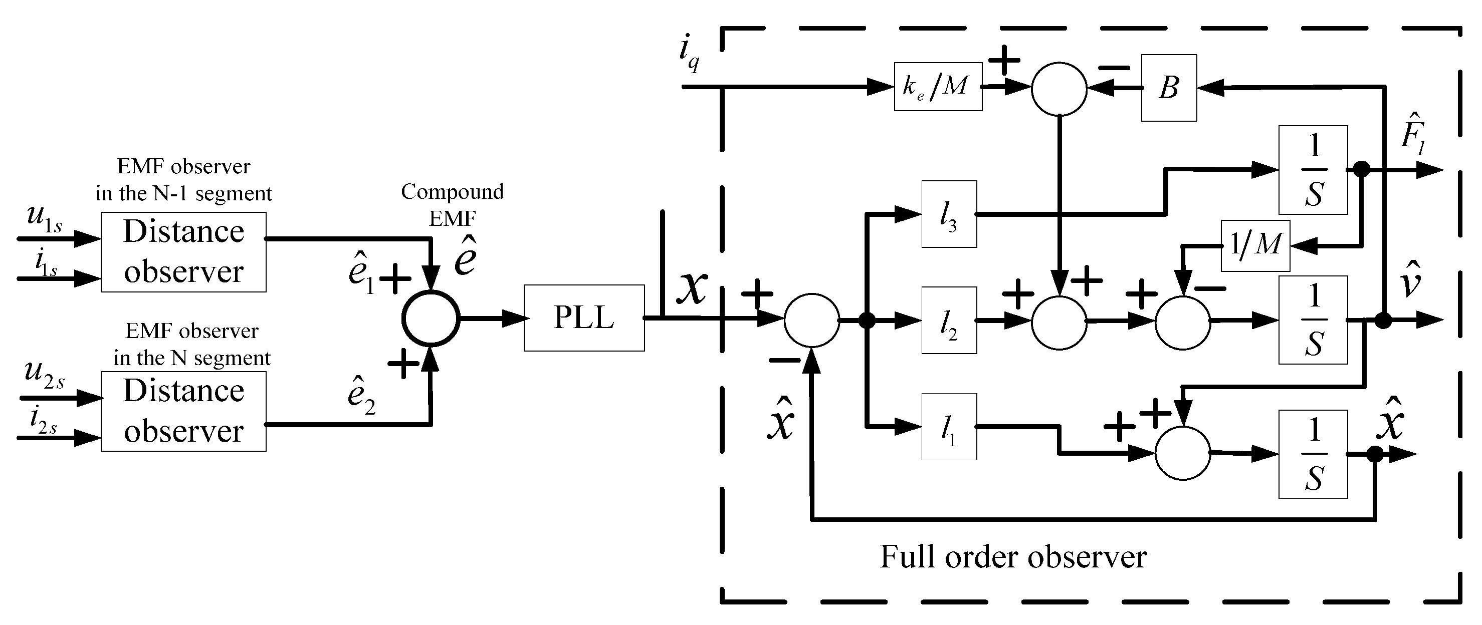
The construction of the full-order speed observer is completed and the feedback gain configuration method is obtained. The diagram of the full-order speed observer is shown in the dashed box in Figure 5.

6. Simulation

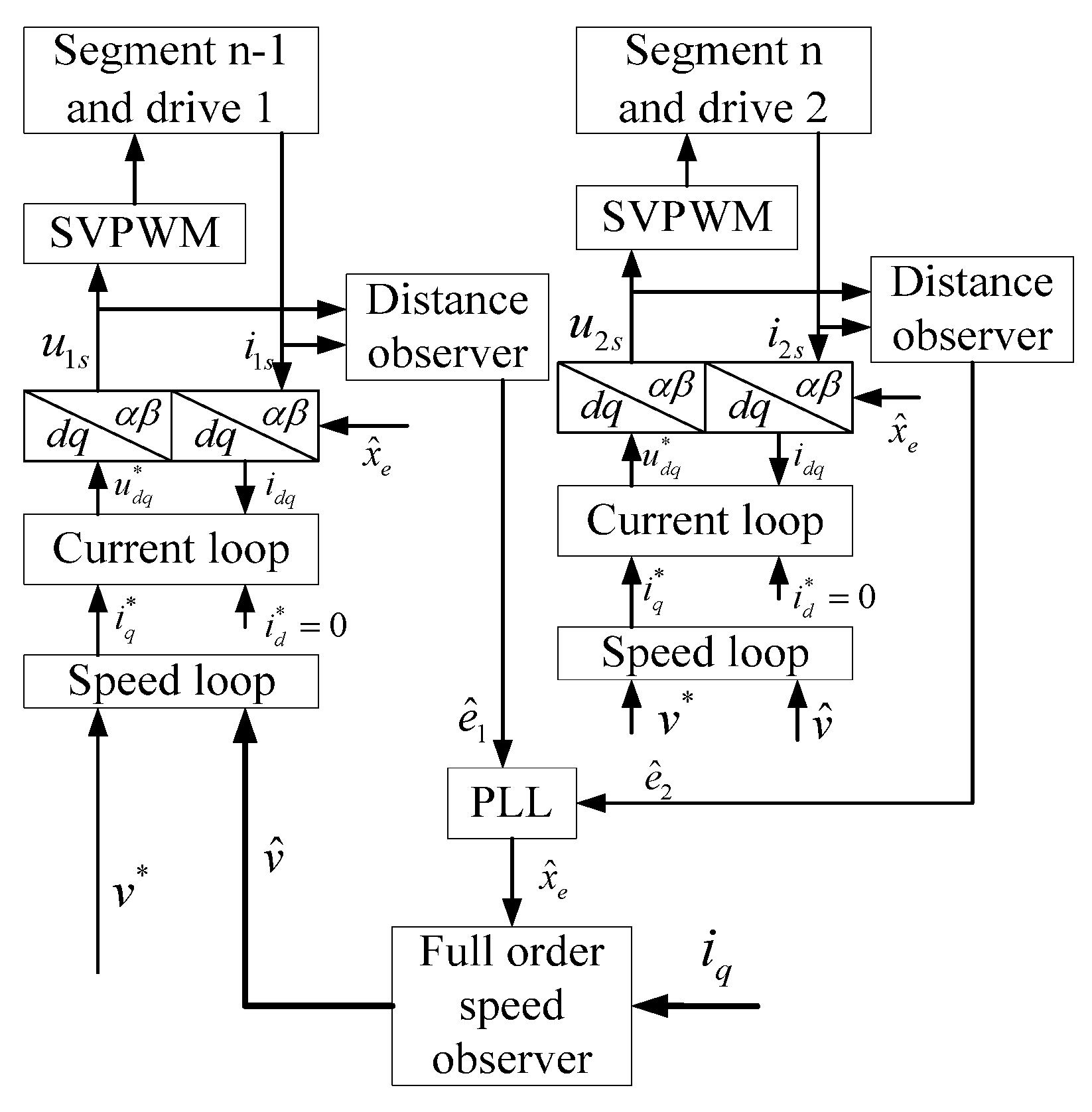
According to the above analysis, the diagram of the sensorless control of the WS-PMLM is shown in Figure 6. The WS-PMLM is driven in the segmented power supply mode. The disturbance observers I and II estimate the back-EMF of the respective winding and compound them. The FSO is used to estimate the mover speed.

Table 1. The parameters of the WS-PMLM.

Motor Data	Value
Maximum velocity	2 m/s
DC-link voltage	310 v
Ls	35 mH
Rs	1.5 Ω
Jm	0.00153 kg·m2
Force	200 N
PWM frequency	10 kHz

shows the parameters of the WS-PMLM.

The parameters of the simulation are as follows: the feedback gain g1 is set to 37.8 and the poles p1, p2, and p3 are set to −200, −200, and −800; the step signal of 1 m/s is given in the initial time; the accelerated ramp of 20 m/s² is given at the time of 0.1 s and the given speed of 3 m/s at the time of 0.2 s; the decelerated ramp of −20 m/s² is given at 0.3 s, and the constant speed of 1 m/s is given at 0.4 s. Figure 7, Figure 8 and Figure 9 show the simulation.

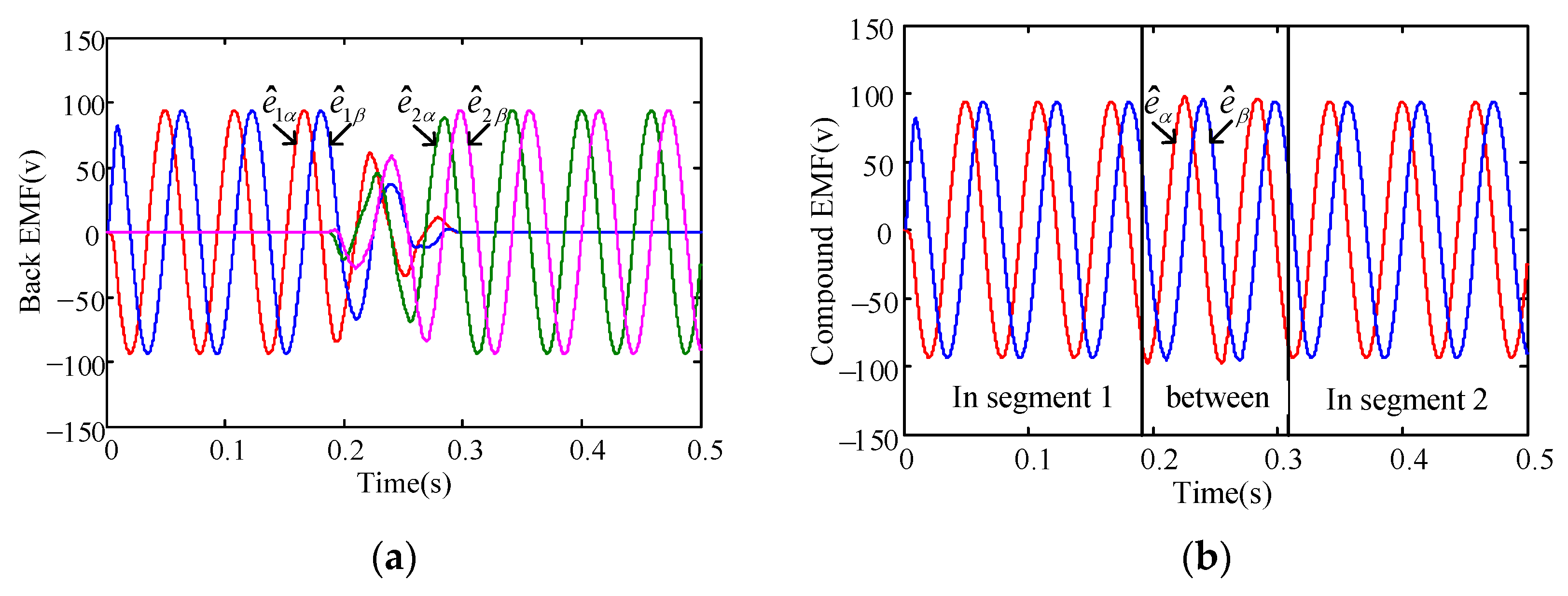
Figure 7 shows the back-EMF when the mover enters the I winding completely (0–0.18 s), in the common area of the two windings (0.18~0.32 s), and completely enters the II winding (0.32~0.5 s). When the mover is in the I winding section, the mover only induces back-EMF with the I winding section. The same situation occurs when the mover is fully in the II winding section. When the mover is located in the common area of the I and II windings, the mover induces back-EMF with the I and II winding, respectively.

Obviously, in the intersegment transition region, the amplitude and phase of the compound back-EMF do not attenuate or shift, so the compound back-EMF is more suitable for estimating the mover position in the intersegment region.

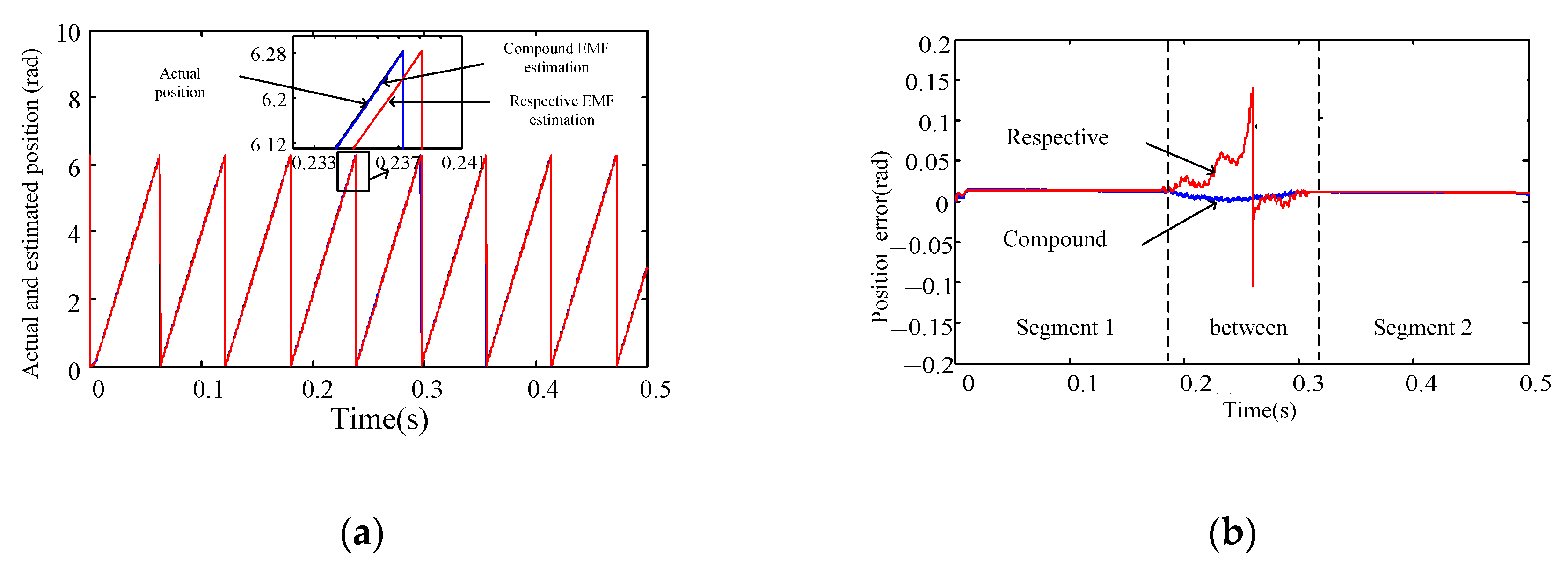
Figure 8 shows the simulation waveform. The estimated position by the respective observed back-EMF, and by the compound observed back-EMF are given under the different segment areas.

In Figure 8, the operating state of the mover is the same as in Figure 7. Obviously, using only the back-EMF generated by the mover and each segment winding to estimate the position will result in an error of up to 0.146 rad, or 8.36°. However, if the compound back-EMF method is used, the position estimation error is within 0.015 rad, which is similar to the effect of the mover in the region within the segment. Therefore, the compound back-EMF method can effectively decrease the position error.

In order to verify the estimated speed by the FSO, the simulation results of the FSO and the PLL speed estimation are compared, and the simulation results are shown in Figure 9. In order to obtain a clearer comparison of the speed estimation deviation (actual speed and estimated speed) of the two methods, the simulation results are sorted into the specific data shown in

Table 2. Comparison of speed errors between FSO and PLL.

Speed error (m/s)	0.221 s	0.236 s	0.251 s	Max
PLL	0.036	−0.035	0.039	0.039
FSO	0.009	−0.008	0.011	0.011

.

From the simulation in Figure 8 and Table 2, it can be seen that the speed error obtained by the FSO method is small, and the speed estimation error is less than 0.011 m/s, while the estimated speed error by the PLL is 0.039 m/s. It is shown that the FSO method can effectively improve the speed fluctuation between the segments, and can effectively improve the speed estimation accuracy in the WS-PMLM.

7. Experiment

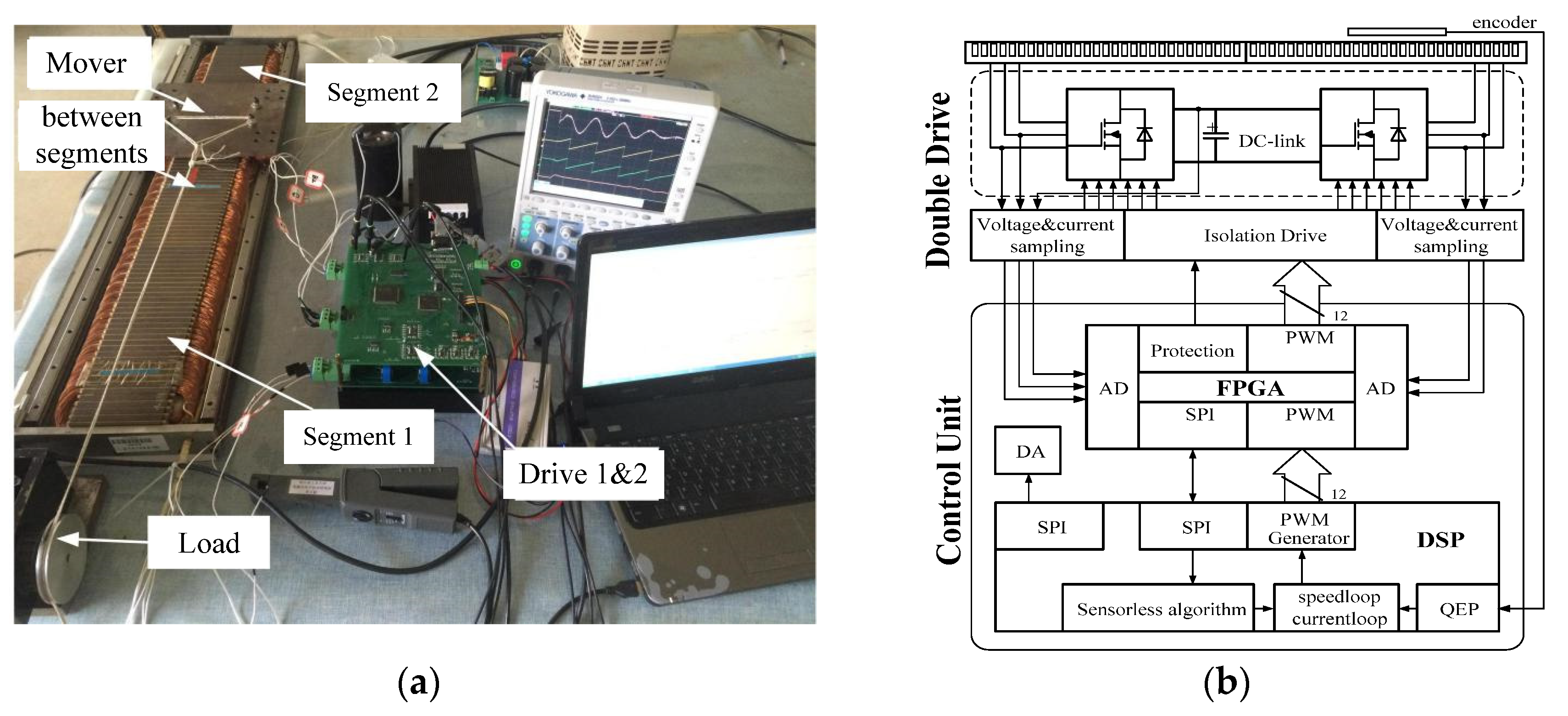
An experimental platform for the WS-PMLM was constructed so as to verify the correctness of the algorithm proposed in this paper, as shown in Figure 10. The drive part consists of two independent drive. One drive is applied for odd windings and the other is used to drive even windings. The two drives are controlled by a unified control unit. The actual position and speed of the WS-PMLM are obtained through a magnetic sensor.

In order to prove the method proposed in this paper, the DSP made by TI company, model TMS320F28335, was applied as the key algorithm control, such as the disturbance observer, sensorless, and speed and current loop, and the FPGA made by XILINX company, model XC3S400, was applied as the high-speed interface (AD, I/O). To finish making the experiment quickly, DSP was used to realize the complex control algorithm, and FPGA was only used as an interface for the real-time and fast data transmission. DSP and FPGA were connected by a high-speed data bus. In this way, DSP used its fast computing ability to implement control algorithms, and FPGA used its real-time data processing ability for fault and data processing for the drive.

The conditions in the experiment are as follows: the speed reference is 0.582 m/s, and g1 is set to 37.8. When the mover is completely inside the stator winding, the back-EMF is a magnitude of 30 v. As the mover runs, the coupling between the mover and segment I gradually goes down. Consequently the amplitude of the back-EMF progressively decreases until the mover completely exits.

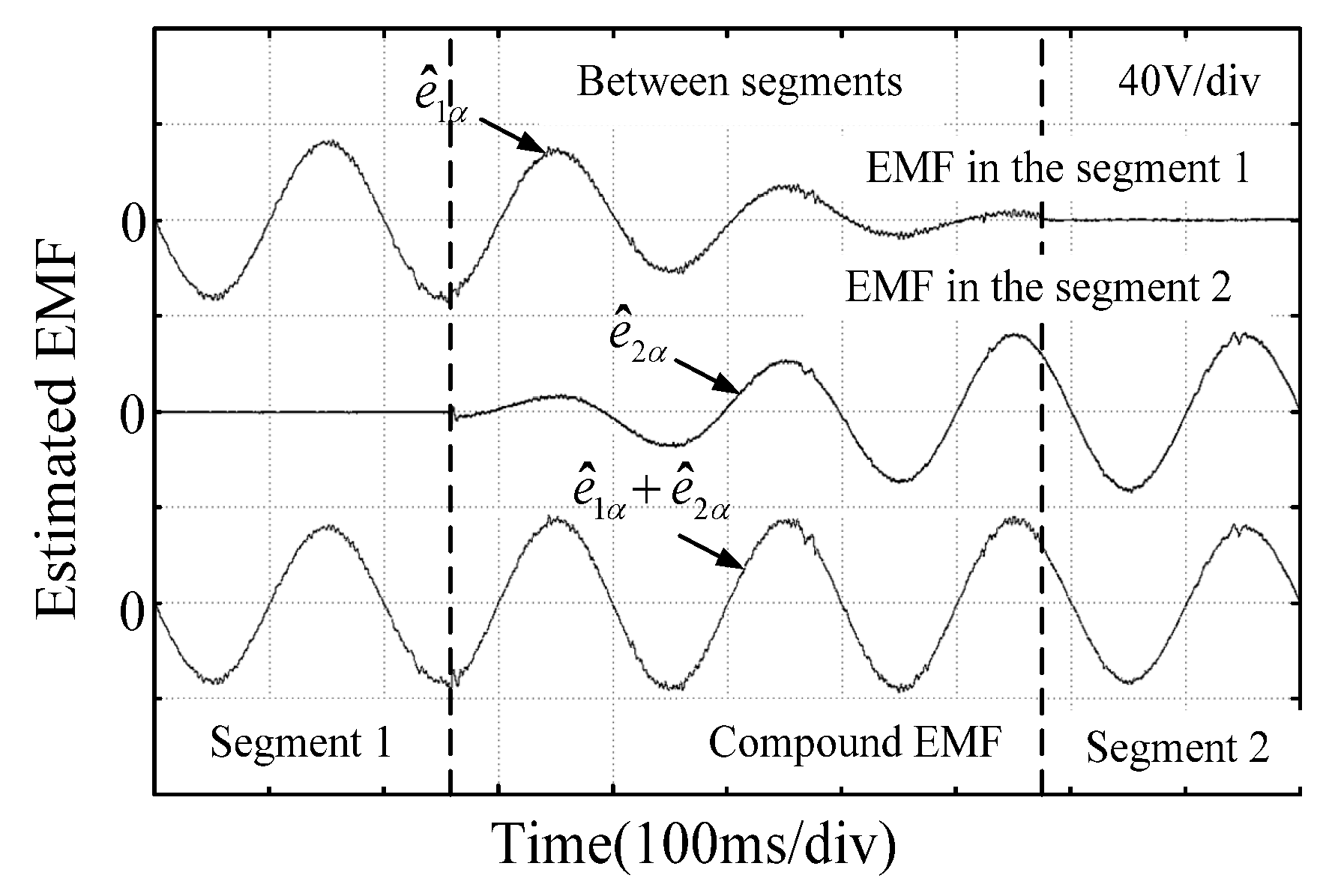
The observed back-EMF is shown in Figure 11. When the mover runs to the intersegment region, the observed back-EMF of segment I gradually decreases, the observed back-EMF of segment II gradually increases, and the compound back-EMF of segment I and segment II has the same amplitude and phase as the observed back-EMF in the segment. In other words, the compound back-EMF method has a better performance in estimating the position and speed in the intersegment region, and is more appropriate for the WS-PMLM sensorless drive.

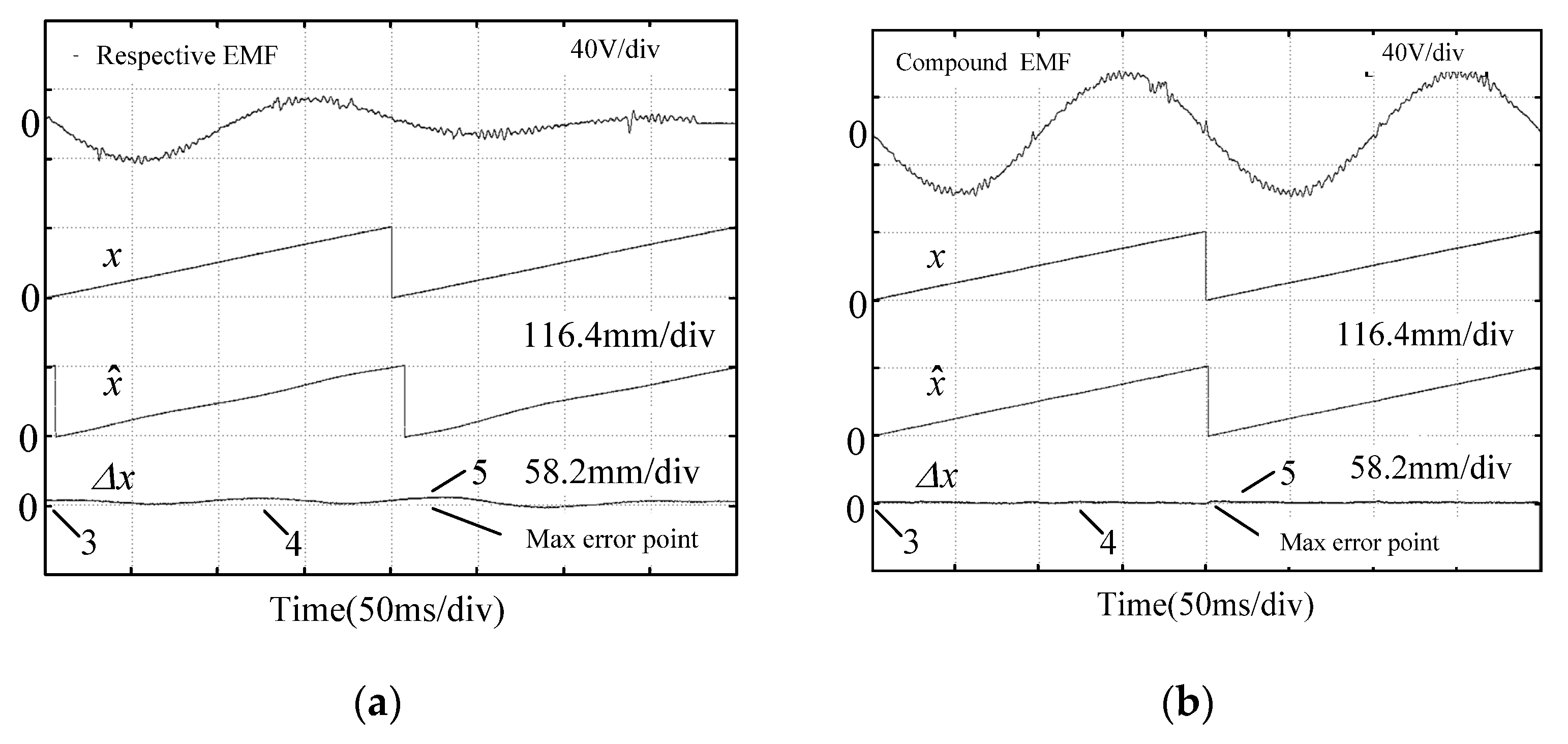
Figure 12 shows a comparison between the compound back-EMF method and the back-EMF method by only one segment winding for the position of the mover. Obviously, the position error in the compound back-EMF method is smaller.

Table 3. The error of the mover position.

Method	NO. 1 (mm)	NO. 2 (mm)	NO. 3 (mm)	NO. 4 (mm)	NO. 5 (mm)	Max (mm)
Traditional	1.18	1.15	3.20	5.82	6.54	6.54
Compound	0.87	0.98	1.04	0.89	1.16	1.55

provides detailed quantitative comparison data for the mover position errors.

In Table 3, it can be seen that the position error by the compound back-EMF method remains basically unchanged in both intrasegment and intersegment regions, with a maximum value of 1.55 mm, and the error by the respective segment back-EMF estimation method in the intersegment region rises greatly, with a maximum value of 6.54 mm. The experimental results meet the above analysis, verifying the effectiveness of the position estimation method proposed in this paper.

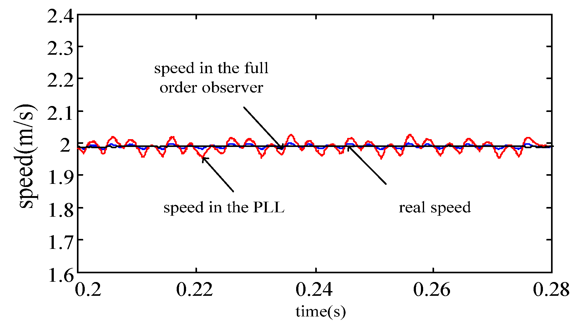
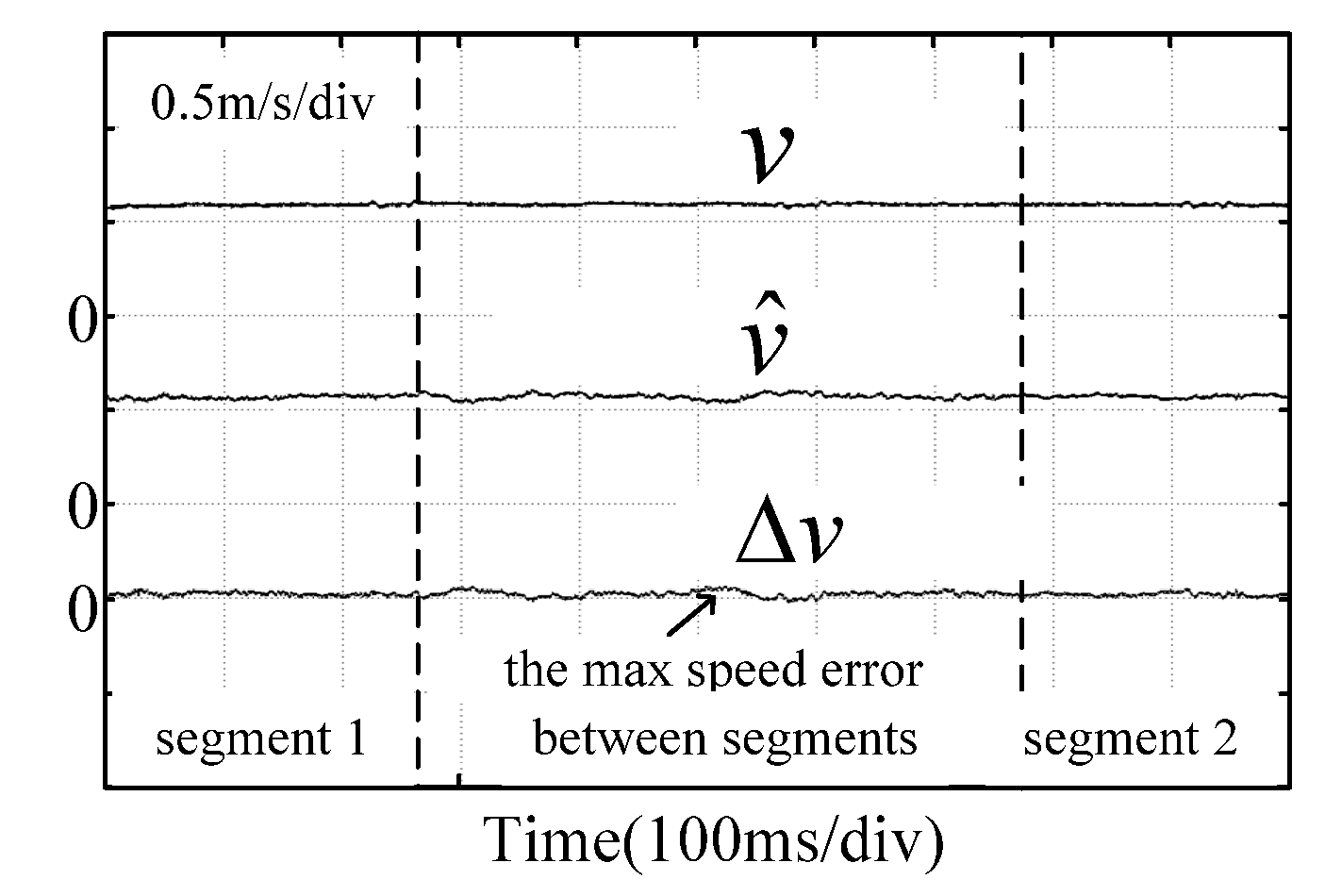
Figure 13 shows the speed estimation waveform. It can be seen that the speed error is very small, the estimated speed in the intersegment region fluctuates slightly, and the maximum speed error is less than 0.03 m/s. The proposed sensorless control method can achieve better position and speed estimation in the whole stroke.

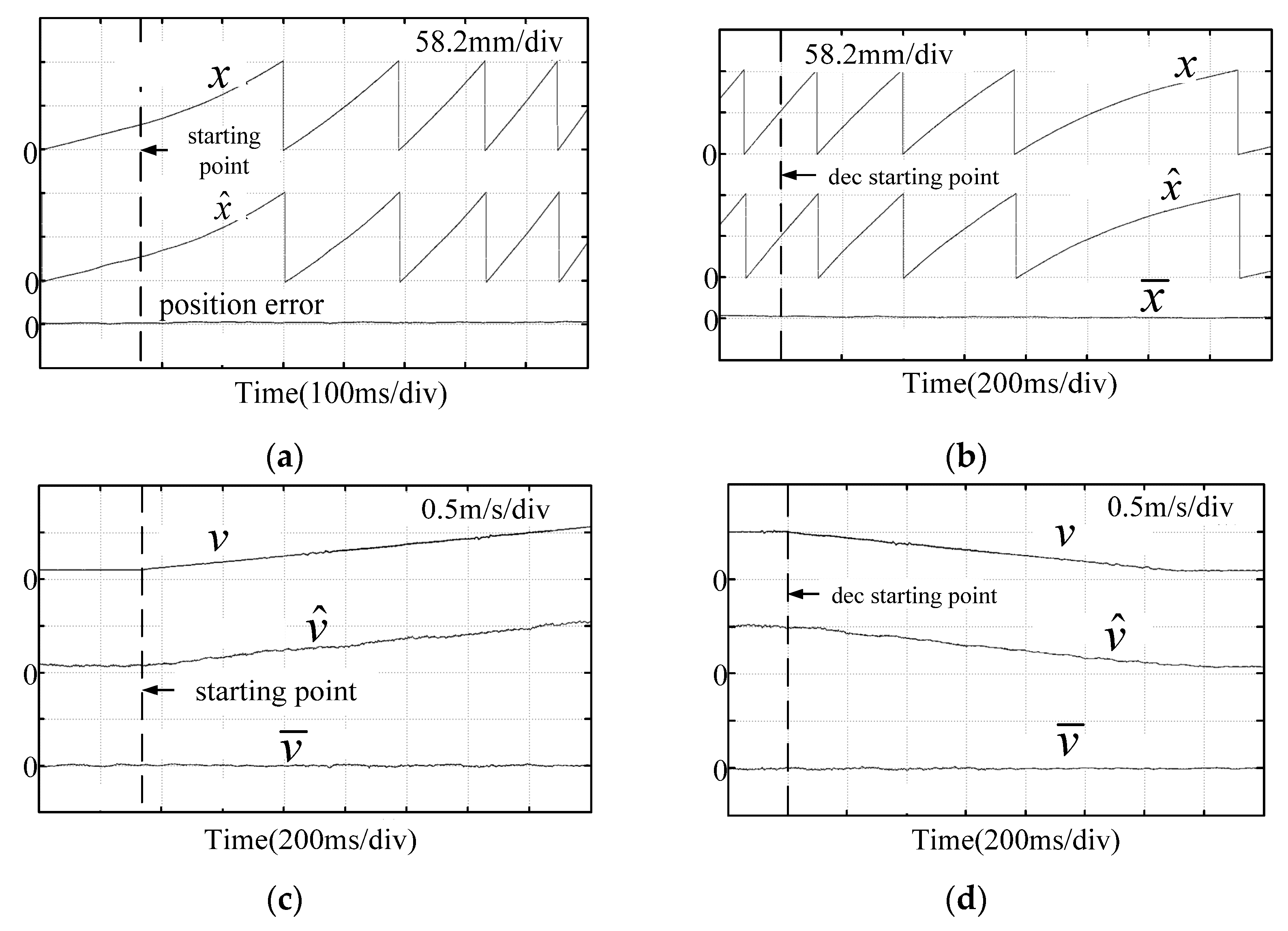
The accelerated and decelerated waveforms are shown in Figure 14; the WS-PMLM accelerates from 0.1 m/s to 0.5 m/s and decelerates from 0.5 m/s to 0.1 m/s. The position shown by the dotted line in the Figure 14 is the starting point of acceleration and deceleration. It can be seen that during the acceleration and deceleration, the estimation error of the position and speed is small, and there is no large fluctuation.

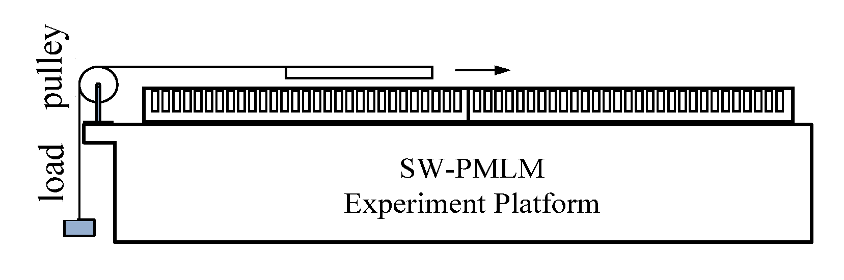
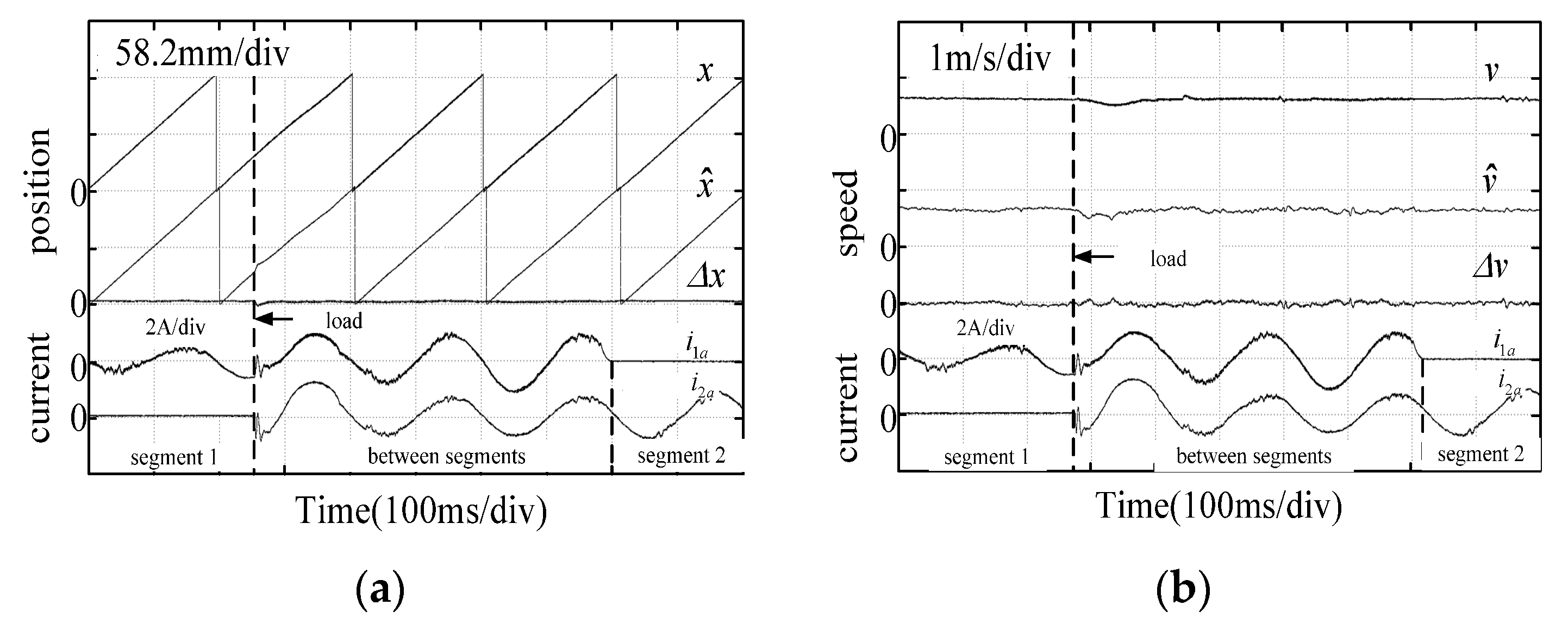
Finally, the sensorless experiment under the load was carried out. The load was applied by the pulley, as shown in Figure 15, and the load thrust was 30 N. When the WS-PMLM starts, the heavy object falls on the ground due to the long string. It has no load at this time. After the motor runs, the rope is tightened and the heavy object is lifted. This is the moment of sudden load. The phase current was monitored to characterize the change before and after loading. The speed command was 0.582 m/s. The experimental waveform is shown in Figure 16.

It can be seen from Figure 16 that sudden load has little effect on position and speed estimation. Figure 16b shows the estimated speed waveform.

8. Conclusions

This paper proposed a new method for the position estimation based on the perturbation observer by the compound back-EMF in the WS-PMLM. The FSO was obtained to increase the robustness and accuracy of the mover speed estimation in the intersegment region. Both simulation and experimental results indicate that the sensorless drive method can effectively improve the estimation accuracy of speed and position, and it has better performance on the sensorless drive in the intersegment region.