Performance Analysis of Different Optimization Algorithms for MPPT Control Techniques under Complex Partial Shading Conditions in PV Systems

Abstract

Classic algorithms show high performance in tracking the maximum power point (MPP) of photovoltaic (PV) panels under uniform irradiance and temperature conditions. However, when partial or complex partial shading conditions occur, they fail in capturing the global maximum power point (GMPP) and are trapped in one of the local maximum power points (LMPPs) leading to a loss in power. On the other hand, intelligent algorithms inspired by nature show successful performance in GMPP tracking. In this study, an MPPT system was set up in MATLAB/Simulink software consisting of six groups of serially connected PV panels, a DC-DC boost converter, and load. Using this system, the cuckoo search (CS) algorithm, the modified incremental conductivity (MIC) algorithm, the particle swarm optimization (PSO) algorithm, and the grey wolf optimization (GWO) algorithm were compared in terms of productivity, convergence speed, efficiency, and oscillation under complex shading conditions. The results showed that the GWO algorithm showed superior performance compared to the other algorithms under complex shading conditions. It was observed that GWO did not oscillate during GMPP tracking with an average convergence speed of 0.22 s and a tracking efficiency of 99%. All these evaluations show that GWO is a very fast, highly accurate, efficient, and stable MPPT method under complex partial shading conditions.

1. Introduction

The dependence on fossil fuels for energy production leads to a steady increase in carbon emissions in the atmosphere. It brings many problems, such as global warming, air pollution, and natural disasters. In addition, the increase in global energy demand is constantly depleting oil and natural gas reserves. For these reasons, the issue of global warming and energy policies has recently become a controversial issue around the world. Every day, more and more countries are trying to reduce their greenhouse gas emissions and are turning to alternative energy production sources [1]. Renewable energy generation sources are more suitable options as they are clean, inexhaustible, and reliable. Preferring these resources can reduce fossil fuel imports, environmental pollution, and global warming problems. It also enables society to secure energy independence.

Recently, photovoltaic (PV) energy has come to the fore among renewable energy generation resources. Some of its advantages are that it is harmless, beneficial, and environmentally friendly. Once PV energy systems are built, they generate electricity from sunlight without causing greenhouse gas emissions. They have an average lifespan of 20–25 years, and during this time they can obtain much more electrical energy than is required. They can also be built on rooftops, in the desert, and in rural areas. They require little maintenance and do not create air and noise pollution [2,3].

PV energy systems have some disadvantages as well as all these advantages. These are low energy efficiency, high production cost, and high initial investment cost. The characteristic curve of the PV panel is not linear. In other words, it depends on the irradiation level and temperature factors. Therefore, the value of power at the maximum power point in a PV energy system varies depending on weather conditions. To eliminate all these negativities and increase efficiency, tracking the maximum power point has been considered as a way forward [4]. The MPP defines the maximum possible power that can be produced from a PV panel. Maximum power point tracking (MPPT) is desired to operate the panel at the point where the highest possible power will be provided. If the operating point is close to the MPP, low power losses are observed, and if it is distant from it, high-power losses are observed. Therefore, proper tracking of the MPP in changing weather conditions is essential to ensure maximum power is drawn from the PV panels [5].

In modern renewable PV energy systems, this process is provided by MPPT algorithms. In other words, a DC–DC converter is used that controls the duty cycle value depending on the voltage and current values obtained from the panel. In addition, through the MPPT system, the operating point can be adjusted to produce the highest maximum power [6]. Therefore, considering this information, the MPPT system can be defined as an electronic system designed to produce maximum power by changing the duty cycle of PV panels [7]. Numerous methods have been developed and studies have been conducted on maximum power point tracking in the last decade in the literature. These methods were compared in terms of criteria such as convergence speed, tracking accuracy, efficiency, complexity, and cost [8]. A PV panel shows only one MPP when exposed to constant irradiation and using any of the traditional MPPT methods this point can be easily tracked. Examples of classic MPPT methods include perturbed and observed (P&O) [9], incremental conductivity (IC) [10], open-circuit voltage [11], and short-circuit current [12]. Research on these has generally focused on the speed of convergence to MPP and high tracking accuracy. However, the panels may not receive homogeneous irradiation at all hours of the day due to many environmental factors, such as moving clouds, shade from buildings and trees, and dusting. When partial shading conditions occur, more than one maximum power point occurs in the PV curve. In this case, classic methods will fail to track the appropriate GMPP [13].

Many intelligent methods have been presented, developed, and published to address the multi-MPP issue in partial shading. Particle swarm optimization (PSO) [14], the cuckoo search algorithm (CSA) [15], grey wolf optimization (GWO) [16], the firefly algorithm (FA) [17], artificial bee colony (ABC) [18], ant colony (AC) [19], the bat algorithm (BA) [20], whale optimization (WO) [21], the butterfly optimization algorithm (BOA) [22], the salp swarm algorithm (SSA) [23], fuzzy logic (FL) [24], the genetic algorithm (GA) [25], artificial neural networks (ANN) [26], Harris hawks optimization (HHO) [27], and the Jaya algorithm (JA) [28] are some of these methods. In addition, these methods have been used and developed in a modified or hybrid manner. Examples of these include variable step size P&O [29], modified incremental conductivity (MIC) [30], modified PSO (M-PSO) [31], modified firefly algorithm (M-FA) [32], ANN with GA [33], P&O with PSO [34], modified P&O with ANN [35], and P&O with the bat algorithm [36].

As a result of the examination of the studies in the literature, it was observed that these methods were operated under two types of conditions. The first are studies in which constant irradiation has the same effect throughout the entire system. The second are studies where partial shading conditions occur in a certain part of the system. In this study, complex partial shading, which is a more difficult condition for MPPT, is discussed. In MATLAB/Simulink, a system consisting of six series-connected PV panels, one DC–DC boost converter, and one load was designed. CS, GWO, MIC, and PSO algorithms were used in the designed system. These algorithms were run in five different uniform and complex partial shading conditions. The algorithms were evaluated and compared in terms of convergence speed, efficiency, oscillation, and productivity criteria.

2. Materials and Methods

2.1. Renewable PV Energy Systems

The concept of photovoltaic energy refers to the process of obtaining electrical energy as a result of the absorption of sunlight falling on solar panels. This concept was first introduced by Alexandre Edmond Becquerel in 1839. Becquerel expressed this concept by observing that when light falls on a solid electrode placed in a liquid electrolyte solution, a voltage is created at the ends of the electrode. PV energy systems can be designed in many ways for various applications and requirements. A block diagram describing the structure of a renewable PV energy system is given in Figure 1.

Renewable energy systems include PV panels, batteries, inverters, charge regulators, and electronic circuits. The direct current (DC) obtained by falling sunlight on the solar panels is provided by DC–DC converters in various topologies in the system. The resulting DC is converted into alternating current (AC) with the help of inverters and is prepared for use. PV energy systems are mostly categorized into three different groups: off-grid, on-grid, and hybrid.

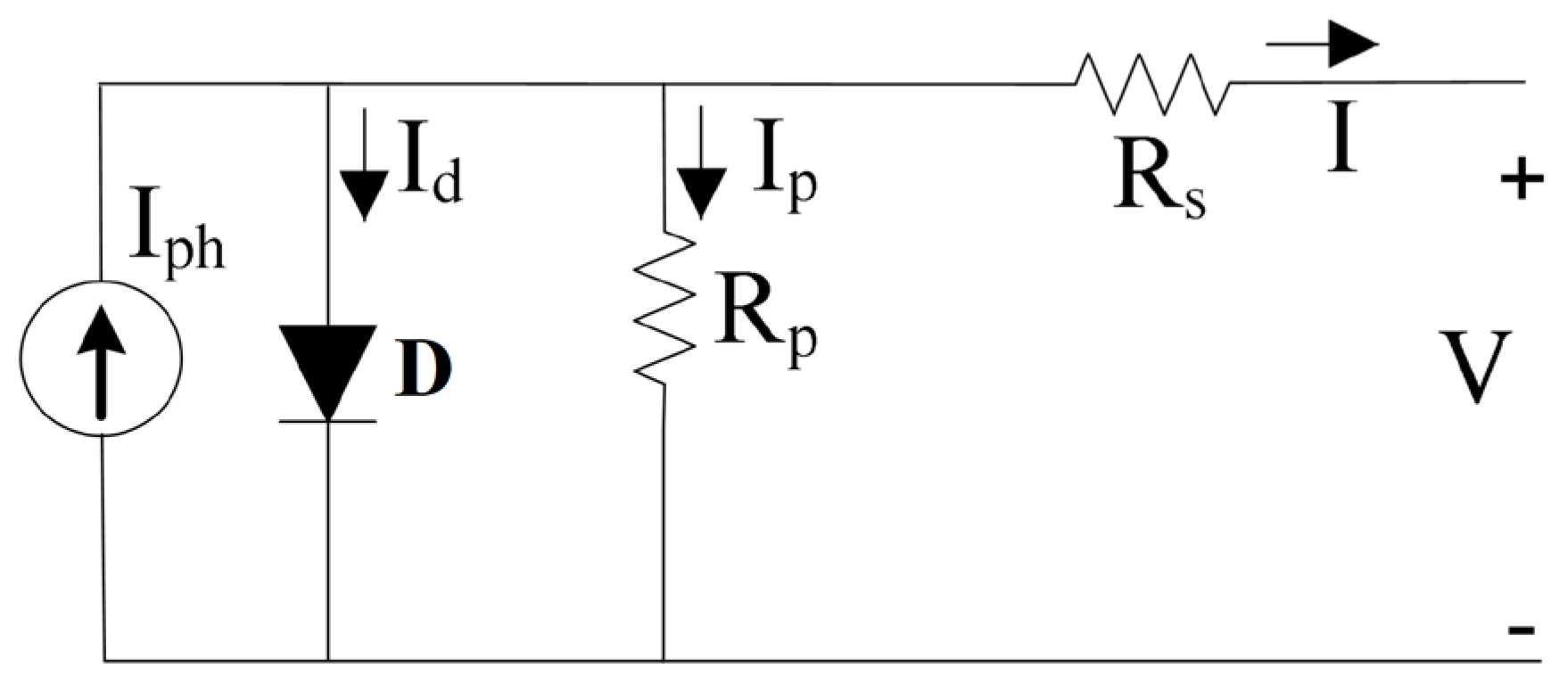
2.1.1. PV Cell Modelling

For PV cells, the single diode equivalent circuit model is the preferred notation due to its simplicity. This model consists of a current source (I_ph), a diode, a resistor in parallel (R_p), and a resistor in series (R_s) [38]. Figure 2 shows the electrical equivalent circuit model of the PV cell. The output current of the PV cell is given in Equations (1)–(3).

$$\mathrm{I}={\mathrm{I}}_{\mathrm{ph}}-{\mathrm{I}}_{\mathrm{d}}$$

(1)

$$\mathrm{I}={\mathrm{I}}_{\mathrm{ph}}-{\mathrm{I}}_0\left[\exp \left(\frac{\mathrm{V}+\mathrm{I}{\mathrm{R}}_{\mathrm{s}}}{\mathrm{a}}\right)-1\right]-\frac{\mathrm{V}+\mathrm{I}{\mathrm{R}}_{\mathrm{s}}}{{\mathrm{R}}_{\mathrm{p}}}$$

(2)

$$\mathrm{a}=\frac{{\mathrm{N}}_{\mathrm{s}}\mathrm{nkT}}{\mathrm{q}}$$

(3)

In the above equations, I₀ represents the reverse saturation current of the diode, an ideal factor, N_s is the number of cells connected in series, n is the diode ideal constant, k is the Boltzmann constant, T is the cell temperature, and q is the electron charge. The current obtained by the effect of the light falling on the PV cell is given in Equation (4).

$${\mathrm{I}}_{\mathrm{ph}}=\left({\mathrm{I}}_{\mathrm{ph},\mathrm{n}}+{\mathrm{K}}_1\left(\mathrm{T}-{\mathrm{T}}_{\mathrm{n}}\right)\right)\frac{\mathrm{G}}{{\mathrm{G}}_{\mathrm{n}}}$$

(4)

In the above, I_ph indicates the current obtained under standard test conditions. T_n refers to the rated temperature. It shows the G irradiation value and the G_n nominal irradiation value (W/m²). The saturation current of the diode is expressed in Equation (5).

$${\mathrm{I}}_0=\frac{{\mathrm{I}}_{\mathrm{S}\mathrm{C},\mathrm{n}}+{\mathrm{K}}_1\left(\mathrm{T}-{\mathrm{T}}_{\mathrm{n}}\right)}{\exp \left(\frac{{\mathrm{V}}_{\mathrm{O}\mathrm{C},\mathrm{n}}+{\mathrm{K}}_{\mathrm{V}}\left(\mathrm{T}-{\mathrm{T}}_{\mathrm{n}}\right)}{\mathrm{a}}\right)-1}$$

(5)

In the above equation, I_SC,n represents the rated short-circuit current, V_OC,n represents the rated open-circuit voltage, K₁ is the current coefficient, and K_V is the voltage coefficient [39]. In this study, six series-connected TATA power solar system TP250MBZ PV 250 W polycrystalline modules were used in the system design. The solar PV module parameters are given in

Table 1. TATA power solar system TP250MBZ module parameters.

Power at STC (W)	250	Vmp: Voltage at Max Power (V)	30
Power at PTC (W)	222.7	Imp: Current at Max Power (A)	8.3
Power Density at STC (W/m2)	151.515	Voc: Open Circuit Voltage (V)	36.8
Power Density at PTC (W/m2)	134.97	Isc: Short Circuit Current (A)	8.83

.

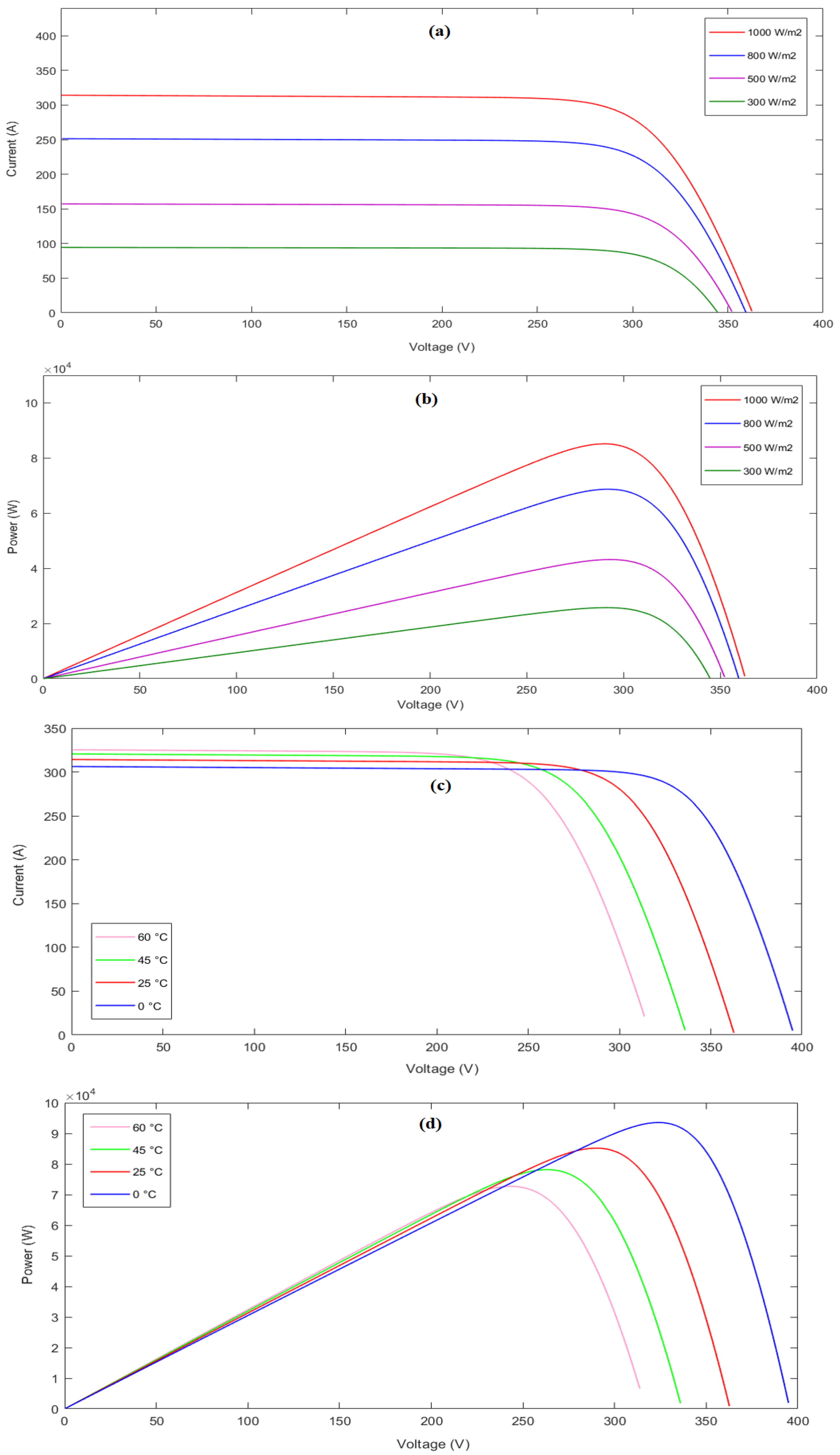
2.1.2. PV Energy Systems under Different Irradiation and Temperature Conditions

The two most important factors that determine the maximum power that can be obtained in PV energy systems are the solar irradiation and the temperature. The power obtained from the PV panel is calculated by multiplying the panel voltage and the current. There is a standard test condition for PV energy systems. This condition is used to assess the efficiency of PV energy systems. In the datasheets of PV panels, there are generally values in these standard test conditions. In the power–voltage characteristic curve, there is a maximum power generated for a given voltage and current value. Standard test conditions are defined as 1000 W/m² irradiance and 25 °C temperature [40]. However, these conditions may not be met continuously. Changes in irradiation and temperature also affect the output current and voltage of the PV panel [41]. Figure 3 shows the effect of the PV panel at different irradiance and temperature values on the current–voltage and power–voltage characteristic curves.

In Figure 3, it is seen that increase in the irradiance while the PV panel is under constant temperature increases the output current. In this case, the maximum output power of the PV system is directly affected by change in the current value. As a result, the increase in irradiation causes the output power to increase as well. When the figures are examined, it is seen that increase in temperature while the PV panel is under constant radiation reduces the output voltage. In this case, the maximum output power of the PV system is directly affected by decrease in the voltage value. As a result, increase in temperature causes the output power to decrease.

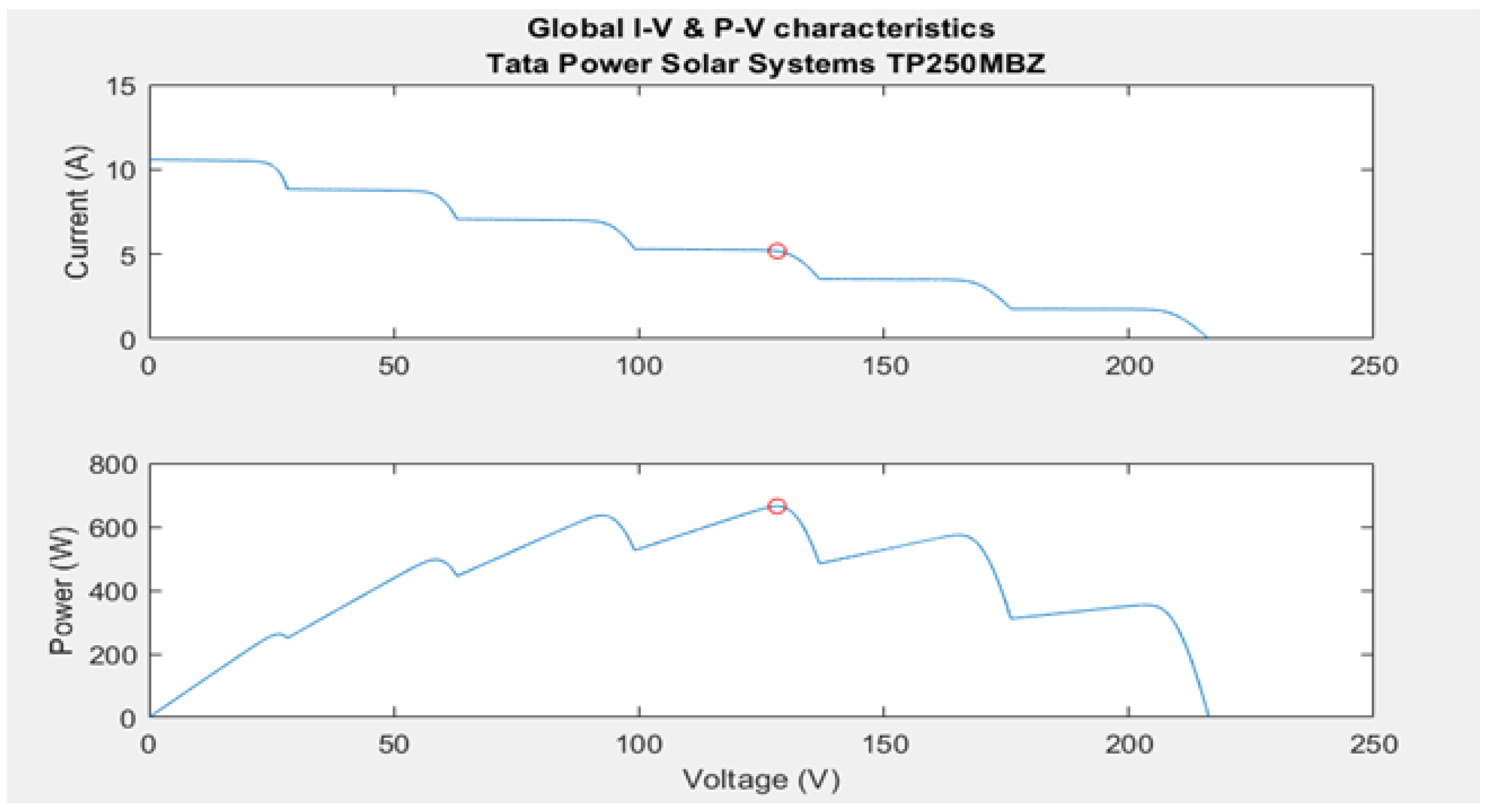
2.1.3. The Effect of Partial Shading Conditions on PV Energy Systems

The PV panel achieves only one MPP under standard test conditions. It is generally accepted that all panels operate in the same weather conditions in most MPPT methods. However, this may not always be true. One of the important variables affecting the efficiency of PV panels is shading. The efficiency of the power value to be produced from a PV panel is very sensitive to the shading conditions. The power loss varies depending on two factors. These are the type of shading and the area of the shaded part [42]. Panels may operate under partial shading conditions due to environmental factors, such as the shadows of clouds, tall buildings, tree branches, or other objects moving on the PV panels. In such a case, solar panels with less irradiation on them will receive less current than other panels. The reduced current of the panels will cause a decrease in the output power value. In this case, the high current obtained in the panels that are not under shading damages the panels operating under partial shading. To prevent this harm, bypass diodes connected in parallel are added to all PV panels. Thus, the high current to be obtained will proceed through the bypass diode circuit and prevent damage to the PV panels operating under partial shading conditions [43]. In the power–voltage characteristic curve of a PV system operating under partial shading conditions, peaks occur as much as different irradiance values. Only one of these peaks has the highest output power and is called the GMPP. Other points are called LMPPs. Partial shading does not only cause the output power and voltage values of PV systems to decrease. At the same time, it causes the formation of hot spots in the PV panels.

As a result, the physical structures of the PV panels due to overheating are damaged. To prevent such undesirable situations, bypass diodes are added to all PV panels in parallel. Bypass-connected diodes are passive in normal operation, where they are not subject to partial shading. That is, they do not affect the system. However, when exposed to partial shading, diode circuits connected to the bypass in the PV panels with shading become active and take precautions against the hot-spot event. In addition to all these benefits of bypassing connected diodes, they also have different problems. One of these problems is the inability to produce power or energy on the PV panel, which is exposed to partial shading where the bypass-connected diode circuit operates. Thus, the maximum power value decreases. Due to the presence of bypass-connected diodes, peaks occur in the power–voltage characteristic curve of the PV energy system as often as the number of different irradiations. As a result, the system becomes complex [44]. The power–voltage and current–voltage characteristic curves of the PV panel obtained for the complex shading condition are given in Figure 4.

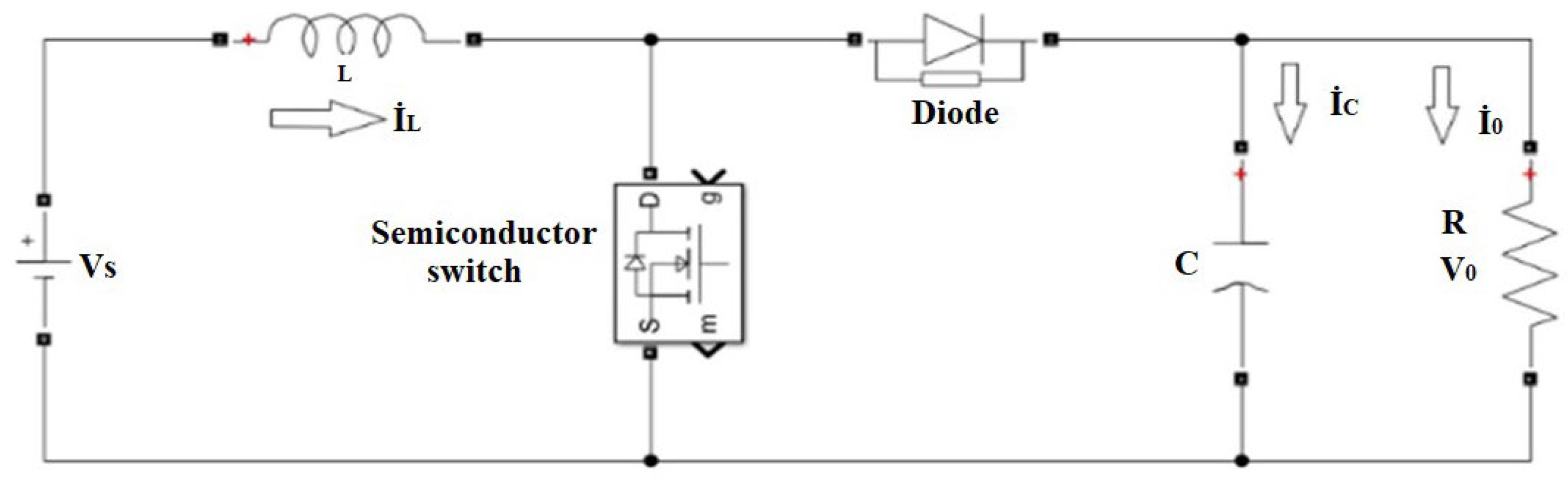
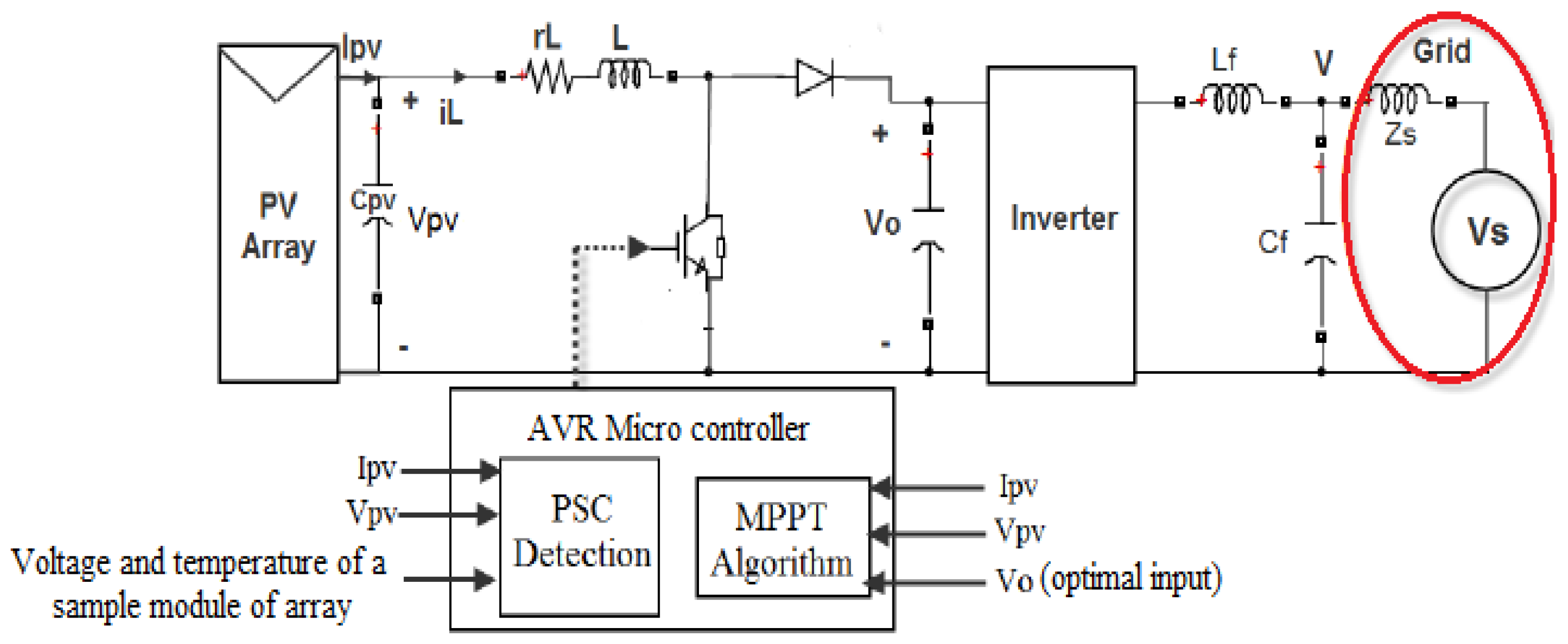
2.1.4. DC–DC Boost Converter

DC–DC converters are electronic circuits that are widely used to convert unregulated DC input power to regulated DC output power at different voltage and current levels [45]. They are used to adjust and control the varying output power of solar panels to ensure that the operating point is always at MPPT. This can be accomplished using one of the MPPT techniques to change the duty cycle (D) applied to drive the converter [46]. The DC–DC boost converter is one of the most widely used topologies among power electronics circuits. It is used in applications where the output voltage is required to be higher than the input voltage. The desired output voltage can be obtained by changing the duty cycle applied to the switch under a fixed frequency [47]. The relationship between D, the input voltage V_in and the output voltage V₀ of the boost converter is shown in Equation (6). The boost converter circuit is shown in Figure 5.

$$\frac{{\mathrm{V}}_0}{{\mathrm{V}}_{\mathrm{i}\mathrm{n}}}=\frac{1}{1-\mathrm{D}}$$

(6)

Figure 6 shows a two-stage grid-connected system. The purpose of the DC–DC boost converter in early stages of the process is to control the voltage of the PV array so that electricity may be gathered. An inverter controls the DC–DC converter’s output voltage while also producing the AC voltage needed for connecting the solar system with the grid during the second stage. Coupling among the two stages is minor due to the presence of a DC link capacitor among the boost converter as well as the inverter, allowing them to be investigated independently.

When using a boost converter to regulate a PV array, either an open or closed loop can be utilized. When operating at constant current and low irradiance, a photovoltaic array’s dynamic resistance is at its lowest. The stability and dynamic response are terrible. A single-loop PI voltage controller cannot close-loop control the array voltage because the system’s dynamic response depends on the operating point and environmental conditions. Inner control requires a boost converter inductor current loop. Two PI controllers and a costly current sensor are required for this solution. It is most common to control a boost converter in an open loop. There is no feedback in this approach; the proper input voltage is obtained by comparing the input and output voltages of the converter. This method eliminates the need for an expensive current sensor by not measuring the inductor current. The system response may result in more transient and steady-state errors than the closed-loop method. In PV MPPT, sampling time is a key parameter. Before applying a new command voltage V_in^ref to the converter after the system’s transient response has stabilized, a voltage and current sample must be taken from the array. So, sampling must take longer than the settling time.

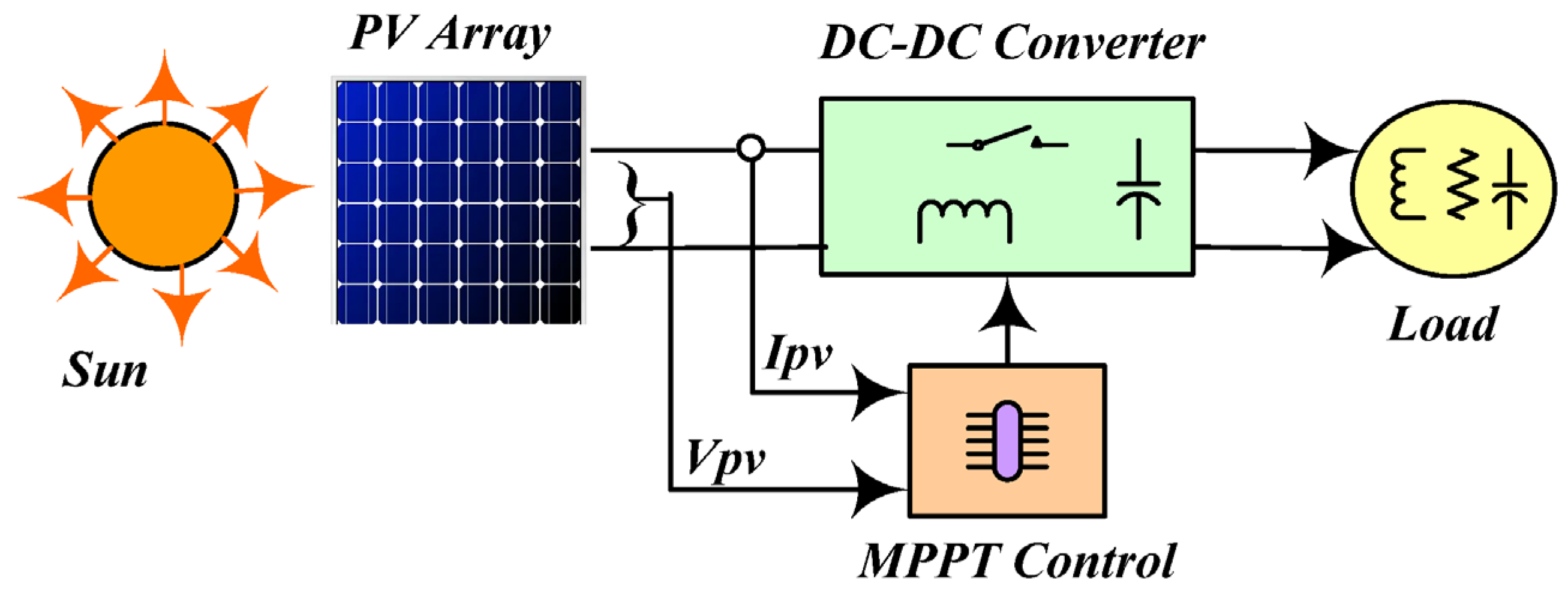
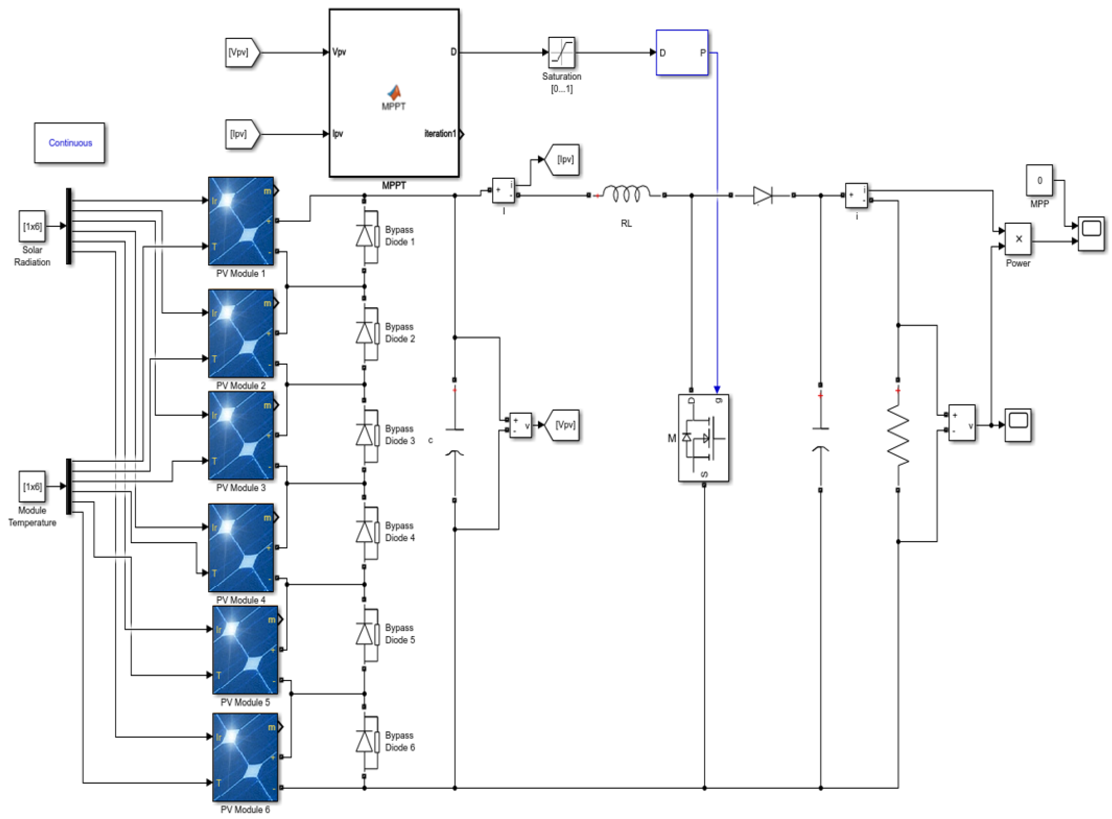
2.1.5. System Design

In this section, first, a PV system is designed in MATLAB-Simulink software (version R2022b). This system was tested under uniform and complex partial shading conditions for five different situations. The current–voltage (I-V) and power–voltage (P-V) characteristic curves were obtained and investigated for five different cases. Then, they were added to the created system, respectively, the CSA, GWO, MIC, and PSO algorithms from the MPPT methods. Each algorithm was started in five different uniform and complex partial shading conditions, respectively, and their graphics were obtained. The algorithms were compared in terms of convergence speed, efficiency, oscillation, and power criteria. The MATLAB-Simulink software image of the designed system is given in Figure 7.

2.2. Maximum Power Point Tracking

The initial investment cost of PV energy systems is high. In addition, it is intended to generate electrical energy with high efficiency from these systems. Therefore, maximum power point tracking methods are needed. Various methods are being developed to obtain maximum power from PV energy systems. Electronic tracking is one of these developed methods. This method aims to find the operating point at which the power of the system is maximal. Many algorithms are used for this purpose. These algorithms try to maintain or further improve the MPP value with various scenarios in its structure. This method is called maximum power point tracking. Tracking the MPP value with an algorithm used in the system will not require redundant materials and maintenance costs. Therefore, it is the most logical solution to use MPPT algorithms to increase the efficiency of the PV panel. Ongoing studies reported in the literature focus on MPPT methods [48]. The voltage and current values measured instantly in the PV energy system adjust the duty cycle due to an algorithm used in the MPPT method. It is then controlled by the system at the output of the DC–DC converter circuit. MPPT methods are distinguished in terms of factors such as the tracking speed, tracking accuracy, oscillation, efficiency, complexity, etc. [49].

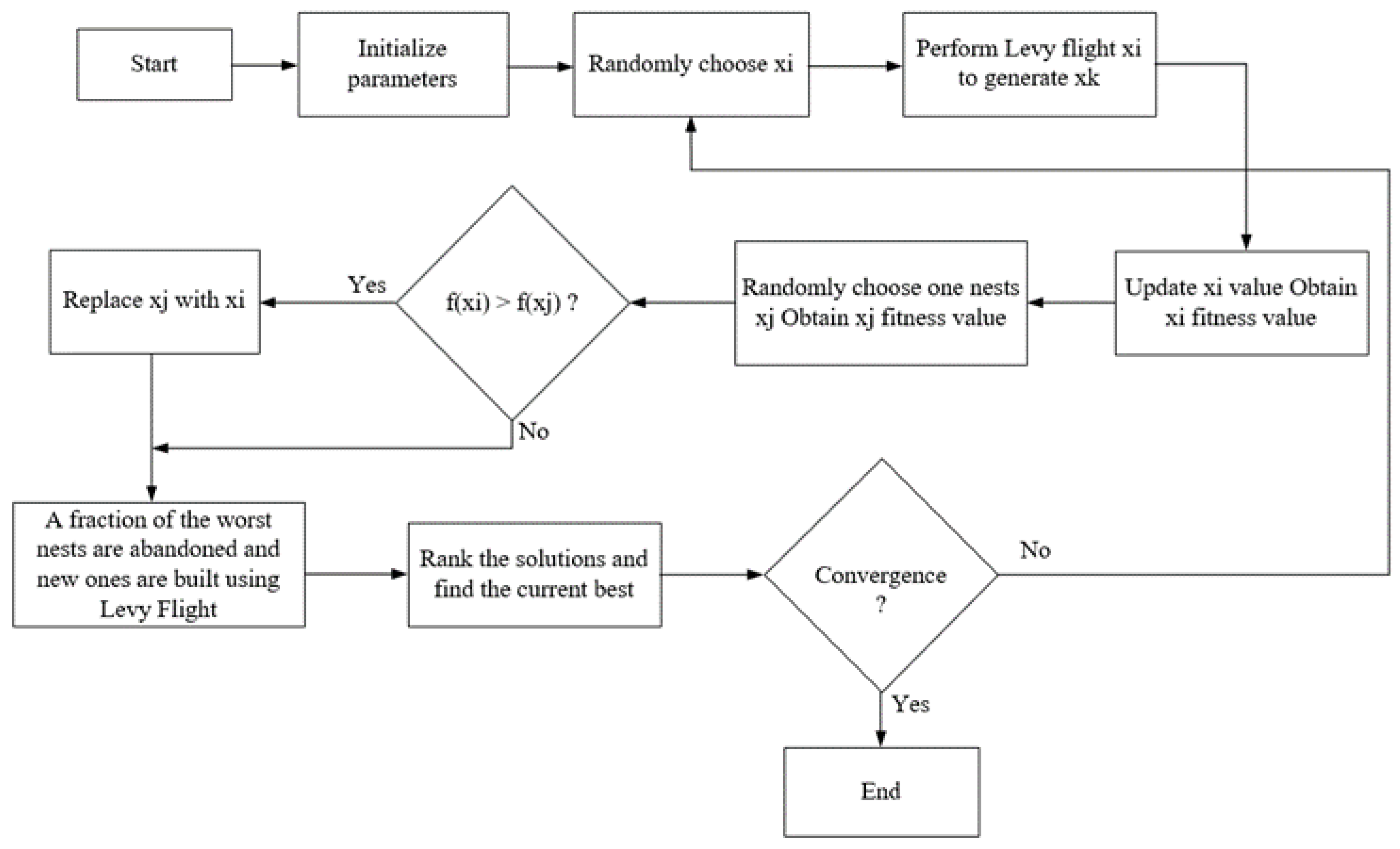
2.3. Cuckoo Search Algorithm (CSA)

The CSA is one of the new-generation smart methods developed by Xin-She Yang and Suash Deb in 2009. It is a population-based algorithm. CSA is a method developed by observing the brood parasitism-based behaviors of some cuckoos [50,51]. The CSA has three main rules:

∗

Cuckoos lay only one egg at a time in a randomly selected nest.

∗

Those who have deposited eggs in the nests are transferred to the next generation.

∗

The number of host nests is fixed and, with probability 𝑝𝑎 ϵ (0,1), eggs laid by cuckoos can be recognized by the host nest owner [50,51]. The flowchart diagram of the CSA used in maximum power point tracking is shown in Figure 8 [52].

Searching for a suitable host nest is very important for the continuation of the cuckoo’s generation. The search for a nest is like the search for food, which occurs randomly or semi-randomly. In general, when searching for food, living things follow directions or trajectories that can be modeled with a precise mathematical function. The Lévy flight model is one of the most widely used models [53]. CSA benefits from Lévy flight. CSA achieves local maximum points due to Lévy flight. Additionally, it shortens the time it takes to reach the global maximum power point [54]. Lévy flight is a random method in which stride sizes are expressed in terms of stride lengths with a precise probability distribution [53]. Each egg in the host nest represents the CSA solution. It is aimed at hiding the solutions with a lot of potential. The Lévy flight is expressed in Equation (7) to create a new solution during iteration [55].

$${\mathrm{X}}_{\mathrm{i}}{}^{\mathrm{t}+1}={\mathrm{X}}_{\mathrm{i}}{}^{\mathrm{t}}+\mathrm{a}\oplus \mathrm{L}\mathrm{e}\mathrm{v}\mathrm{y}\left(\mathsf{\lambda }\right)$$

(7)

The random stride length is derived from a Lévy distribution. The mathematical expression of the Lévy distribution for random steps is given in Equation (8) [52].

$$\mathrm{L}\mathrm{e}\mathrm{v}\mathrm{y}\left(\mathsf{\lambda }\right)\approx {\mathrm{t}}^{-\mathsf{\lambda }},\begin{array}{cc}& 1<\mathsf{\lambda }\le 3\end{array}$$

(8)

α > 0 is the step size related to the size of the problem of interest and t is the number of iterations [56]. While performing MPPT with CSA, the duty cycle is selected as the control variable. The step size α is described as the difference between the best-existing sample and the other samples. β is expressed as the power-law index. u and v represent probabilistic design parameters with standard deviations, κ is the step coefficient, and Γ is the gamma function. The following equations are expressions describing the work of the CSA for MPPT [15].

$${\mathrm{V}}_{\mathrm{i}}{}^{\mathrm{t}+1}={\mathrm{V}}_{\mathrm{i}}{}^{\mathrm{t}}+\mathsf{\kappa }·\left(\frac{\mathrm{u}}{{\left|\mathrm{v}\right|}^{\raisebox{1ex}{$1$}\!\left/ \!\raisebox{-1ex}{$\mathsf{\beta }$}\right.}}\right)·\left({\mathrm{V}}_{\mathrm{b}\mathrm{e}\mathrm{s}\mathrm{t}}-{\mathrm{V}}_{\mathrm{i}}\right)$$

(9)

$$\mathrm{u}\approx \mathrm{N}\left(0,{\mathsf{\sigma }}_{\mathrm{u}}{}^2\right)\begin{array}{cc},& \mathrm{v}\approx \mathrm{N}\left(0,{\mathsf{\sigma }}_{\mathrm{v}}{}^2\right)\end{array}$$

(10)

$${\mathsf{\sigma }}_{\mathrm{u}}={\left(\frac{\mathsf{\Gamma }\left(1+\mathsf{\beta }\right)·\sin \left(\mathsf{\pi }·\raisebox{1ex}{$\mathsf{\beta }$}\!\left/ \!\raisebox{-1ex}{$2$}\right.\right)}{\mathsf{\Gamma }\left(\left(\frac{1+\mathsf{\beta }}{2}\right)\right)·\mathsf{\beta }·{\left(2\right)}^{\left(\frac{\mathsf{\beta }-1}{2}\right)}}\right)}^{\frac{1}{\mathsf{\beta }}}\begin{array}{cc},& {\mathsf{\sigma }}_{\mathrm{v}}=1\end{array}$$

(11)

At each iteration, Lévy flight is made by all particles until the GMPP is reached. The tracking process is terminated when a suitable result is reached [51].

One of the primary advantages of CSA use in MPPT is its capacity for efficient global optimization. With its stochastic nature, the global optimum of the MPPT problem can be searched efficiently by the CSA. The simplicity of the CSA algorithm makes the algorithm suitable for MPPT applications. CSA is less likely to be trapped in local optima due to its random nature, improving the robustness and reliability of the algorithm. Additionally, CSA’s parallel search capability makes it suitable for MPPT applications with multiple PV panels.

However, CSA has limitations when solving the MPPT problem. The first limitation is that CSA may converge slowly compared to other algorithms, such as the perturb and observe (P&O) algorithm or the incremental conductance algorithm. Another restriction of CSA is that it can be sensitive to its parameter values, such as the population size or the step size. Thirdly, CSA lacks strong theoretical guarantees for convergence or optimality. Finally, CSA may struggle to find the optimum of a complex and nonlinear objective function, which can be the case in some MPPT applications.

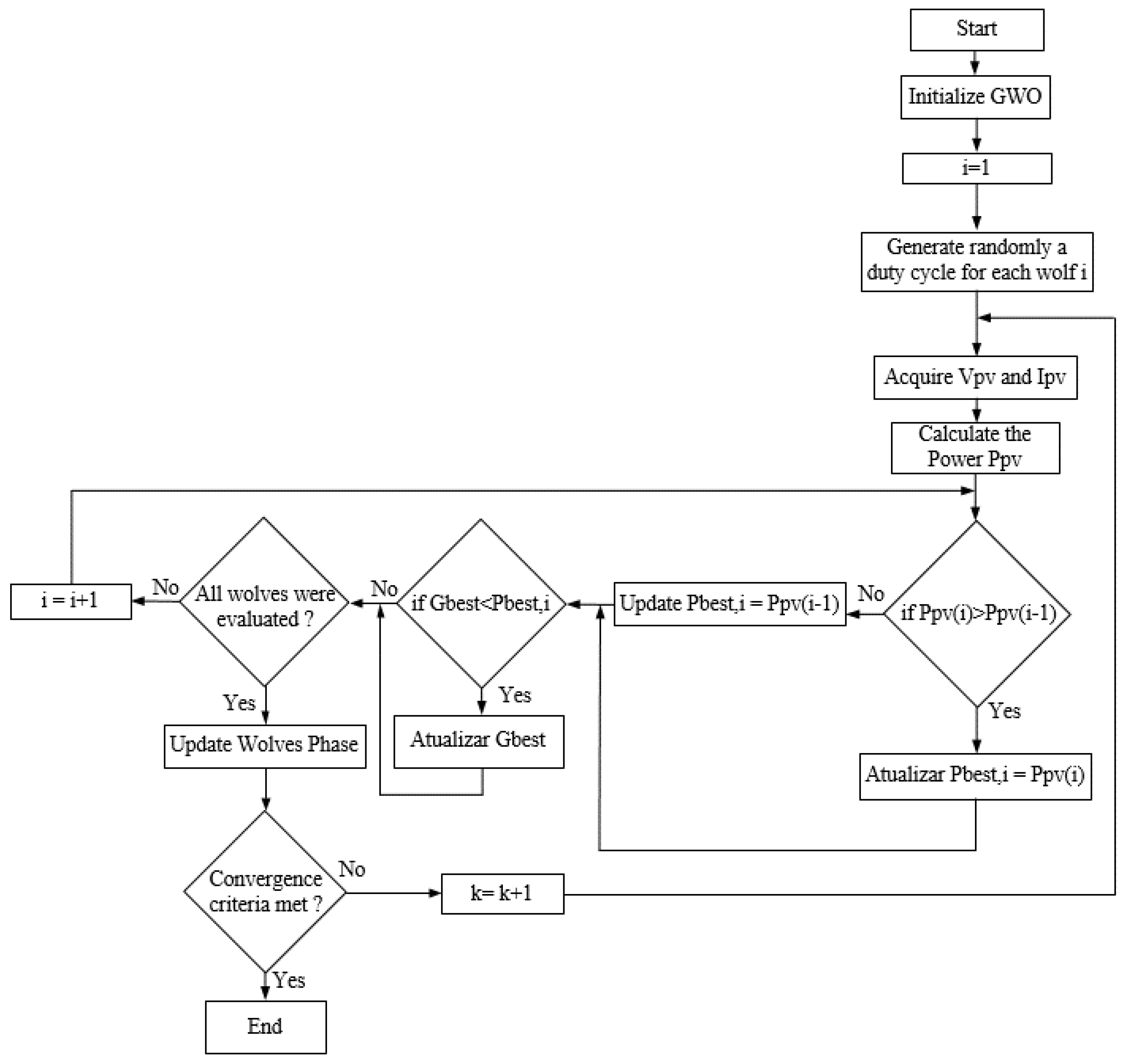
2.4. Grey Wolf Optimization Algorithm (GWO)

The GWO algorithm was developed by Seyedali Mirjalili in 2014. It is an intelligent optimization method based on swarm intelligence. While developing the method, Seyedali Mirjalili was inspired by the attack approach and social behavior of grey wolves during hunting. Grey wolves live in groups of about 5–12 members. In addition to the hunting efficiency of grey wolves, this method can also mimic social dominant hierarchy leadership. Grey wolves with this leadership hierarchy are grouped into alpha (α), beta (β), delta (δ), and omega (ω) [57]. Optimization includes three main stages; to follow the prey, to chase and approach, and then to surround the prey and attack. The hunting system of grey wolves is controlled by the alpha group, which is accepted as the leader or dominant wolf. It also has the authority to decide on the management, sleeping place and time of other wolves. Beta wolves follow the alpha and assist in group activities. This group is the strongest candidate for replacement if something happens to one of the alpha wolves. In third place in the hierarchy are the deltas. Delta wolves dominate only the omega group. This group consists of elders, sentries, scouts, hunters, and caregivers. Caregivers are responsible for caring for injured wolves during the hunting process. At the end of the hierarchy is the omega group. Omega wolves must always bow to the other three groups [57]. In this hunting system, the hunt represents GMPP. Therefore, it is used to overcome the multi-peak problems that occur in PV systems. This method is combined with direct duty cycle control. The aim here is to fix the duty cycle in GMPP and to minimize the steady-state oscillations [58]. The flowchart diagram of the GWO used in maximum power point tracking is shown in Figure 9.

Here, P_best,i indicates the best result in iterations, and G_best indicates the best result found by the wolves [59]. Equations (12) and (13) are used to show the hunting method of grey wolves.

$$\overrightarrow{\mathrm{D}}=\left|\overrightarrow{\mathrm{C}}·{\mathrm{X}}_{\mathrm{p}}(\mathrm{t})-\overrightarrow{\mathrm{X}}(\mathrm{t})\right|$$

(12)

$$\overrightarrow{\mathrm{X}}(\mathrm{t}+1)=\overrightarrow{{\mathrm{X}}_{\mathrm{p}}}(\mathrm{t})-\overrightarrow{\mathrm{A}}·\overrightarrow{\mathrm{D}}$$

(13)

Here, t shows the existing repetition; the coefficient vectors are D, A, and C. X_P represents the position vector of the prey and X represents the position vector of the grey wolf. The vectors A and C are calculated with Equation (14).

$$\overrightarrow{\mathrm{A}}=2\overrightarrow{\mathrm{a}·}\overrightarrow{{\mathrm{r}}_1}-\overrightarrow{\mathrm{a}}, \overrightarrow{\mathrm{C}}=2·\overrightarrow{{\mathrm{r}}_2}$$

(14)

Here, the value of α is linearly decreased from 2 to 0. The values of the r₁ and r₂ vectors are in the range [0, 1]. In a GWO-based MPPT study, D represents the grey wolf. Therefore, it can be restarted with Equations (15) and (16).

$${\mathrm{D}}_{\mathrm{i}}(\mathrm{k}+1)={\mathrm{D}}_{\mathrm{i}}(\mathrm{k})-\mathrm{A}·\mathrm{D}$$

(15)

$$\mathrm{P}\left({\mathrm{d}}_{\mathrm{i}}{}^{\mathrm{k}}\right)>\mathrm{P}\left({\mathrm{d}}_{\mathrm{i}}{}^{\mathrm{k}-1}\right)$$

(16)

In Equations (15) and (16), P denotes power, D refers to the duty cycle, i represents the number of grey wolves present, and k represents the number of iterations. One of the most important contributions of this method is that it eliminates steady-state oscillations [16]. In MPPT optimization use, the GWO algorithm is preferred because of its capability to achieve a better trade-off between exploration and exploitation compared to other algorithms. GWA makes the transition quickly to the global optimum and maintains it for a longer time. Moreover, by using a Pareto-based approach, multiple objective functions can be handled. Another strength of GWA is its ability to converge faster than some other optimization algorithms. The primary limitation of GWO is the difficulty in setting the appropriate parameter values, such as the population size or the scaling factor, requiring careful parameter tuning. In addition, GWA may be susceptible to premature convergence, which may limit the search space. Finally, the computational complexity of GWA can be relatively high for large-scale MPPT applications.

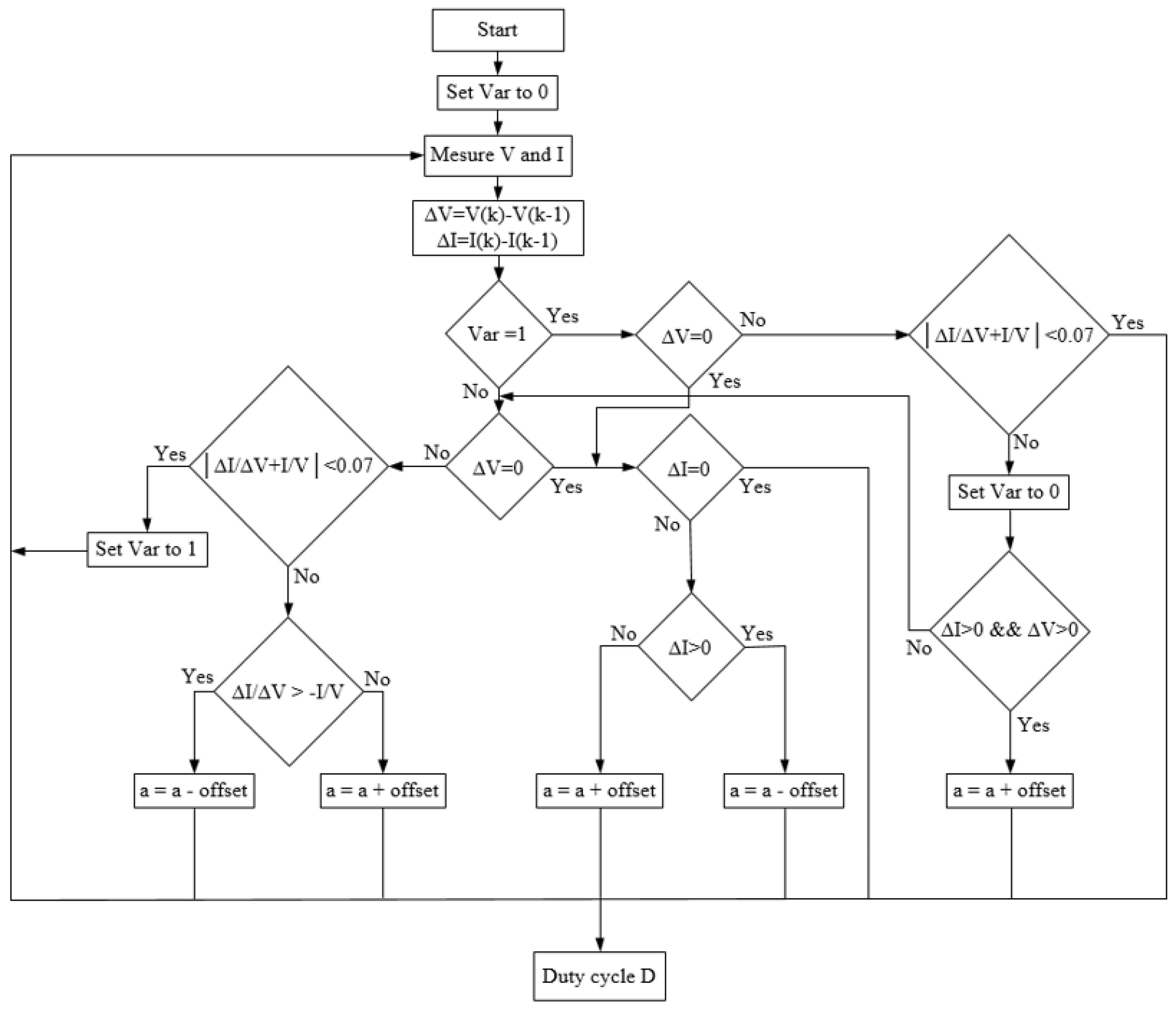
2.5. Modified Incremental Conductivity Algorithm (MIC)

A successful MPPT method provides a balance between tracking speed and steady state. In line with these conditions, the conventional incremental conductivity algorithm may not be able to properly track the MPPT in the case of a sudden change in irradiation. This can lead to low power efficiency [60]. For this reason, the idea has emerged of developing a conventional incremental conductivity algorithm. The flowchart diagram of the proposed MIC for maximum power point tracking is shown in Figure 10.

In the MIC method, as the sunlight begins to increase, the voltage and current values begin to increase. It is determined whether MPP is caught or not using both the increase in solar irradiation and the increase in the current and voltage. A permissive error is accepted to understand that the MPP has been caught. This error is expressed by Equation (17).

$$\left|\frac{\mathrm{d}\mathrm{I}}{\mathrm{d}\mathrm{V}}+\frac{\mathrm{I}}{\mathrm{V}}\right|<0.07$$

(17)

The proposed method provides an optimizing feature that checks if the MPP is caught and then sets the reactive power value to one [61]. When the above equality is not met and the value of the reactive power is one, the proposed method checks whether the current and voltage values increase. In this situation, the proposed method increases the D instead of reducing it, unlike the conventional IC. As a result, the MIC method is developed to overcome the wrong response given by the conventional IC when the irradiance is increased [62].

The MIC algorithm is utilized in MPPTs for its ability to track the maximum power point (MPP) accurately under rapidly changing environmental conditions. The MIC algorithm can quickly adapt to changes in the environment and adjust the operating point to the new MPP. Additionally, the MIC algorithm does not require any knowledge of the PV system’s parameters, making it easier to implement in practical applications.

Nevertheless, the MIC algorithm also has some limitations. One of the main limitations is its tendency to oscillate around the MPP under steady-state conditions, which can result in reduced efficiency and power output. The MIC algorithm may also fail to converge to the global MPP under certain conditions, such as partial shading or multiple local maxima. Additionally, the MIC algorithm requires the PV system to operate at a higher voltage than the MPP voltage to ensure accurate tracking, which can lead to power losses.

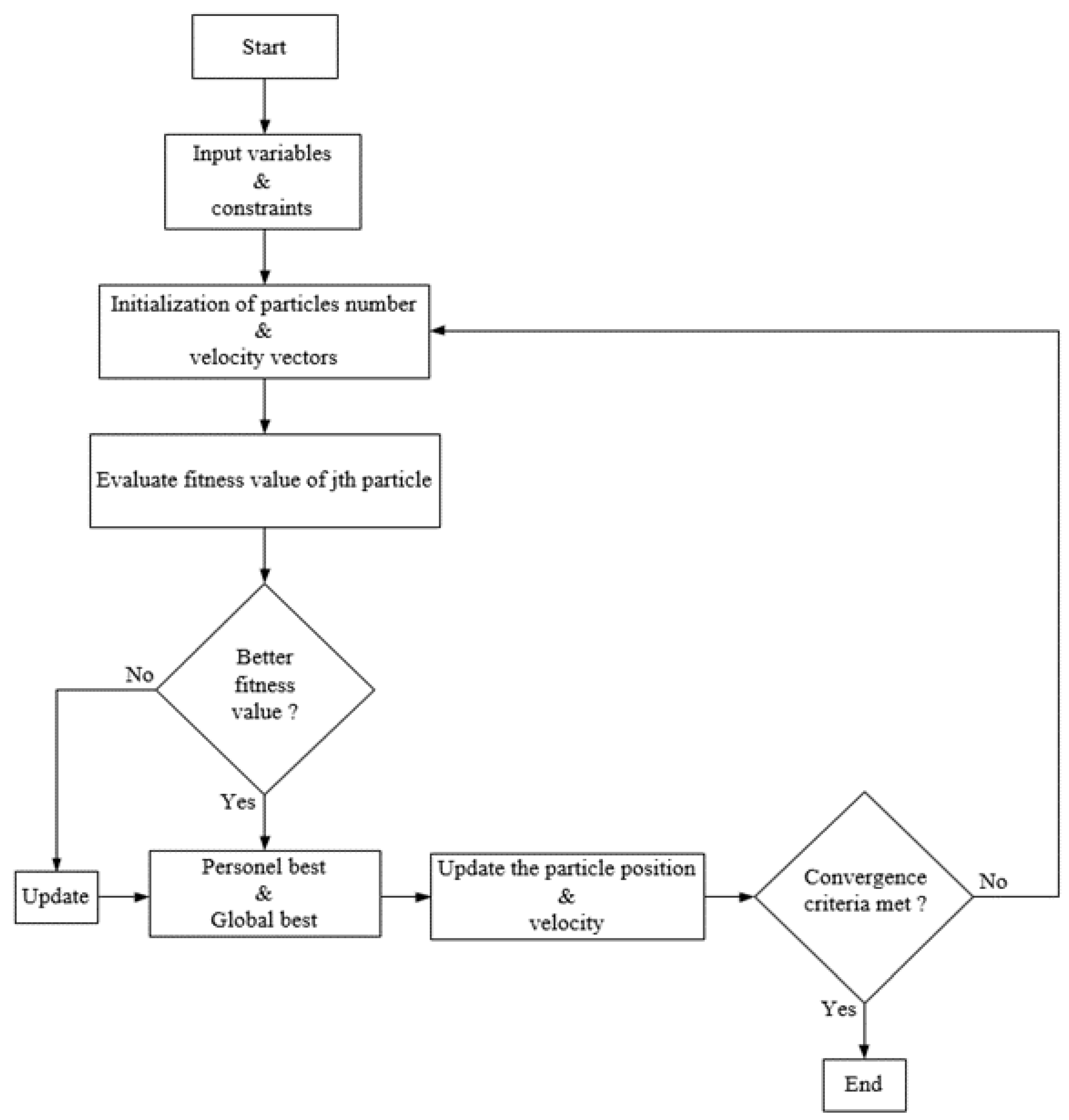
2.6. Particle Swarm Optimization Algorithm (PSO)

The PSO algorithm, which is among the most popular bio-inspired algorithms, is a probabilistic technique developed by Eberhart and Kennedy in 1995. The basis for this optimization was laid by observing the social behavior of creatures that move in flocks, such as birds and fish [63]. PSO is an unconventional, smart, easy-to-understand, and effective approach [64]. PSO handles the solution of the optimization problem in an n-dimensional field in the following way: Everyone arranges their flight direction according to their flight direction, as in bird flocks and the flight direction of the whole flock. In other words, in this method, individuals benefit from their past experiences of themselves and of the whole swarm. Everyone in this n-dimensional field is called a particle. Particles are used to provide searches for the optimal point. Therefore, each particle helps in the analysis of the optimization [65]. The flowchart diagram of the PSO algorithm is given in Figure 11.

When the flowchart is examined, after the PSO starts working, each particle updates its position and velocity. The particles then reach the optimum point by repeating each other. At all iteration stages, all particles are refreshed with the two best values. The first is the personal best value of particles available in the population. It is expressed as P_best,i. The second is the global best value obtained through particles in the population. It is expressed as G_best [67]. During the iteration process, the particles in the population have a fitness value that is decided by the fitness function. Additionally, they have a velocity that is used to decide the particle’s flight range and direction. After the P_best,i and G_best are found, the position and velocity information of each particle is updated with the relevant mathematical equations [68]. One of the most successful properties of the PSO algorithm, when used in MPPT, is its ability to converge to the global maximum power point (MPP) quickly and accurately, even under partial shading and multiple local maxima conditions. Additionally, the PSO algorithm can function without exact knowledge of the PV system’s parameters, making it easier to implement in practical applications. One of the downsides of this algorithm is its tendency to get stuck in local optima, especially in high-dimensional search spaces. This can lead to reduced efficiency and power output. Moreover, the PSO algorithm can suffer from premature convergence, which occurs when the algorithm stops exploring the search space too early and fails to find the global MPP. Furthermore, the PSO algorithm requires many iterations to converge to the MPP, which can increase the computational time and energy consumption of the PV system.

$${\mathrm{X}}_{\mathrm{i}}(\mathrm{k}+1)={\mathrm{X}}_{\mathrm{i}}(\mathrm{k})+{\mathrm{V}}_{\mathrm{i}}(\mathrm{k}+1)$$

(18)

$${\mathrm{V}}_{\mathrm{i}}(\mathrm{k}+1)=\mathrm{w}·{\mathrm{V}}_{\mathrm{i}}(\mathrm{k})+{\mathrm{c}}_1·{\mathrm{r}}_1\left[{\mathrm{P}}_{\mathrm{b}\mathrm{e}\mathrm{s}\mathrm{t}}-{\mathrm{X}}_{\mathrm{i}}(\mathrm{k})\right]+{\mathrm{c}}_2·{\mathrm{r}}_2\left[{\mathrm{G}}_{\mathrm{b}\mathrm{e}\mathrm{s}\mathrm{t}}-{\mathrm{X}}_{\mathrm{i}}(\mathrm{k})\right]$$

(19)

In Equations (18) and (19); i refers to the number of particles in the swarm, k refers to the number of iterations, w refers to the inertia weight, r₁ and r₂ refer to variables in the randomly distributed range [0, 1], and c₁ and c₂ refer to the acceleration coefficients. P_best,i, and X_i(k) express the best location of the particle, and G_best refers to the best location of particles in the swarm. X_i(k + 1) expresses the location of the particle. V_i(k + 1) refers to the velocity of the particle.

The function of variables c₁, c₂, and w is to control the convergence of the global search result to the best solution [69]. Another task of the inertia weight w is to balance between local and global search steps. c₁ affects the cognitive element of the particles in the population, and c₂ affects the social element. The search for optimum convergence is carried out through these two elements. For this reason, it is very important to properly control the acceleration coefficients. c₁ performs the operation of directing the particles in the population towards their personal best solution. c₂ directs the particles towards the best global value found so far between the repeat steps. The position of all particles is evaluated with a fitness function. When the maximum number of iterations is reached, the PSO is stopped [70].

3. Findings and Discussion

3.1. Result Obtained from the Designed System

In the system created, six PV panels were connected in series to each other. The uniform and complex shading conditions were applied to the system, respectively. The power values of the PV panels under different shading conditions are shown in

Table 2. Uniform and complex partial shading conditions.

Panel	1. UIC (W/m2)	2. CPSC (W/m2)	3. CPSC (W/m2)	4. CPSC (W/m2)	5. CPSC (W/m2)
Panel 1	1000	1200	350	150	1000
Panel 2	1000	1000	950	450	800
Panel 3	1000	800	900	550	950
Panel 4	1000	600	700	750	750
Panel 5	1000	400	500	850	900
Panel 6	1000	200	300	1100	650

. As a result of these values, current–voltage (I-V) and power–voltage (P-V) characteristic curves were obtained.

The current–voltage (I-V) and power–voltage (P-V) characteristic curves under different shading conditions are given in Figure 12. The first uniform irradiation condition (UIC) graph is given in Figure 12a. In the power–voltage graph in Figure 12a, only one peak occurs as each panel receives equal irradiance values. The maximum power value of this point is 1494 W. The second complex partial shading condition (CPSC) graph is given in Figure 12b. In Figure 12b, the global maximum power point is 664 W. The third CPSC graph is given in Figure 12c. In Figure 12c, the global maximum power point is 554 W. The fourth CPSC graph is given in Figure 12d. In Figure 12d, the global maximum power point is 634 W. The fifth CPSC graph is given in Figure 12e. In Figure 12e, the global maximum power point is 1080 W.

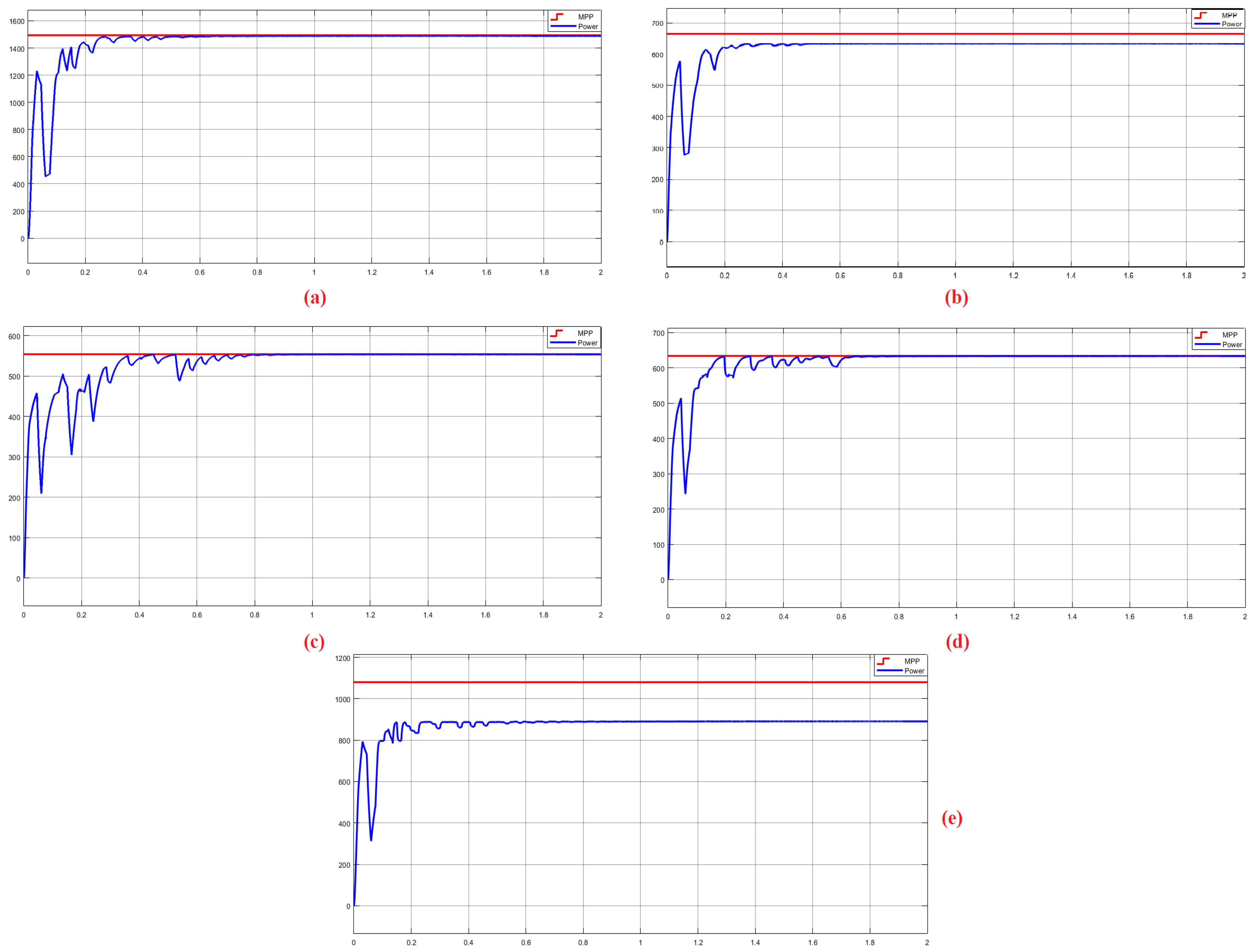
3.2. Modeling the Designed System with Cuckoo Search Optimization Algorithm

The power–time graph of CSA under different shading conditions is given in Figure 13. The first UIC graph is given in Figure 13a. When the first UIC graph is examined, it is seen that 1489 W power was obtained. It reached the global maximum power point in 0.48 s and maintained its stability. There was no oscillation. The efficiency of the system was calculated as 99.66%. The second CPSC power–time graph of CSA is given in Figure 13b. In Figure 13b, 633.5 W power was obtained. It could not reach the global maximum power point. It was caught at the local maximum power point. There was no oscillation. The efficiency of the system was calculated as 95.40%. The third CPSC power-time graph of CSA is given in Figure 13c. In Figure 13c, 553.5 W power was obtained. It reached the global maximum power point in 0.88 s and maintained its stability. There was no oscillation. The efficiency of the system was calculated as 99.90%. The fourth CPSC power–time graph of CSA is given in Figure 13d. In Figure 13d, 631 W power was obtained. It reached the global maximum power point in 0.65 s and maintained its stability. There was no oscillation. The efficiency of the system was calculated as 99.52%. The fifth CPSC power-time graph of CSA is given in Figure 13e. In Figure 13e, 890 W power was obtained. It could not reach the global maximum power point. It was caught at the local maximum power point. There was no oscillation. The efficiency of the system was calculated as 82.40%.

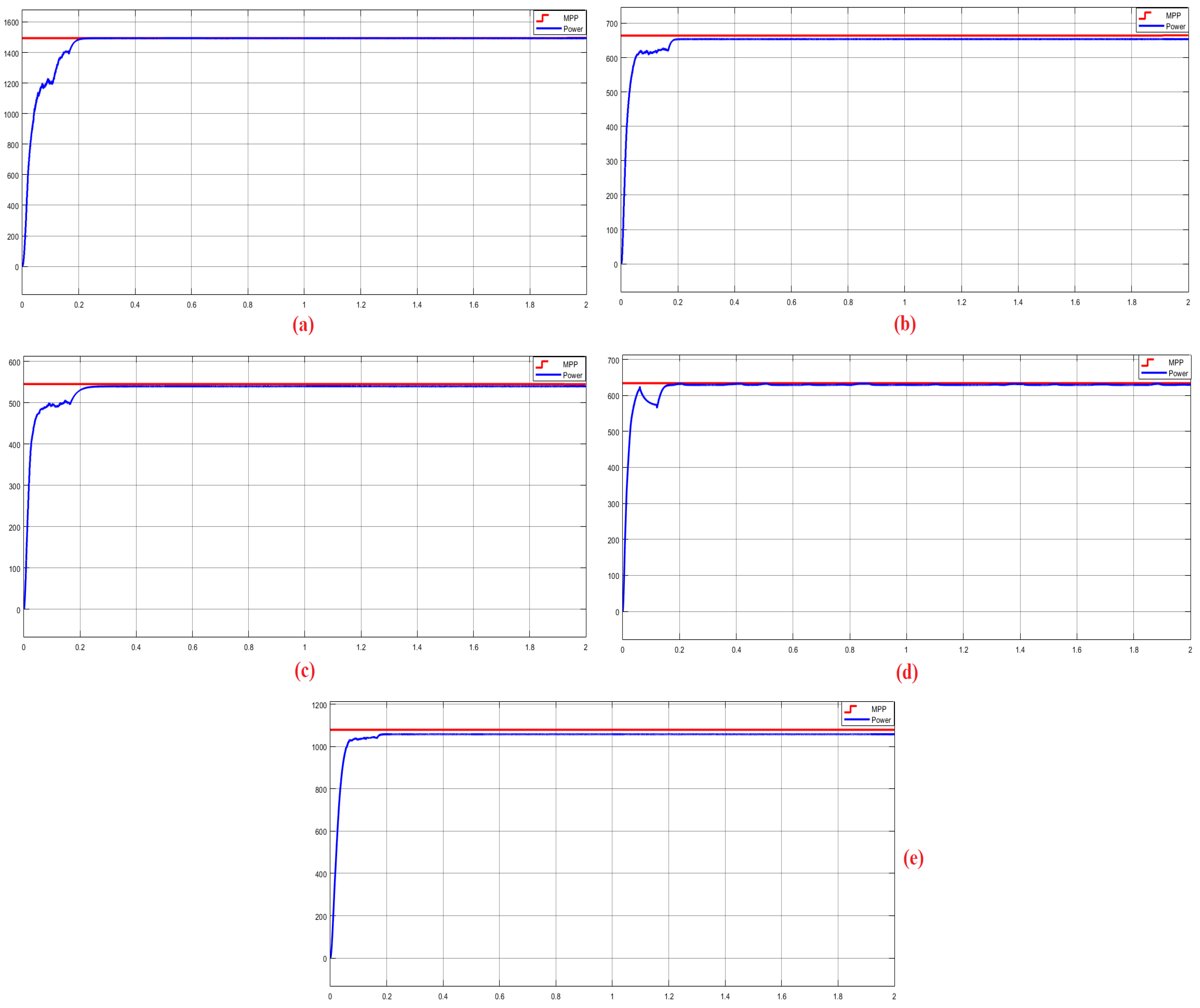
3.3. Modeling the Designed System with Grey Wolf Optimization Algorithm

The power–time graph of GWO under different shading conditions is given in Figure 13. The first UIC graph is given in Figure 14a. When the first UIC graph is examined, it is seen that 1493.9 W power was obtained. It reached the global maximum power point in 0.25 s and maintained its stability. There was no oscillation. The efficiency of the system was calculated as 99.99%. The second CPSC power-time graph of GWO is given in Figure 14b. In Figure 14b, 653.5 W power was obtained. It reached the global maximum power point in 0.2 s and maintained its stability. There was no oscillation. The efficiency of the system was calculated as 98.41%. The third CPSC power-time graph of GWO is given in Figure 14c. In Figure 14c, 548.5 W power was obtained. It reached the global maximum power point in 0.29 s and maintained its stability. There was no oscillation. The efficiency of the system was calculated as 99.00%. The fourth CPSC power-time graph of GWO is given in Figure 14d. In Figure 14d, 630 W power was obtained. It reached the global maximum power point in 0.21 s and maintained its stability. There was no oscillation. The efficiency of the system was calculated as 99.36%. The fifth CPSC power-time graph of GWO is given in Figure 14e. In Figure 14e, 1061 W power was obtained. It reached the global maximum power point in 0.19 s and maintained its stability. There was no oscillation. The efficiency of the system was calculated as 98.24%.

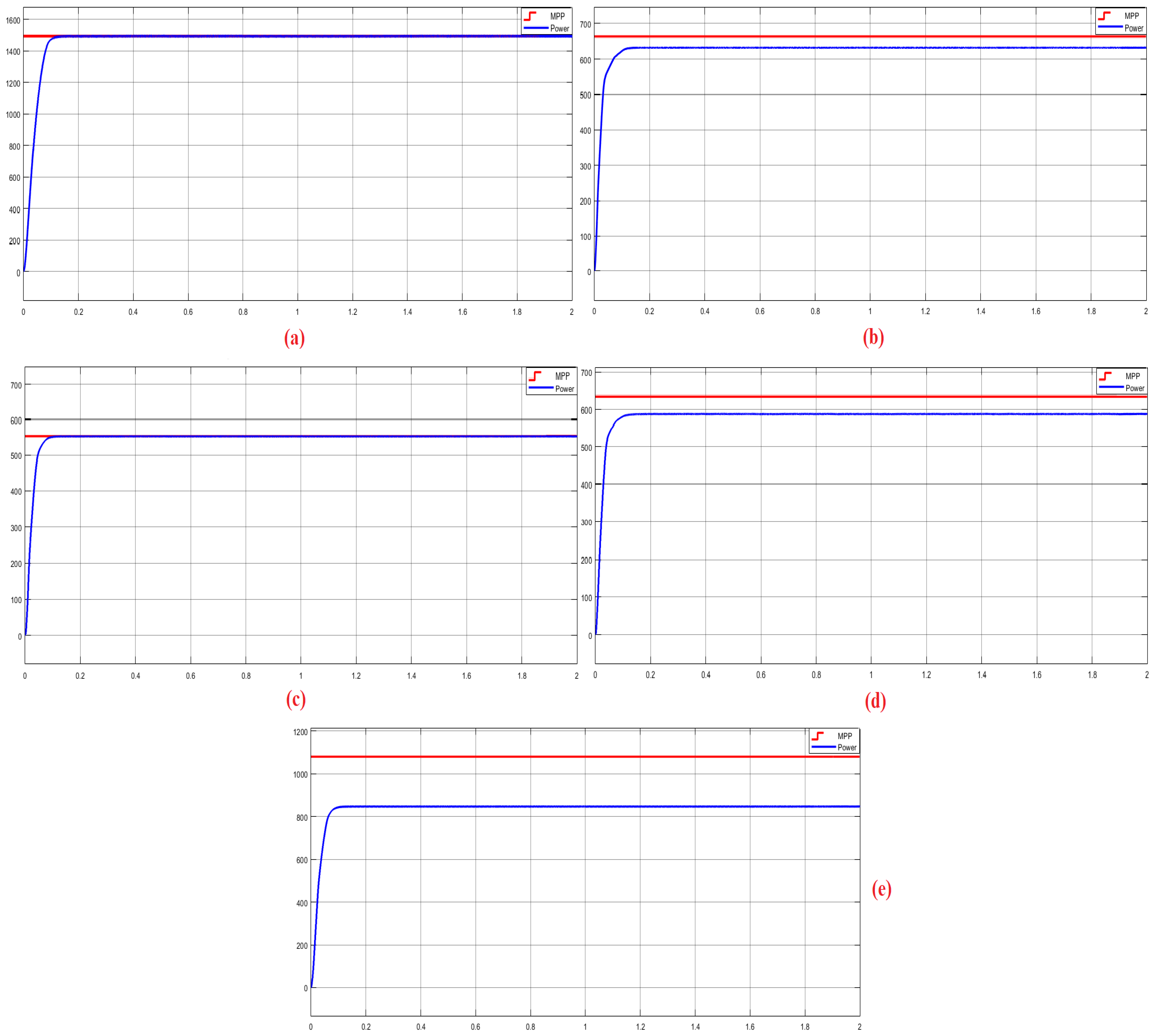
3.4. Modeling the Designed System with Modified Incremental Conductivity Algorithm

The power–time graph of MIC under different shading conditions is given in Figure 15. The first UIC graph is given in Figure 15a. When the first UIC graph is examined, it is seen that 1493.5 W power was obtained. It reached the global maximum power point in 0.16 s and maintained its stability. There was no oscillation. The efficiency of the system was calculated as 99.96%.

The second CPSC power–time graph of MIC is given in Figure 15b. In Figure 15b, 633.5 W power was obtained. It could not reach the global maximum power point. It was caught at the local maximum power point. There was no oscillation. The efficiency of the system was calculated as 95.40%. The third CPSC power-time graph of MIC is given in Figure 15c. In Figure 15c, 553.5 W power was obtained. It reached the global maximum power point in 0.14 s and maintained its stability. There was no oscillation. The efficiency of the system was calculated as 99.90%. The fourth CPSC power-time graph of MIC is given in Figure 15d. In Figure 15d, 588.5 W power was obtained. It could not reach the global maximum power point. It was caught at the local maximum power point. There was no oscillation. The efficiency of the system was calculated as 92.82%. The fifth CPSC power-time graph of MIC is given in Figure 15e. In Figure 15e, 847 W power was obtained. It could not reach the global maximum power point. It was caught at the local maximum power point. There was no oscillation. The efficiency of the system was calculated as 78.42%.

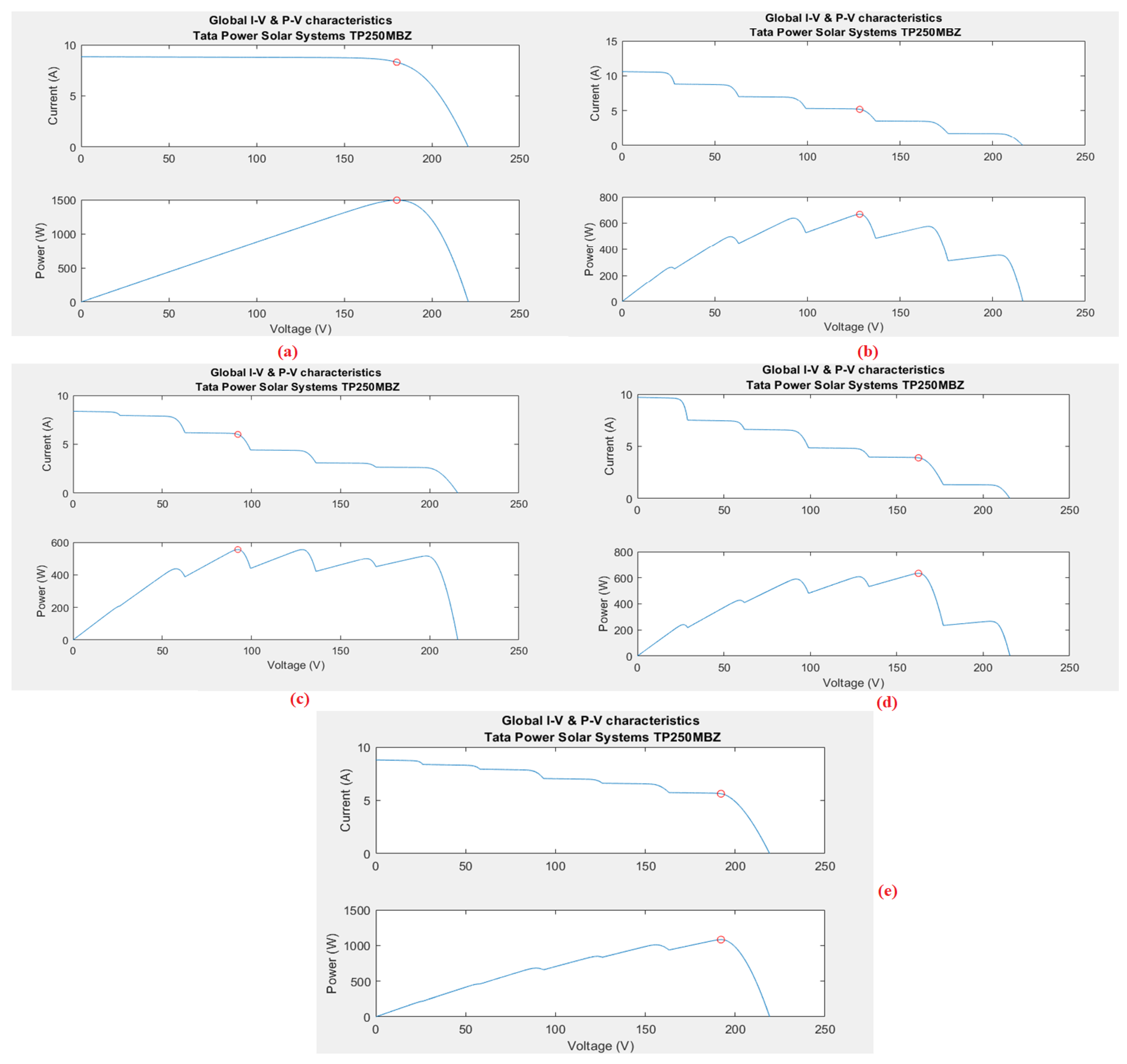
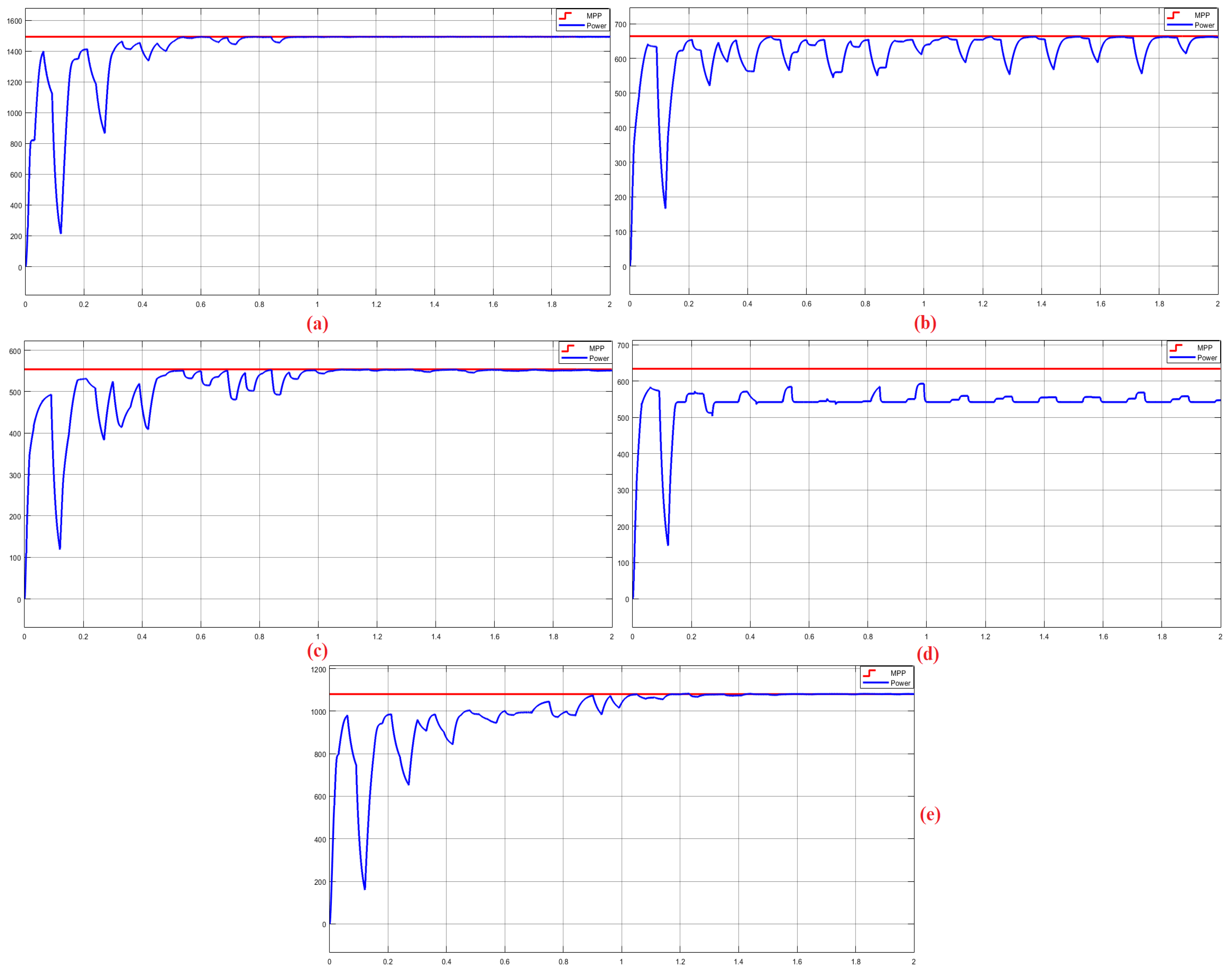
3.5. Modeling the Designed System with Particle Swarm Optimization Algorithm

The power-time graph of PSO under different shading conditions is given in Figure 16. The first UIC graph is given in Figure 16a. When the first UIC graph is examined, it is seen that 1493.5 W power was obtained. It reached the global maximum power point in 0.92 s and maintained its stability. There was no oscillation. The efficiency of the system was calculated as 99.96%.

The second CPSC power–time graph of PSO is given in Figure 16b. In Figure 16b, 662 W power was obtained. It reached the global maximum power point in 1.35 s and maintained its stability. There was an oscillation of 111.5 W and it was calculated as 16.84%. The efficiency of the system was calculated as 99.69%. The third CPSC power-time graph of PSO is given in Figure 16c. In Figure 16c, 552.5 W power was obtained. It reached the global maximum power point in 1.08 s and maintained its stability. There was an oscillation of 2.5 W and it was calculated as 0.45%. The efficiency of the system was calculated as 99.72%. The fourth CPSC power-time graph of PSO is given in Figure 16d. In Figure 16d, 542 W power was obtained. It could not reach the global maximum power point. It was caught at the local maximum power point. There was an oscillation of 4.98 W in this graph and its oscillation was calculated as 0.92%. The efficiency of the system was calculated as 85.48%. The fifth CPSC power–time graph of PSO is given in Figure 16e. In Figure 16e, 1077.5 W power was obtained. It reached the global maximum power point in 1.18 s and maintained its stability. There was no oscillation. The efficiency of the system was calculated as 99.76%.

The values in the graphs obtained for each algorithm are recorded in

Table 3. Comparison of CSA, GWO, MIC, and PSO algorithms.

Shading	Algorithm	Power (W)	Efficiency (η)	Convergence Speed (s)	Oscillation (%)
1. UIC	CSA	1489 W	99.66%	0.48	0
	GWO	1493.9 W	99.99%	0.25	0
	MIC	1493.5 W	99.96%	0.16	0
	PSO	1493.5 W	99.96%	0.92	0
2. CPSC	CSA	633.5 W	95.40%	0.49	0
	GWO	653.5 W	98.41%	0.20	0
	MIC	633.5 W	95.40%	0.15	0
	PSO	662 W	99.69%	1.35	16.84
3. CPSC	CSA	553.5 W	99.90%	0.88	0
	GWO	548.5 W	99.00%	0.29	0
	MIC	553.5 W	99.90%	0.14	0
	PSO	552.5 W	99.72%	1.08	0.45
4. CPSC	CSA	631 W	99.52%	0.65	0
	GWO	630 W	99.36%	0.21	0
	MIC	588.5 W	92.82%	0.14	0
	PSO	542 W	85.48%	1.95	0.92
5. CPSC	CSA	890 W	82.40%	0.79	0
	GWO	1061 W	98.24%	0.19	0
	MIC	847 W	78.42%	0.15	0
	PSO	1077.5 W	99.76%	1.18	0

. In Table 3, the performance of the CSA, GWO, MIC, and PSO algorithms is compared to each other in terms of power, efficiency, convergence speed, and oscillation criteria. In Table 3, it is seen that the first and third cases are the cases where all the algorithms successfully track the global maximum power point at the same time. However, the same is not true for the other complex partial shading conditions. When the table is carefully examined, it is seen that only GWO achieved the global maximum power point with high convergence speed and efficiency for all complex partial shading situations. It is seen that the GWO did not oscillate while following the maximum power point. The average convergence speed of the GWO to the maximum power point was obtained as 0.22 s. The average efficiency of GWO was obtained as 99%. All these evaluations show that GWO is a very fast, efficient, and stable MPPT method under complex partial shading conditions.

In Table 3, the productivity and convergence speed and oscillation parameters are used to evaluate the optimization algorithms. The efficiency parameter measures the ratio of the power output of the PV panel to the maximum power that could be obtained at a given irradiance and temperature. A high tracking efficiency indicates that the algorithm can effectively track the maximum power point under varying environmental conditions. Another parameter is the convergence speed. This parameter shows how quickly the algorithm responds to changes in the maximum power point. A fast-tracking speed is important for ensuring that the algorithm can quickly and accurately track the maximum power point as environmental conditions change. The oscillation parameter in maximum power point tracking (MPPT) refers to the tendency of the MPPT algorithm to oscillate around the true maximum power point, leading to fluctuations in the output power of the photovoltaic system.

4. Conclusions

Intelligent methods are frequently used while tracking the global maximum power point under partial shading conditions in PV systems. These methods can easily capture and track the global maximum power point under partial shading conditions with two or three peaks. However, under multiple peaks of more than two or three, they may fail to catch and track the global maximum power point. In the proposed method, when there is a change in the radiation intensity, a capacitor is connected to the PV array as a load, and the P–V curve of the array is obtained by the controller according to the current environmental conditions. An adaptive circuit structure is proposed for capacitor charging. Thus, the efficiency of the system is increased, and the circuit area and cost are reduced. While the power amount can be increased by approximately 150% compared to the conventional circuit, the power losses to be obtained were confirmed by the experimental results. The experimental setup prepared for this purpose was controlled with an FPGA control card. On an array of six panels, both full irradiation and different partial shadow states were created. The electrical characteristics of the PV system corresponding to the current situation and the power and voltage values of the GMPP were determined by the load device.

This study was carried out to investigate which of the smart methods used was more efficient when performing global maximum power point tracking of PV energy systems under complex partial shading conditions. For this reason, a system was designed in MATLAB-Simulink software. The intelligent algorithms, CSA, GWO, MIC, and PSO, were used as MPPT methods in the designed system. As a result of the simulations, these algorithms were compared in Table 2 in terms of power, convergence speed, efficiency, and oscillation criteria. These algorithms were run under five different uniform and complex partial shading conditions with six PV panels connected in series and a DC–DC boost converter. Since each PV panel was exposed to different irradiance values, six different peaks occurred. Only one of these peaks was the global maximum power point and the others were local maximum power points. Therefore, under this six-peak complex condition, it was even more difficult for the algorithms to catch and track the global maximum power point.

According to the simulation results in this study, it was seen that the first and third cases were the cases where all the algorithms successfully tracked the global maximum power point at the same time. However, the same was not true for the other complex partial shading conditions. Despite this complexity and difficulty, GWO was successful in the simulations. Compared to the other algorithms, it was observed that GWO successfully performed global maximum power point tracking with high convergence ability and tracking speed in all five conditions. It was observed that GWO did not oscillate while tracking the global maximum power point. The fact that GWO did not oscillate reduced power losses and, therefore, increased efficiency. The average convergence speed of GWO to the global maximum power point was obtained as 0.22 s. The average efficiency of GWO was obtained as 99%. All these evaluations show that GWO is a very fast, highly accurate, efficient, and stable MPPT method under complex partial shading conditions. In future studies, it is anticipated that efficiency analyses will be undertaken using the designed system and GWO, running them with real-time data.

References

1. Sanseverino, E.R.; Ngoc, T.N.; Cardinale, M.; Li Vigni, V.; Musso, D.; Romano, P.; Viola, F. Dynamic programming and Munkres algorithm for optimal photovoltaic arrays reconfiguration. Sol. Energy 2015, 122, 347–358. [Google Scholar] [CrossRef]
2. Zhang, H.; Lu, Z.; Hu, W.; Wang, Y.; Dong, L.; Zhang, J. Coordinated optimal operation of hydro-wind-solar integrated systems. Appl. Energy 2019, 242, 883–896. [Google Scholar] [CrossRef]
3. Kabalci, E. Maximum power point tracking (MPPT) algorithms for photovoltaic systems. In Energy Harvesting and Energy Efficiency, Technology, Methods, and Applications, 1st ed.; Lecture Notes in Energy; Bizon, N., Mahdavi Tabatabaei, N., Blaabjerg, F., Kurt, E., Eds.; Springer: Cham, Switzerland, 2017; Volume 37, pp. 205–234. [Google Scholar]
4. Podder, A.K.; Roy, N.K.; Pota, H.R. MPPT methods for solar PV systems: A critical review based on tracking nature. IET Renew. Power Gener. 2019, 13, 1615–1632. [Google Scholar] [CrossRef]
5. Dali, A.; Abdelmalek, S.; Bakdi, A.; Bettayeb, M. A novel effective nonlinear state observer based robust nonlinear sliding mode controller for a 6 kW Proton Exchange Membrane Fuel Cell voltage regulation. Sustain. Energy Technol. Assess. 2021, 44, 100996. [Google Scholar] [CrossRef]
6. Ravyts, S.; Vecchia, M.D.; Van den Broeck, G.; Yordanov, G.H.; Gonçalves, J.E.; Moschner, J.D.; Saelens, D.; Driesen, J. Embedded BIPV module-level DC/DC converters: Classification of optimal ratings. Renew. Energy 2020, 146, 880–889. [Google Scholar] [CrossRef]
7. Anwer, A.M.O.; Omar, F.A.; Bakir, H.; Kulaksiz, A.A. Sensorless control of a PMSM drive using EKF for wide speed range supplied by MPPT based solar PV system. Elektron. Ir Elektrotechnika 2020, 26, 32–39. [Google Scholar] [CrossRef] [Green Version]
8. Karami, N.; Moubayed, N.; Outbib, R. General review and classification of different MPPT techniques. Renew. Sustain. Energy Rev. 2017, 68, 1–18. [Google Scholar] [CrossRef]
9. Guiza, D.; Ounnas, D.; Soufi, Y.; Bouden, A.; Maamri, M. Implementation of Modified Perturb and Observe Based MPPT Algorithm for Photovoltaic System. In Proceedings of the International Conference on Sustainable Renewable Energy Systems and Applications (ICSRESA), Tebessa, Algeria, 4–5 December 2019. [Google Scholar]
10. Ping, W.; Hui, D.; Changyu, D.; Shengbiao, Q. An Improved MPPT Algorithm Based on Traditional Incremental Conductance Method. In Proceedings of the 4th International Conference on Power Electronics Systems and Applications, Hong Kong, China, 8–10 June 2011. [Google Scholar]
11. Schoeman, J.J.; van Wyk, J.D. A Simplified Maximal Power Controller for Terrestrial Photovoltaic Panel Arrays. In Proceedings of the IEEE Power Electronics Specialists Conference, Cambridge, MA, USA, 14–17 June 1982; pp. 361–367. [Google Scholar]
12. Ankaiah, B.; Nageswararao, J. Enhancement of solar photovoltaic cell by using short-circuit current MPPT method. Int. J. Eng. Sci. Invent. 2013, 2, 45–50. [Google Scholar]
13. Gosumbonggot, J.; Fujita, G. Partial shading detection and global maximum power point tracking algorithm for photovoltaic with the variation of irradiation and temperature. Energies 2019, 12, 202. [Google Scholar] [CrossRef] [Green Version]
14. Avila, E.; Pozo, N.; Pozo, M.; Salazar, G.; Dominguez, X. Improved Particle Swarm Optimization Based MPPT for PV Systems Under Partial Shading Conditions. In Proceedings of the IEEE Southern Power Electronics Conference (SPEC), Puerto Varas, Chile, 4–7 December 2017. [Google Scholar]
15. Ahmed, J.; Salam, Z. A maximum power point tracking (MPPT) for PV system using cuckoo search with partial shading capability. Appl. Energy 2014, 119, 118–130. [Google Scholar] [CrossRef]
16. Mohapatra, A.; Nayak, B.; Das, P.; Mohanty, K.B. A review on MPPT techniques of PV system under partial shading condition. Renew. Sustain. Energy Rev. 2017, 80, 854–867. [Google Scholar] [CrossRef]
17. Sagonda, A.F.; Folly, K.A. Maximum Power Point Tracking in Solar PV Under Partial Shading Conditions Using Stochastic Optimization Techniques. In Proceedings of the IEEE Congress on Evolutionary Computation (CEC), Wellington, New Zealand, 10–13 June 2019; pp. 1967–1974. [Google Scholar]
18. Sawant, P.T.; Lbhattar, P.C.; Bhattar, C.L. Enhancement of PV System Based on Artificial Bee Colony Algorithm Under Dynamic Conditions. In Proceedings of the IEEE International Conference on Recent Trends in Electronics, Information & Communication Technology (RTEICT), Bangalore, India, 20–21 May 2016; pp. 1251–1255. [Google Scholar]
19. Besheer, A.H.; Adly, M. Ant Colony System Based PI Maximum Power Point Tracking for Stand Alone Photovoltaic System. In Proceedings of the IEEE International Conference on Industrial Technology, Athens, Greece, 19–21 March 2012; pp. 693–698. [Google Scholar]
20. Kaced, K.; Larbes, C.; Ramzan, N.; Bounabi, M.; Dahmane, Z.E. Bat algorithm based maximum power point tracking for photovoltaic system under partial shading conditions. Sol. Energy 2017, 158, 490–503. [Google Scholar] [CrossRef] [Green Version]
21. Kumar, C.H.S.; Rao, R.S. A novel global MPP tracking of photovoltaic system based on whale optimization algorithm. Int. J. Renew. Energy Dev. 2016, 5, 225–232. [Google Scholar] [CrossRef]
22. Aygul, K.; Cikan, M.; Demirdelen, T.; Tumay, M. Butterfly optimization algorithm based maximum power point tracking of photovoltaic systems under partial shading condition. Energy Sources Part A Recovery Utulization Environ. Eff. 2019, 1–19. [Google Scholar] [CrossRef]
23. Mirza, A.F.; Mansoor, M.; Ling, Q.; Yin, B.; Javed, M.Y. A salp-swarm optimization based MPPT technique for harvesting maximum energy from PV systems under partial shading conditions. Energy Convers. Manag. 2020, 209, 112625. [Google Scholar] [CrossRef]
24. Vasantharaj, S.; Vinodhkumar, G.; Sasikumar, M. Development of A Fuzzy Logic Based Photovoltaic Maximum Power Point Tracking Control System Using Boost Converter. In Proceedings of the IET Chennai 3rd International on Sustainable Energy and Intelligent Systems (SEISCON 2012), Tiruchengode, India, 27–29 December 2012. [Google Scholar]
25. Kulaksiz, A.A.; Akkaya, R. A genetic algorithm optimized ANN-based MPPT algorithm for a stand-alone PV system with induction motor drive. Sol. Energy 2012, 86, 2366–2375. [Google Scholar] [CrossRef]
26. Rizzo, S.A.; Scelba, G. ANN based MPPT method for rapidly variable shading conditions. Appl. Energy 2015, 145, 124–132. [Google Scholar] [CrossRef]
27. Mansoor, M.; Mirza, A.F.; Ling, Q. Harris hawk optimization-based MPPT control for PV systems under partial shading conditions. J. Clean. Prod. 2020, 274, 122857. [Google Scholar] [CrossRef]
28. Motamarri, R.; Bhookya, N. JAYA algorithm based on lévy flight for global MPPT under partial shading in photovoltaic system. IEEE J. Emerg. Sel. Top. Power Electron. 2020, 9, 4979–4991. [Google Scholar] [CrossRef]
29. Mohammadinodoushan, M.; Abbassi, R.; Jerbi, H.; Waly Ahmed, F.; Abdalqadir, K.; Ahmed, H.; Rezvani, A. A new MPPT design using variable step size perturb and observe method for PV system under partially shaded conditions by modified shuffled frog leaping algorithm-SMC controller. Sustain. Energy Technol. Assess. 2021, 45, 101056. [Google Scholar] [CrossRef]
30. Tey, K.S.; Mekhilef, S. Modified incremental conductance algorithm for photovoltaic system under partial shading conditions and load variation. IEEE Trans. Ind. Electron. 2014, 61, 5384–5392. [Google Scholar]
31. Babu, T.S.; Rajasekar, N.; Sangeetha, K. Modified particle swarm optimization technique based maximum power point tracking for uniform and under partial shading condition. Appl. Soft Comput. 2015, 34, 613–624. [Google Scholar] [CrossRef]
32. Omar, F.A.; Kulaksiz, A.A. Experimental evaluation of a hybrid global maximum power tracking algorithm based on modified firefly and perturbation and observation algorithms. Neural Comput. Appl. 2021, 33, 17185–17208. [Google Scholar] [CrossRef]
33. Kulaksız, A.A.; Akkaya, R. Training data optimization for ANNs using genetic algorithms to enhance MPPT efficiency of a stand-alone PV system. Turk. J. Electr. Eng. Comput. Sci. 2012, 20, 241–254. [Google Scholar] [CrossRef]
34. Manickam, C.; Raman, G.R.; Raman, G.P.; Ganesan, S.I.; Nagamani, C. A hybrid algorithm for tracking of GMPPT based on P&O and PSO with reduced power oscillation in string inverters. IEEE Trans. Ind. Electron. 2016, 63, 6097–6106. [Google Scholar]
35. Zhang, W.; Zhou, G.; Ni, H.; Sun, Y. A modified hybrid maximum power point tracking method for photovoltaic arrays under partially shading condition. IEEE Access 2019, 7, 160091–160100. [Google Scholar] [CrossRef]
36. Rocha, M.V.; Sampaio, L.P.; Silva, S.A.O. Comparative analysis of MPPT algorithms based on bat algorithm for PV systems under partial shading condition. Sustain. Energy Technol. Assess. 2020, 40, 100761. [Google Scholar] [CrossRef]
37. Özdemir, A.; Pamuk, N. Investigation of maximum power point tracking in complex photovoltaic energy systems under partial shading conditions using metaheuristic algorithms. Eur. J. Sci. Technol. 2021, 31 (Suppl. S1), 157–164. [Google Scholar]
38. Sameeullah, M.; Swarup, A. MPPT schemes for PV system under normal and partial shading condition: A review. Int. J. Renew. Energy Dev. 2016, 5, 79–94. [Google Scholar] [CrossRef] [Green Version]
39. Celikel, R.; Yilmaz, M.; Gundogdu, A. A voltage scanning-based MPPT method for PV power systems under complex partial shading conditions. Renew. Energy 2022, 184, 361–373. [Google Scholar] [CrossRef]
40. Luque, A.; Hegedus, S. Handbook of Photovoltaic Science and Engineering, 2nd ed.; John Wiley & Sons, Ltd.: West Sussex, UK, 2011; pp. 841–895. [Google Scholar]
41. Suryavanshiu, R.G.; Suryavanshi, S.R.; Joshi, D.R.; Magadum, R.B. Maximum Power Point Tracking of SPV at Varying Atmospheric Condition Using Genetic Algorithm. In Proceedings of the International Conference on Energy Systems and Applications, Pune, India, 30 October–1 November 2015; pp. 415–419. [Google Scholar]
42. Bulárka, S.; Gontean, A. Dynamic PV Array Reconfiguration Under Suboptimal Conditions in Hybrid Solar Energy Harvesting Systems. In Proceedings of the IEEE 23rd International Symposium for Design and Technology in Electronic Packaging (SIITME), Constanta, Romania, 26–29 October 2017; pp. 419–422. [Google Scholar]
43. Saad, E.; Helmy, S.; Elkoteshy, Y.; AbouZayed, U. Implementation of a Modified MPPT Strategy for Solar-PV Arrays Connected to Harmonic-Polluted Grids Under Partial Shading Conditions. In Proceedings of the International Telecommunications Conference (ITC-Egypt), Alexandria, Egypt, 13–15 July 2021. [Google Scholar]
44. Kaffash, M.; Javidi, M.H.; Darudi, A. A Combinational Maximum Power Point Tracking Algorithm in Photovoltaic Systems Under Partial Shading Conditions. In Proceedings of the Iranian Conference on Renewable Energy & Distributed Generation (ICREDG), Mashhad, Iran, 2–3 April 2016; pp. 103–107. [Google Scholar]
45. Omar, F.A. Artificial Intelligence-Based Maximum Power Point Tracking Controller for PV Modules under Partial Shading Conditions. Ph.D. Thesis, Selçuk University, Konya, Turkey, 2020. [Google Scholar]
46. Aashoor, F. Maximum Power Point Tracking Techniques for Photovoltaic Water Pumping Systems. Ph.D. Thesis, University of Bath, Bath, UK, 2015. [Google Scholar]
47. Rashid, A.H. Power Electronics Handbook, 4th ed.; Butterworth-Heinemann: Oxford, UK, 2018; pp. 15–48. [Google Scholar]
48. Santos, J.L.; Antunes, F.; Chehab, A.; Cruz, C. A maximum power point tracker for FV systems using a high performance boost converter. Sol. Energy 2006, 80, 772–778. [Google Scholar] [CrossRef]
49. Esram, T.; Chapman, P.L. Comparison of photovoltaic array maximum power point tracking techniques. IEEE Trans. Energy Convers. 2007, 22, 439–449. [Google Scholar] [CrossRef] [Green Version]
50. Nugraha, D.A.; Lian, K.L.; Suwarno. A novel MPPT method based on cuckoo search algorithm and golden section search algorithm for partially shaded PV system. Can. J. Electr. Comput. Eng. 2019, 42, 173–182. [Google Scholar] [CrossRef]
51. Yang, X.S. Nature-Inspired Metaheuristic Algorithms, 2nd ed.; Luniver Press: Cambridge, UK, 2010; pp. 127–140. [Google Scholar]
52. Peng, B.R.; Ho, K.C.; Liu, Y.H. A novel and fast MPPT method suitable for both fast changing and partially shaded conditions. IEEE Trans. Ind. Electron. 2018, 65, 3240–3251. [Google Scholar] [CrossRef]
53. Ahmed, J.; Salam, Z. A Soft Computing MPPT for PV System Based on Cuckoo Search Algorithm. In Proceedings of the 4th International Conference on Power Engineering, Energy and Electrical Drives, Istanbul, Turkey, 13–17 May 2013; pp. 558–562. [Google Scholar]
54. Pant, S.; Saini, R.P. Comparative Study of MPPT Techniques for Solar Photovoltaic System. In Proceedings of the International Conference on Electrical, Electronics and Computer Engineering (UPCON), Aligarh, India, 8–10 November 2019; pp. 1–6. [Google Scholar]
55. Ho, K.C.; Lin, C.C.; Bagci, F.S.; Wang, S.C.; Liu, Y.H.; Cheng, Y.S. Comparison of Swarm Intelligence Based Global Maximum Power Point Tracking Methods for Photovoltaic Generation System. In Proceedings of the 10th International Conference on Power Electronics and ECCE Asia (ICPE 2019—ECCE Asia), Busan, Republic of Korea, 27–30 May 2019. [Google Scholar]
56. Yang, X.S.; Deb, S. Cuckoo Search via Levy Flights. In Proceedings of the World Congress on Nature & Biologically Inspired Computing (NaBIC), Coimbatore, India, 9–11 December 2009; pp. 210–214. [Google Scholar]
57. Mirjalili, S.; Mirjalili, S.M.; Lewis, A. Grey wolf optimizer. Adv. Eng. Softw. 2014, 69, 46–61. [Google Scholar] [CrossRef] [Green Version]
58. Mohanty, S.; Subudhi, B.; Ray, P.K. A new MPPT design using grey wolf optimization technique for photovoltaic system under partial shading conditions. IEEE Trans. Sustain. Energy 2016, 7, 181–188. [Google Scholar] [CrossRef]
59. Rocha, M.V.; Sampaio, L.P.; Silva, S.A.O. Comparative Analysis of ABC, Bat, GWO and PSO Algorithms for MPPT in PV Systems. In Proceedings of the 8th International Conference on Renewable Energy Research and Applications (ICRERA), Brasov, Romania, 3–6 November 2019; pp. 347–352. [Google Scholar]
60. El-Hassan, D.; Hassan, M.A.M.; Elshahed, M.A. Comparison Between Maximum Power Point Tracking Techniques for Grid-Connected PV System. In Proceedings of the 10th IEEE International Conference on Intelligent Data Acquisition and Advanced Computing Systems: Technology and Applications (IDAACS), Metz, France, 18–21 September 2019; pp. 1050–1055. [Google Scholar]
61. Motahhir, S.; El Ghzizal, A.; Sebti, S.; Derouich, A. Modeling of photovoltaic system with modified incremental conductance algorithm for fast changes of irradiance. Int. J. Photoenergy 2018, 2018, 3286479. [Google Scholar] [CrossRef] [Green Version]
62. Necaibia, S.; Kelaiaia, M.S.; Labar, H.; Necaibia, A.; Castronuovo, E.D. Enhanced auto-scaling incremental conductance MPPT method, implemented on low-cost microcontroller and SEPIC converter. Sol. Energy 2019, 180, 152–168. [Google Scholar] [CrossRef]
63. Kennedy, J.; Eberhart, R. Particle Swarm Optimization. In Proceedings of the ICNN’95—International Conference on Neural Networks, Perth, Australia, 27 November–1 December 1995; pp. 1942–1948. [Google Scholar]
64. Chaieb, H.; Sakly, A. Comparison Between P&O and P.S.O Methods Based MPPT Algorithm for Photovoltaic Systems. In Proceedings of the 16th International Conference on Sciences and Techniques of Automatic Control and Computer Engineering (STA), Monastir, Tunisia, 21–23 December 2015; pp. 694–699. [Google Scholar]
65. Sawant, P.T.; Bhattar, C.L. Optimization of PV System Using Particle Swarm Algorithm Under Dynamic Weather Conditions. In Proceedings of the IEEE 6th International Conference on Advanced Computing (IACC), Bhimavaram, India, 27–28 February 2016; pp. 208–213. [Google Scholar]
66. Shehu, M.M.; Dong, M.; Hu, J. Optimization of Particle Swarm Based MPPT Under Partial Shading Conditions in Photovoltaic Systems. In Proceedings of the IEEE 16th Conference on Industrial Electronics and Applications (ICIEA), Chengdu, China, 1–4 August 2021; pp. 267–272. [Google Scholar]
67. Ibrahim, A.W.; Shafik, M.B.; Ding, M.; Sarhan, M.A.; Fang, Z.; Alareqi, A.G.; Almoqri, T.; Al-Rassas, A.M. PV maximum power-point tracking using modified particle swarm optimization under partial shading conditions. Chin. J. Electr. Eng. 2020, 6, 106–121. [Google Scholar] [CrossRef]
68. Beltran, A.S.; Das, S. Particle Swarm Optimization with Reducing Boundaries (PSO-RB) for Maximum Power Point Tracking of Partially Shaded PV Arrays. In Proceedings of the 47th IEEE Photovoltaic Specialists Conference (PVSC), Calgary, AB, Canada, 15 June–21 August 2020; pp. 2040–2043. [Google Scholar]
69. Obukhov, S.; Ibrahim, A.; Zaki Diab, A.A.; Al-Sumaiti, A.S.; Aboelsaud, R. Optimal performance of dynamic particle swarm optimization based maximum power trackers for stand-alone PV system under partial shading conditions. IEEE Access 2020, 8, 20770–20785. [Google Scholar] [CrossRef]
70. Alshareef, M.; Lin, Z.; Ma, M.; Cao, W. Accelerated particle swarm optimization for photovoltaic maximum power point tracking under partial shading conditions. Energies 2019, 12, 623. [Google Scholar] [CrossRef] [Green Version]
Figure 1. Block diagram of the PV energy system [37].
Energies 16 03358 g001
Figure 2. Electrical equivalent circuit model of PV cell.
Energies 16 03358 g002
Figure 3. Different irradiance and temperature values on characteristic curves. (a) Current–voltage graph in different irradiance; (b) Power–voltage graph in different irradiance; (c) Current–voltage graph in different temperatures; (d) Power–voltage graph in different temperatures.
Energies 16 03358 g003
Figure 4. Current–voltage and power–voltage graphics for the second complex shading condition.
Energies 16 03358 g004
Figure 5. DC–DC boost converter circuit.
Energies 16 03358 g005
Figure 6. Overview of the structure of a two-stage grid-connected photovoltaic system.
Energies 16 03358 g006
Figure 7. MATLAB-Simulink image of the designed system.
Energies 16 03358 g007
Figure 8. CSA flowchart diagram.
Energies 16 03358 g008
Figure 9. GWO flowchart diagram.
Energies 16 03358 g009
Figure 10. MIC flowchart diagram.
Energies 16 03358 g010
Figure 11. PSO flowchart diagram [66].
Energies 16 03358 g011
Figure 12. The current–voltage (I-V), and power–voltage (P-V) characteristic curves under different shading conditions. (a) For the UIC graph; (b) For the second CPSC graph; (c) For the third CPSC graph; (d) For the fourth CPSC graph; (e) For the fifth CPSC graph.
Energies 16 03358 g012
Figure 13. The power–time graph of CSA under different shading conditions. (a) For the UIC graph; (b) For the second CPSC graph; (c) For the third CPSC graph; (d) For the fourth CPSC graph; (e) For the fifth CPSC graph.
Energies 16 03358 g013
Figure 14. The power–time graph of GWO under different shading conditions. (a) For the UIC graph; (b) For the second CPSC graph; (c) For the third CPSC graph; (d) For the fourth CPSC graph; (e) For the fifth CPSC graph.
Energies 16 03358 g014
Figure 15. The power–time graph of MIC under different shading conditions. (a) For the UIC graph; (b) For the second CPSC graph; (c) For the third CPSC graph; (d) For the fourth CPSC graph; (e) For the fifth CPSC graph.
Energies 16 03358 g015
Figure 16. The power–time graph of PSO under different shading conditions. (a) For the UIC graph; (b) For the second CPSC graph; (c) For the third CPSC graph; (d) For the fourth CPSC graph; (e) For the fifth CPSC graph.
Energies 16 03358 g016