AI-Based Scheduling Models, Optimization, and Prediction for Hydropower Generation: Opportunities, Issues, and Future Directions

Abstract

Hydropower is the most prevalent source of renewable energy production worldwide. As the global demand for robust and ecologically sustainable energy production increases, developing and enhancing the current energy production processes is essential. In the past decade, machine learning has contributed significantly to various fields, and hydropower is no exception. All three horizons of hydropower models could benefit from machine learning: short-term, medium-term, and long-term. Currently, dynamic programming is used in the majority of hydropower scheduling models. In this paper, we review the present state of the hydropower scheduling problem as well as the development of machine learning as a type of optimization problem and prediction tool. To the best of our knowledge, this is the first survey article that provides a comprehensive overview of machine learning and artificial intelligence applications in the hydroelectric power industry for scheduling, optimization, and prediction.

1. Introduction

Hydropower generation is a complex problem that needs to be defined in its many aspects in order to have a good grasp of how models are built in this field [1,2,3]. The publication of [4] aims to survey the various research advances in hydropower generation while providing a detailed description of the optimization process over a short, medium, and long-term horizon.

The authors of [2] looked at how machine learning has been used to address the issue of reservoir inflow during the past decade, but they did not look at the most recent models. The authors of the same work covered modeling principles for hydroelectric plants. They also presented the underlying methodology of hydropower generation and the concerns that need to be considered while developing a decision model within this context.

There are three different kinds of hydroelectric power plants: run-of-river, pumped storage, and reservoirs (which are large dams). The majority of hydroelectric power facilities that generate electricity are of the reservoir variety. This power plant is situated in close proximity to a dam, which serves as a reservoir for water that is used to control the amount of electricity produced by the facility.

A reservoir gives the power plant the ability to control the amount of water that is consumed. Because of this characteristic, the power plant’s energy production is very adaptable [5], and as a result, it can better satisfy demands for electricity.

The production of electricity at run-of-river power plants does not require the use of a reservoir because the plants instead rely on the flow of the river.

The lack of a reservoir makes it impossible to maintain a consistent water level, which results in a high rate of overflow in these rivers and lakes. Because of this, the amount of power produced is highly dependent on the intensity of the current and the volume of water entering the penstock. The impact of the climate also plays an important role in the production, as in the model of [6].

Reservoir power plants and pumped-storage power plants both function by storing energy in a reservoir. The key distinction is that the water is collected in a reservoir that is positioned downstream after it has been processed by the power plant. This reservoir is connected to the reservoir upstream of it by a pipe, and as a result, it is possible to pump water from the lower reservoir into the upper reservoir. This power plant acts in a manner analogous to that of a battery and is used to store excess energy [7]. As a result of the fact that these plants are not connected to a watershed, they are unable to generate any additional electricity.

The pumped-storage power plant is the most cost-effective energy storage method, with an energy retention efficiency of around 80%. It is Europe’s most common energy storage method [8]. This infrastructure can also be coupled with intermittent energy sources, such as the hydro-wind power plant in El Hierro, which allows the storage of additional energy produced by the nearby offshore wind farm [9].

Hydroelectric power generation requires a turbine to receive a flow of water. The main variables to consider when producing electricity are the efficiency $\eta$ of a turbine, the net water head $h_{net}$ in meters of the dam, and the water discharge Q in m${}^3$/s.

The function representing the electricity produced by a turbine is nonlinear and non-convex. The power produced for a turbine P in Kilowatt ($kW$) is obtained by:

$$P=\eta \left(Q_{turb}\right)\times g\times Q_{turb}\times h_{net}\left(Q_{tot}\right),$$

(1)

where g is the gravitational acceleration constant 9.8 m/s${}^2$, $Q_{turb}$ the water discharge, and $Q_{tot}$ is the total amount of water discharge. The gross water head is calculated by evaluating the difference in elevation between the water level in the forebay $e_f$ and the tailrace elevation $e_t$. The water level is then adjusted in (2) by considering the energy losses $\varphi$ due to the friction of the water passing through the penstock:

$$h_{net}\left(Q_{tot}\right)=(e_f-e_t)-\varphi \left(Q_{tot}\right).$$

(2)

The energy loss $\varphi$ is approximated in meters, but the equation to calculate its value depends on the hydroelectric powerplant observed.

The authors in [2] provide a review of the role of machine learning in water conservation in a reservoir of a power plant.

In this study, we investigate the current state of hydropower scheduling, optimization, prediction, and production forecasting, and draw conclusions based on our findings. Both of these subjects are discussed in great depth. In addition, the paper analyzes the other possible functions that machine learning and artificial intelligence (AI) may have taken on over the course of the past few years. To the best of our knowledge, this is the first survey study that summarizes the application of machine learning and artificial intelligence in a hydroelectric power for scheduling models, optimization, and prediction.

Briefly, this article brings a new look to the existing literature in the following areas. Section 2 introduces the basis of hydropower production and scheduling models. Section 3 closely defines the concept of short and medium-term optimization in hydropower production. This Section examines the various optimization models created for hydropower generation and published in recent scientific literature, with an outlook on the limitation of these methods. Section 4 is about mathematical optimization in machine learning and how machine learning utilizes unconstrained optimization to achieve better model accuracy. This Section also provides a comprehensive review of historical and present advancements in artificial intelligence-based optimization strategies. Section 5 discusses the state of machine learning in hydropower. This Section reviews the recent paper on the hydropower model that explores machine learning implementation in different horizon terms and how they compare to traditional stochastic dynamic algorithms. This section also aims to review the different types of machine learning algorithms used and their relevance to the hydropower problem. Section 6 concludes the paper by proposing interesting problems as future work.

2. Hydropower Scheduling Models

When optimizing hydroelectric power facilities, the goal is often to increase the amount of energy produced by the plant while simultaneously increasing the amount of money made from selling that energy. On the other hand, it is much more frequent in the optimization model research to concentrate on efficiency and/or profit.

As a result of the fixed price of electricity that is imposed by a state-owned company in Canada and Quebec in particular, the models that are developed in this region tend to place a greater emphasis on energy production. This is caused by the management of hydroelectricity by the government enterprise Hydro-Québec.

Private enterprises in other parts of the United States and Europe are in charge of the generation of hydroelectric power; these businesses’ primary objective is to sell their hydroelectric output to the highest potential buyer.

This strategy is supported by the authors [10] on the grounds that it reduces production costs while maintaining a high level of reliability. Typically, the sale of electricity is conducted through an auction in which producers put offers based on their production costs and purchasers place bids depending on their consumption needs.

In this economic setting, the purpose of these models is to maximize profit from the sale of energy produced. There are a number of ways to calculate the price of energy produced per hour, including those proposed by [10].

Most models take into account the operational costs of the plant when optimizing for profit. For example, this can be represented in short-term optimization by the starting and stopping of turbine units, or in the long term by breaking even with the expense of the plants. In older hydro plants, maintenance of generator units may even require its own optimization model, since maintenance occurs quite frequently and can easily offset energy production if not carried out properly [11].

There are also hydroelectric systems operated by energy-intensive industries, such as the Rio Tinto facility that operates the Saguenay Lac-Saint-Jean hydroelectric system. These companies have set electricity needs, which makes the unpredictability of the power plants in relation to the need for energy output more adaptable.

A hydroelectric power plant is frequently connected to other power plants located upstream and downstream. This is referred to as a hydroelectric system, which may include numerous reservoirs, powerplants, and run-of-river powerplants along interconnected rivers and lakes.

The illustration depicting a cascade system is shown in Figure 1. Each hydroelectric plant is situated within a watershed, from which water will ultimately flow into one of the territory’s reservoirs. Hydrology is the study of the distribution, flow, and quality of water, as described in detail by [12].

In the field of optimization, the quality of a model is frequently judged based on how accurately it predicts the amount of water that will be added to a system.

2.1. Approximating Hydropower Production

A nonlinear and non-convex function represents the power produced by a turbine in a hydroelectric facility. This sort of function is far more difficult to optimize than its linear convex equivalents.

Depending on their complexity, nonlinear functions can be more challenging to work with, but the non-convexity of the production function is the fundamental issue in mathematical optimization. However, it is still possible to design non-convex optimization models, such as [13], who experimented with a medium-term model. In addition, they observed that this form of model soon becomes computationally expensive as the size of the problem increases, particularly when constraints are added to their model. In addition, the performance improvement is deemed insufficient to warrant the increase in computing time.

The authors in [14] evaluate the linearization of a nonlinear mixed integer model. The transformation from a nonlinear function to a linear one improves the efficiency of the resolution time but necessarily causes a loss of the precision of the results.

On the other hand, adopting a mixed integer linear programming model has enabled the addition of various constraints, mitigates the losses associated with the linear approximation, and permits an increase in the problem’s complexity.

The authors in [15] discussed the impact of linear function transformation in hydropower. They evaluate the effectiveness of their linearization method for hydroelectric dam models by contrasting it with the performance of a nonlinear model.

The link between the flow of water, the movement of the water in the headrace, and the level of the water in the reservoir is the first nonlinear function. This function looks at how the three variables affect each other. The resistance of the water in the penstock is assumed to be constant, so this function can be expressed linearly.

The link between the water level in the reservoir and the discharge rate, as well as the rotation speed of the turbine, is the subject of the second nonlinear function. The Taylor Theorem of the first order is used to create an approximation of the true value. A comparison is made between the linear model and a nonlinear model over a period of time in order to assess the performance of the linear model. Furthermore, the same authors in [15] found:

• The linear approximation of the water level produces more accurate results than the estimation of the turbine’s rotational speed.
• The mean absolute error (MAE) of the linear estimates for the rotational speed of the turbine is less than 10%, while the MAE of the linear estimates for the water level in the reservoir is less than 1%.
• When significant changes occur in the opening and closing of the valves, the performance of the estimations decreases.

2.2. Scenario Tree

Water inflows are unpredictable in hydropower. Because of this, it is hard to anticipate with accuracy the water level in the reservoirs. Despite the fact that a turbine’s electrical energy output is reliant on the water level in the reservoir, it is nevertheless feasible to achieve fully ideal hydroelectric production. This is accomplished by constructing a scenario tree of the anticipated influx. This is why stochastic models are frequently mentioned in the literature on hydropower. A stochastic model contains at least one uncertain variable.

In order to predict water inflows for power generation purposes, the authors in [16] address the problem in a short-term optimization model. To predict hydroelectric generation, a scenario tree structure is used. They investigate and analyze, among other things, three strategies for estimating the input scenario on the production of the hydroelectric system in the Saguenay region, Quebec, Canada.

Using a black-box optimization solver, the first method identifies the set of scenario trees that maximizes energy production. The scenario tree has three input parameters: the number of stages, the number of child nodes for each node, and the aggregation level for each day. The scenario tree is optimized to maximize hydroelectric production by returning water flows, reservoir volume, and working turbines based on the output of an input scenario.

Another model uses this last result to maximize the number of turbines by restricting each turbine’s start-up and shut-down times. Each day, a new scenario tree is constructed based on meteorological data, and the water level in the reservoir is computed. The second approach employs the median scenario determined by the black box, whereas the third method, scenario fans, allows only the tree’s root to have several child nodes.

The selection of these two methods is influenced by the calculation time and complexity of the black box algorithm used to anticipate contribution.

This study uses 31 days of production data and 30 days of input forecasting. The obtained results indicate that the daily scenario selection is mainly impacted by the number of inputs rather than by the structure of the scenario trees. Thus, scenario fans derived from the third technique proved to be the most effective, as it is simpler to compute and yields comparable results to the first method. This result demonstrates that scenario trees do not need to be intricate to be effective.

The building of scenario trees is a promising endeavor, as the outcomes are generally effective. Many scenario-building algorithms already use some form of unsupervised learning such as k-means. However, this technique can be sensitive to outliers, which may cause monetary loss or environmental hazards. Other methods, such as backward reduction and neural gas, in [17], can help reduce the number of possible scenarios while preserving the expected outcomes. In any case, water inputs still need to be determined. Therefore, the chosen scenario does not necessarily reflect reality.

3. Hydropower Optimization Models, a Review

In the context of hydroelectric production, a great variety of models has been constructed [18]. Depending on the description of the problem, these models typically try to maximize energy production or profit.

A hydropower system is typically not restricted to a single optimization model, as the complexity of the hydropower problem grows rapidly. The hydroelectric scheduling problem involves many decision variables, parameters, and restrictions that impact production over multiple time horizons, as well as nonlinear and non-convex functions.

In addition, many parameters are stochastic, meaning that they are influenced by random factors or are partially the result of chance. The problem’s dimensionality also limits the calculation time of a model, as it must be computed in set time intervals based on the time horizon. An optimization model focuses on three different time horizons: the short, medium, and long term.

This section examines the various optimization models created for hydropower generation and published in the scientific literature.

A two-stage short-term stochastic optimization model is developed by [19] to predict hydropower generation with uncertain water inflows. This paper is related to [16], where a black-box optimization model is developed to build inflow scenario trees. While a medium-term optimization model determines the water level in the reservoir, this short-term model considers water inflow uncertainty, weather forecasts, and historical weather data to predict energy production. Initially, the model optimizes the quantity of water discharged, the volume of water, and the number of turbines required to maximize energy output. This model is subject to constraints regarding the equilibrium of the downstream water level, the selection and number of operating turbines, the water volume in the reservoir, and the discharged volume. The outcome of the first model is used to determine the exact number of turbines that will be turned on. This process aims to discover the optimal combination of turbines that will optimize production while minimizing the impact of turbine start-ups and shut-downs. To acquire the input values, the authors utilize a k-means scenario tree in [20]. The scenario tree will always have the same number of nodes and steps when it is created. In order to aggregate the data, the clusters that were produced by the k-means algorithm over 3038 different water supply scenarios are rounded. The accuracy of the tree can be improved by randomly generating additional influx situations that are based on the existing scenarios. Following a number of rounds of iteration, the techniques eventually converge on a single viable design. The model was tested on five hydroelectric plants over a 31-day period. The computation time of the decision tree is 5 s, while the optimization model’s resolution is 42 s per computed day. The computation time is acceptable for a small set of plants, but it becomes problematic for larger hydroelectric plant systems. The results reveal an improvement ranging from 0.016% to 0.068% when compared to the median of the months examined. This improvement represents a considerable gain in the quantity of energy produced during these times.

An integer linear quadratic programming model was established in the research paper referenced above [21], with the goal of optimizing in real time (hourly) the amount of electricity produced by the Brazilian hydroelectric plant of Santo Antônio. This research aims to develop a more advanced approach to modeling real-time alternating current (AC) hydropower generation, where the AC is often a set rate for simplifying the model.

The purpose of the AC-constrained optimization model is to ascertain which turbines should be turned on or off, the amount of power generated by each turbine, and the quantity of energy that should be transferred to the power transformers in the plant. In order to make it practicable to execute the algorithm once every hour, the author suggests linearization of the model constraints, which would include the AC constraint.

The nonlinear and non-convex production functions are transformed using the piecewise linear application algorithm. For the linear approximation of the AC constraints, these were approximated using their equivalence by Taylor’s series expansion. The model is solved in three phases. First, the model is solved without AC constraints to determine each turbine’s activation status and power level.

The second model calculates the ultimate power per turbine using AC restrictions. The turbine activation parameters are then reset, and the model is run in a loop until the AC constraint convergence condition is met. The model’s performance is evaluated using three scenarios, two real-time optimization phases, a 24 h horizon, and an algorithm that runs every 30 min.

The time required to compute a result for one hour is $67.41$ s. The results demonstrate a small decrease in energy losses. In comparison to an existing fixed model, the proposed model provides improved management of turbine startup and shutdown while requiring less computing work.

The authors show that AC limitations can be applied to a real-time hydroelectric generation optimization function. Nevertheless, it needs to be shown whether the model can support a system on a bigger scale.

Richard Bellman conceived of the dynamic programming model [22]. This method permits the recursive solution of optimization issues by decomposing the primary problem into subproblems. Frequently, a collection of little difficulties is easier to address than a single major difficulty.

Due to its recursive structure, this approach, like many others, is subject to the so-called curse of dimensionality, as described in [23]. This implies that as the number of variables and sub-problems increases, so does the computing time of the model.

In the paper of [24], a medium-term dynamic programming method with stochastic sampling is designed to anticipate water inflows on a four-reservoir system in less than four minutes.

Deploring the rising difficulty of solving the hydroelectric scheduling model when more than three reservoirs are involved, this model makes it possible to calculate the precise amount of water to accumulate in the reservoirs in order to maximize energy production. To do this, the production functions have been approximated using a discretized set of functions to determine the appropriate amount of water to be turbined at each reservoir storage level.

This research also uses stochastic sampling to limit the number of potential reservoir water level states by incorporating the cost of unknown influx scenarios into the goal function. The curse of dimension manifests itself in the reservoirs’ storage level values.

To reach a solution in a fair period of time, the number of water level states and discretization value were streamlined. Using the water level and inflows for each reservoir, a set of potential scenarios is constructed.

The number of created scenarios is restricted by merging related historical scenarios. The concept is implemented to allow parallel calculation on many processors in order to achieve faster computation speeds.

The model was written in Python 2.7 [25], uses the COIN-OR solver, and operates on a 125-thread cluster comprised of 10 servers with 2 CPUs and 8 cores each. Using a 63-year dataset of water supply forecast horizon, the model generates 63 supply possibilities. It is put to the test on the Saguenay Lac-Saint-Jean hydroelectric system, which consists of four reservoirs and five power units.

Model computation time is approximately three min. Compared to historical data, the model reduced production costs by 2% and reservoir spill risk by 0.01% for one of the reservoirs. In terms of the net water head, the initial plants showed a substantial improvement.

This article illustrates the difficulty of hydropower optimization. To attain such low processing times, the model had to simplify the problem by all means. This indicates that better solutions may be possible, but require additional data manipulation. In addition, Python is not regarded as the quickest language, thus the computation time could be improved by employing a more robust language.

This article currently indicates that dynamic programming is unsuitable for hydropower issue systems with five or more reservoirs.

The authors in [26] develop two versions of an optimization model, one deterministic and the other stochastic. The goal is to compare their efficiency. Furthermore, the work was carried out in the context of a Turkish hydroelectric plant, where the uncertainty stems from the value of the market price of electricity as well as the inflows of water into the reservoir. The model’s decision-making is done at every hour to maximize the profit related to the production and sale of electricity relative to the market price. An interesting feature of this model is the planning horizon that spans over 8760 h, totaling one year. Furthermore, the authors specify that this is a short and long-term model. For each hour, the model looks at the difference between profit and expense, forming a nonlinear function. The profit calculated is relative to the energy produced and the value of the electricity. At the same time, the expenses are relative to the costs of energy production, the investment cost of the plant’s construction, and the interest rates. The model’s restrictions include the following: the level of the reservoir for each hour; the limitations of the Francis turbines; the limitations of the ecological system; the amount of energy produced each hour; and the value of the reservoir once the optimization has been completed. After that, the authors solved the model by employing the Monte Carlo technique, which allowed them to pick each day at random. The Monte-Carlo algorithm uses a pipeline of operations on the daily data, a medium-term optimization model for calculating the water distribution, and a short-term optimization model to maximize profit every day. This is due to the fact that the horizon of this model is on both the short term and the long term. Electricity has been generated at the facility, which can be found in the eastern part of Turkey and has been operational since 2013 thanks to a set of three Francis turbines. In the deterministic model, the water inflow and the cost of energy are both fixed, whereas, in the stochastic model, they are left free to fluctuate. The Quasi-Newton method is used for optimizing, and a solution is obtained after 105 min on a 2-core I3 Intel CPU. The results show that the stochastic model is better for maximizing income, especially when resources are limited. The use of the Monte-Carlo algorithm is a good compromise between the precision of the results and the calculation time. After 105 min of computing 120 trials, the decrease in errors seems trivial. This model’s results show that the plant’s hydroelectric production is financially viable for the next 30 years. This model is very innovative since it is a hybrid of each horizon of the hydroelectric production problem. However, given the complexity of the model, a lot of simplification had to be applied, and certain particularities of each horizon were not addressed in the model. Nevertheless, the model results seem robust.

Hydropower systems often grow much larger than four plants and reservoirs, which means that a medium to short-term optimization model is not well suited when scaled to a realistic problem. Further advances in the field of hydropower optimization should be made in future research. Furthermore, the utilization of stochastic programming and scenario trees to account for incomplete information means that models aim at optimizing the efficiency of central production. However, this approach may lead to missed opportunities if a scenario yields better results than expected or to losses if a scenario’s outcome is much worse than anticipated. Additionally, constraints within the model, such as water level bounds, may have unforeseen consequences for the plant’s location and cost. Thus, finding ways to minimize uncertainties in the model would positively impact the quality of the solutions.

4. Applications of Artificial Intelligence Techniques for Optimization Problems

Mathematical optimization and machine learning are disciplines associated with the search for issue solutions. Mathematical optimization often seeks the optimal solution to a problem expressed using functions and constraints, but machine learning attempts to anticipate the outcome of a data input by assessing a similar and preferably big data collection.

The paper [27] provides a comprehensive review of historical and present advancements in artificial intelligence-based optimization strategies. In their article, they address three questions:

• What kinds of challenges in optimization can be solved using machine learning? What is it that makes them so challenging?
• When it comes to machine learning on a big scale, which optimization strategies have shown to be the most successful, and why?
• What new developments have been made recently in the design of solution algorithms, and what questions still need to be answered in this field of research?

In the subsections that follow, an attempt will be made to provide a concise response to these three questions.

4.1. Optimization Algorithms in Machine Learning

Two case studies are presented to explain the role of optimization in classical machine learning problems. The first case study deals with text classification, a convex optimization problem where an algorithm must predict the topic of a text based on its content.

The need for machine learning for this problem stems from the lack of a pre-established rule to accurately classify the turn of a sentence. This model’s formulation starts with a dataset containing n text instances x and their classification y.

The model has formulated $pred\left(x_i\right)$, which provides a prediction on the value of $y_i$, where $i\in n$. The model aims to minimize the sum of instances where $pred\left(x_i\right)\ne y_i$. The data set is divided into a training set and a test set.

The training set is used to generate a classification model, and the test set is used to determine the accuracy of the predictions. A careful selection of these two sets decreases the model’s error rate. When the data in the set are sparse, it is possible to represent the prediction function as $pred(x;w,\tau )=w^{T}x-\tau$ where w and $\tau$ define the precision and recall variable, i.e., a proportion of the good and bad predictions.

These variables allow us to approximate a loss function and compute the cost of the prediction $pred$ for the value of y. This loss function represents our objective function, which allows the formulation of a convex optimization problem aiming at minimizing the bad prediction rate of the model.

$$\underset{w,\tau }{min}\frac{1}{n}\sum _{i=1}^{n}loss(pred(x_i;w,\tau ),y_i)+\frac{\lambda }{2}{\left|\right|w\left|\right|}_2^2.$$

(3)

The addition of the parameter $\lambda >0$ regulates the loss function to obtain a convex function. The optimal solution $(w^{\ast },{\tau }^{\ast })$ is obtained by experimenting with different values of $\lambda$ until the best-performing model is obtained.

The second case study deals with speech or image recognition using Deep Neural Networks (DNN). This problem consists of making a classification according to the arrangement of multimedia files. Because there are nearly infinite possibilities of representing a number using an arrangement of pixels, it goes to machine learning methods to predict its value.

Neural networks apply successive transformations on input data x where each transformation step is represented by a layer j. For a network consisting of J layers, $x^0$ represents the data input, and the prediction is given by $x^j$.

Each layer of the DNN consists of neurons with weight values linked to each. Each weight is determined during the training phase of the model. The prediction function is $pred(x;w)$, where the variable w represents the set of neurons in the network.

The optimization problem involves a training set of N instances ($x_n,y_n$), where y is the classification of x. Concerning the optimization of the algorithm, the loss function (Equation (4)) is chosen according to the nature of the problem:

$$\frac{1}{n}\sum _{i=1}^{n}loss(pred(x_i;w),y_i).$$

(4)

The optimization of a DNN is nonlinear and non-convex. In order to be able to work efficiently with these methods, the backpropagation of the gradient algorithm is applied to minimize the error rate at each neuron during training. This technique involves finding the value of $x_i^j$ by traversing the neural network, then computing the error between $x_i^j$ and $y_i$.

The error $e_i$ is propagated in the reverse direction of the neural network, modifying the value of the weights contained in w in order to reduce the risks that $pred(x_i;w)\ne y_i$. These risks are represented in Equation (5) as a cost function C, which is the squared difference between the result and the value to be predicted for each neuron at layer J.

$$C=\sum _{i=1}^n{(pred(x_i,w)-w^j)}^2$$

(5)

The negative gradient of the cost function ($-\nabla C$) allows for modifying the weight of the neurons to reduce the error rate.

As a DNN can be composed of several layers J, each containing several neurons, this process can take up to several weeks of computation before obtaining an accurate prediction model.

4.2. Unconstrained Optimization

The various kinds of optimization issues that can be solved with machine learning all fall under the category of “unconstrained optimization problems”. The presence of a significant number of choice factors is frequently a defining feature of situations of this nature.

In the article [3], the authors provide an in-depth discussion of the essential approaches for tackling unconstrained optimization issues. When it comes to overcoming issues that are associated with machine learning, the most popular solution is to use first-order optimization approaches.

Gradient descent is a commonly used first-order method for this type of optimization and is the basis for many other first-order techniques. In gradient descent, the objective is to find the global minimizer of $f\left(x\right)$, where f is convex, and the optimal value is $x^{\ast }$.

The derivative of this function gives us the gradient $\nabla f\left(x\right)$. Obtaining the gradient on a point $x_k$ results in a linear function related to the rate of change at this location, where $\nabla f\left(x^{\ast }\right)=0$ and k represents the iteration of Equation (6), an iterative function that gradually comes closer to $x^{\ast }$:

$$x_{k+1}=x_k+{\alpha }_k{d}_k,$$

(6)

where ${\alpha }_k$ represents the step length and $d_k$ the descent direction. In general, the method used to find the values of ${\alpha }_k$ and $d_k$ defines the type of resolution algorithm. The book from [28] gives a lot more detail about unconstrained optimization and optimization as a whole.

In the technique known as gradient descent, the direction known as $d_k$ is determined by the inverse of the gradient of the objective function $-\nabla f\left(x_k\right)$. It is also necessary to iterate as little as possible in order to progress along the goal function curve in the most effective manner. To accomplish this, a suitable value for the step length variable ${\alpha }_k$ is selected. Figure 2 gives an abridged representation of the algorithm in a two-dimensional space.

Finding a prospective step that can deliver a significant reduction to the function $f\left(x_{k+1}\right)$ is the method used to accomplish this goal. If the step length is too large, there is a chance that the desired value of $x^{\ast }$ will not be achieved, but if the step length is too short, the number of iterations will be increased.

The Hessian matrix can be found by computing the double derivation notation ${\nabla }^{2}f\left(x_k\right)$. The Hessian makes it possible to create a quadratic curve on $x_k$, which is helpful when trying to determine the best step length to utilize.

When discussing optimization, Hessian is frequently a reference to either Newton’s method or a method that is derived from it. When the matrix is positive definite, the step length can be calculated as an equivalent of ${{\nabla }^{2}f\left(x_k\right)}^{-1}$ by selecting the position of $x_{k+1}$ that corresponds to the point where the curve is at its lowest.

Equation (7) represents the iterative second-order version of Newton’s method, which ultimately converges to the value $f\left(x^{\ast }\right)$:

$$x_{k+1}=x_k-{{\nabla }^{2}f\left(x_k\right)}^{-1}\nabla f\left(x_k\right),$$

(7)

4.3. Machine Learning as an Optimization Problem

According to [3], the integration of mathematical optimization with machine learning can be broken down into three distinct stages: machine learning formulated as an optimization problem, fundamental optimization methods, and the creation and application of an optimization model based on the type of machine learning algorithms.

Almost every method used in machine learning can be recast as an optimization issue. However, the precise formulation of the problem changes depending on the algorithm that is being applied.

When dealing with difficulties involving supervised learning, the goal is to find a way to minimize the loss function L that is associated with the prediction function $f\left(x\right)$. In a manner analogous to that of Equation (4), the loss function is written as:

$$\frac{1}{N}\sum _{i=1}^{N}L(f(x_i,\theta ),y_i).$$

(8)

where N represents the sample size, $\theta$ is a parameter in the function, $x_i$ is an instance of sample data, and $y_i$ is its classification.

For this type of problem, there are a few different loss functions that have been discussed, including squared Euclidean distance, cross-entropy, contrast loss, hinge loss, and information gain.

Structured risk minimization, which is used for support vector machines, is a strategy that is quite common.

In order to prevent the problem of overlearning with regard to this goal function, the parameter $\lambda$ was included. It is decided by a cross-validation step that involves multiple different values of lambda greater than zero ($\lambda >0$) in order to find the one that results in the best outcome. When it comes to text categorization, this approach is identical to the one that is used in Equation (3).

$$\frac{1}{N}\sum _{i=1}^{N}L(f(x_i,\theta ),y_i)+{\lambda \left|\right|\theta \left|\right|}_2^2.$$

(9)

Learning through semi-supervision can be used in problems, including classification, clustering, and regression. These issues are distinguished by the presence of a dataset that contains both labeled and unlabeled data.

The support vector machine is one of the approaches that is used rather frequently for addressing issues of this kind. Labeled data are defined using $x,y$.

The unlabeled data are limited by the use of an unrestricted variable denoted by $\zeta$ (slack variable). The goal is to ensure that there is as little unintentional mixing of marked and unlabeled data as possible.

Equation (10) represents the objective function to minimize the number of prediction errors, where the variable C is a penalty coefficient and the variables $ϵ$ and z are the misclassified and successful values.

$$\underset{\zeta ,ϵ}{min}\left|\right|w\left|\right|+C\left[\sum _{i=1}^l{\zeta }^i+\sum _{j=l+1}^{N}min({ϵ}^i,z^j)\right],$$

(10)

Unsupervised learning is used when all data are unlabeled. It is up to the learning algorithm to classify the data according to their features. The k-means partitioning algorithm is a popular method for solving this problem.

The loss function in Equation (11) is used to optimize this type of model, where K represents the number of partitions, ${\mu }_k$ the centre of partition k, and $S_k$ the subset of data related to partition k:

$$\underset{S}{min}\sum _{k=1}^K\sum _{x\in S_k}\left|\right|x-{\mu }_k{\left|\right|}_2^2,$$

(11)

In the last step of reinforcement learning, an entity known as Agent is in a state that is defined by its environment. This state is denoted by s. The task given to the Agent is to take action based on the situation of its environment.

The goal is to maximize the value of the function $V_{\pi }\left(s\right)$ while adhering to a policy $\pi \left(s\right)$ in which each accurate prediction makes the solution better. Additional details on reinforcement learning can be found in Section 4.6.

4.4. Overview of Different Optimizers for Neural Networks

In [3], a section is dedicated to optimization methods for different types of learning. Among the optimization algorithms, the most popular algorithms are first-order and second-order optimization methods. To meet the need of machine learning, these algorithms are slightly modified to perform better in this environment. Among the common first-order methods, there are:

• AdaGrad [29]: an improvement of the Stochastic Gradient Descent (SGD) method [30]. Instead of having a constant learning rate, it evolves at each iteration using the gradients of each previous iteration.
• AdaDelta/RMSProp: One of the problems with the AdaGrad method is that the learning rate tends towards zero when there is a large number of iterations. In order to avoid this fate, AdaDelta [31] and RMSProp [32] use only the gradients of the most recent iterations. Moreover, each iteration is subject to a degenerative average of the previous gradients, allowing the calculation of a cumulative momentum.
• Adam: Adaptive moment estimation (Adam) is a method reusing the advances of AdaDelta/RMSProp in a more efficient formula for problem solving [33].
• SAG: Stochastic Average Gradient (SAG) is an attempt to improve the convergence time compared to the previous methods [34]. As the name implies, the SAG method uses only a sample of the previous gradient history while keeping the totality of the gradients of the previous iterations computed this way.

The DNNs are automatic learning algorithms that are becoming increasingly popular for their effectiveness in predicting large problems.

In optimization, most first-order algorithms have been sidelined in favor of second-order methods because convergence is always a problem for first-order problems regardless of the algorithm used.

This difficulty affects the SGD and more advanced methods, such as Adam. In neural network optimization, an effort has been made by [35] to develop the SWATS technique, which works quite well for training DNNs.

It is a hybrid strategy using an adaptive solving method, such as Adam, for the initial solving of the problem. Adaptive approaches are perfect for the initial training when presented with a sizeable problem but perform less well towards the last iterations.

The SWATS method adds a criterion for changing the solution method to SGD, which performs much better for generalizing the solution and obtaining much more accurate results. Despite a fast learning rate, first-order methods suffer from a bad convergence, a crucial criterion for solving large problems such as DNNs.

The Recurrent Neural Networks used for predicting sequential data, such as audio files, are strongly dependent in the long run. Momentum and NAG [36] methods seem to be promising in this aspect.

Second-order methods provide information about the curvature of the function, making them a much more popular choice for training. With second-order methods, the information obtained from the adapted Hessian matrix for DNNs allows for a near-optimal rate of convergence.

However, the objective function of a DNN is not convex, which requires an adaptation of the Hessian matrix. This operation becomes possible thanks to the Hessian-free optimization method [37,38].

In the usual Newton method, the problem is optimized using the Hessian matrix H, a costly computation when the matrix’s dimension $N\times N$ becomes moderately large.

When performing Hessian-free optimization, two different adjustments are performed to the standard technique. To begin, in order to determine $Hd$ for a directional vector d of dimension N, one need only perform a simple calculation between any two points on the curve in order to arrive at this value.

The conjugate gradient approach, often known as the Newton-CG method, is the second change that can be made to optimize the quadratic function.

However, most of the current DNNs are trained with the Adam algorithm, which achieves great result in most cases and is considered easier to use than other alternatives [39]. There are several variations of Adam’s algorithm, such as Adamax [33], a more stable but usually less efficient way to train a model, or Nadam optimization [40], which incorporates Nesterov momentum into Adam for faster convergence. Further modification to the Adam algorithm is possible, but it seems that improving performance is on a case-by-case basis.

4.5. Adapting DNNs for Hessian-Free Optimization

In order to use the Hessian-free optimization approach on DNN issues, the problem must first be modified in such a way that the objective function becomes convex and positive definite. Only then can the Hessian-free optimization method be applied. The method is modified by employing a variety of strategies, such as damping, the generalized Gauss–Newton matrix, and subsampling, which are outlined in detail in [37].

4.5.1. Damping

Newton’s method performs quite poorly with nonlinear objective functions, such as those from neural networks. Thus, the minimization of the quadratic approximation often ends up outside the confidence zone of the approximation due to a too-wide and inclined curve.

Damping is a method for modifying an optimization model’s quadratic function or certain constraints so that the next iteration ends at a point on the objective function curve with considerable progress toward a local minimum.

4.5.2. Generalized Gauss–Newton Matrix

When the objective function is non-convex, the quadratic approximation may require a candidate for minimization if the Hessian-free optimization approach is used.

The generalized Gauss–Newton approach approximates the Hessian matrix in a positive and semidefinite manner [41]. Therefore, the guarantee of a positive semidefinite matrix indicates that the conjugate gradient method will always be functional, even when using an undampened quadratic approximation.

Using the Hessian approximation yields superior search directions compared to the Hessian, is twice as quick, and uses half as much memory as the Hessian.

4.5.3. Sub-Sampling

Subsampling is used in optimization when a problem is too large for an algorithm to tackle efficiently. This approach of optimization is stochastic, as the true Hessian value is estimated using a fraction of the original data set. This strategy reduces computing time significantly per iteration.

4.5.4. Adapting Newton-CG

Although newton-CG is used for the Hessian-to-vector transformation, the method also needs adaptation to the DNNs problem.

For instance, the stop condition is updated heuristically from minimizing the quadratic function to minimizing $\varphi \left(x\right)$ below a tolerance level, where the value of $\varphi \left(x\right)$ is determined by the rate of solution reduction relative to prior iterations.

The search direction information is also shared across iterations. Given that the matrix of the x iteration will be comparable to the matrix of the $x+1$ iteration, the search direction $p_x$ is likewise a reasonable starting point for the next iteration.

Due to damping or undersampling, the subsequent iteration may need to be more representational of the situation. Thus, the answer of each iteration is stored in memory so that it can be reverted. Experiments indicate that the present direction should not be altered despite the backtracking if this is the case.

Finally, a preconditioner is used to accelerate the process. The Hessian matrix is preconditioned diagonally, enhancing the curvature of the quadratic function $\varphi \left(x\right)$.

The following Equation (12) is the preconditioner offering the best improvements:

$$M={\left[diag\left(\sum _{i=1}^D\nabla f_i\left(\theta \right)\odot \nabla f_i\left(\theta \right)\right)+\lambda I\right]}^{\alpha }$$

(12)

where ⊙ denotes the product element-by-element and the exponent $\alpha$ is less than 1.

4.6. Optimization with Reinforcement Learning

Reinforcement learning algorithms are distinguished by a much more robotic approach to learning. As described in [42], the process is composed of an Agent making decisions a (actions) with respect to its state and environments. The actions taken by the agent influence the environment.

The objective of this model is to obtain the largest number of rewards $r(s_{t-1},a_{t-1},s_t)$, which are obtained when the Agent performs a good action at time t.

The policies $\pi \left(a\right|s)$ represent the functions allowing the Agent to decide according to its environment. The probability$p\left(s^{\prime }\right|s,a)$ represents the probability that the Agent performs an action transforming the current environment s to $s^{\prime }$. In contrast, $p(s^{\prime },r|s,a)$ represents the probability that the state change $s^{\prime }$ results in a reward.

Reinforcement learning problems can often be described by the Markov Decision Process (MPD) $<S,A,P,\gamma ,r>$ where $gamma$ is a discount factor between 0 and 1 [43].

The goal of the model is to obtain the largest value of $gamma$ relative to rewards, i.e., the following Equation (13):

$$G_t=\sum _{k=0}^{\infty }{\gamma }^k{r}_{t+k}.$$

(13)

Several reinforcement learning methods use a value function to optimize performance. A common function is Equation (14) to compute the expected return with respect to the $\pi$ policy, depending on the s state.

Another function is that of the action-state of Equation (15), which calculates the expected return with respect to the choice of action a according to the environment s and the policy $\pi$.

$$V_{\pi }\left(s\right)=E_{\pi }\left[G_t\right|S_t=s].$$

(14)

$$Q_{\pi }(s,a)=E_{\pi }\left[G_t\right|S_t=s,A_t=a].$$

(15)

Another strategy uses policy-based approaches, which involve optimizing each function separately without considering the value function. The actor-critic algorithm, presented in [44], is the final method that integrates the previous two approaches.

This reinforcement learning approach employs a critic who evaluates the value function outcome while an actor who solves a prediction problem is held in place.

In the paper [45], an attempt was made to combine reinforcement learning and asynchronous convolutional neural networks.

In Deep Reinforcement Learning (DRL), $\pi$ is represented by DNN, and a first-order algorithm is used to optimize actions based on this representation.

In addition, the actor-critic using the Kronecker-Factored Trust Region (ACKTR) technique suggests utilizing the K-FAC method to optimize both the actor and the critic.

When compared to the traditional stochastic gradient descent method, the K-FAC method that was developed in [46] is shown to be much faster when it is applied to a large scale than the method that is described in the paper.

Unlike the first-order and second-order approaches, the K-FAC algorithm performs exceptionally well in situations with a large degree of stochasticity.

In contrast to the Hessian-free optimization technique, the computational cost and storage space required by the curvature matrix in this method do not depend on the amount of data employed in the estimation process.

The Fisher information matrix has been proven to be equivalent to the second-order extended Gauss–Newton matrix, which is the foundation of this method. This method is based on an efficiently invertible approximation of the Fisher information matrix. Despite this, the computation of the inverse of the Hessian matrix presents one of the most significant challenges when attempting to find an effective solution to a problem with a high dimension.

In K-FAC, the Fisher matrix is approximated by performing a Kronecker product, represented by the symbol ⨂, i.e., the multiplication of two matrices $A⨂B$ with different dimensions.

The multiplication is carried out block by block, with one of the matrices being multiplied by each element of the second matrix. This method does not require that the dimensions of both matrices be the same.

When performing the Kronecker product with the Fisher matrix on a matrix that was acquired by the multiplication produced by the gradient being applied to the layers of a neural network, the Fisher matrix is used.

The Fisher matrix approximation also undergoes specific further changes, each of which plays an essential part in the progression of the algorithm and its eventual convergence on the optimal solution.

The authors of [47] tested several ways of applying the Kronecker product. The method was tested on three auto-encoders using the datasets MNIST, CURVES, and FACES.

The method K-FAC is compared with a method based on the accelerated Nesterov gradient, detailed in [48].

For each problem, K-FAC has a faster rate of progress per second than the benchmark. The method achieves the same error rate as the referent in about 2000 s compared to 10,000 s of computation for the referent.

The authors note the importance of convergence momentum in their algorithm, as mentioned in the publication of [48]. Without this technique, K-FAC would not necessarily be better than the referent. The authors also recommend their algorithm as a benchmark in future work.

4.7. Machine Learning Improvements

The computation of the inverse Hessian matrix ${\nabla }^{2}f{\left(x_k\right)}^{-1}$ at each iteration can be very expensive in computation and storage space when paired with machine learning because of the high number of variables in the problem.

The conjugate gradient method and the quasi-Newton methods, such as the Broyden–-Fletcher-–Goldfarb-–Shanno (BFGS) algorithm, are variants of the Newton algorithm aiming at reducing the computational costs related to the Hessian [3,28].

The conjugate gradient method is an algorithm used to handle large linear optimization problems between the first-order and second-order methods.

This approach utilizes only the information offered by the first-order gradient yet guarantees a convergence rate comparable to that of second-order methods. Due to the difficulties of calculating and storing the inverse Hessian matrix, quasi-Newton techniques aim to avoid performing this computation.

The latter consists of conducting an approximation of the positive Hessian matrix, avoiding the whole computation of the matrix at the expense of a modest reduction in computing precision.

The Hessian matrix is computed at first, then the value of the matrix is estimated between each iteration. The approximation of the matrix is represented using $B_k$ and the inverse using $H_k$.

Generally, the quasi-Newton algorithms are distinguished by the method used to obtain $B_k$ and $H_k$. The algorithm BFGS is a quasi-Newton method for solving medium-size problems.

However, more significant problems still require too many storage resources due to the number of matrices generated sequentially by the algorithm. Thus, the memory-limited BFGS algorithm remedies this problem by storing only the vector of the computational sequence leading to $H_t$, which limits the number of computations.

In the paper by [49], they propose the use of a stochastic curvature method to speed up the Newton-CG (conjugate gradient) and BFGS optimization methods.

For large-scale deterministic optimization problem classes, the gradient of the objective function can be computed in an acceptable amount of time. Still, the formation of the Hessian matrix is not feasible. Recent research considers the Hessian information to be stochastic, utilizing supervised learning to make predictions on data unknown to the model.

The research study in [49] considers the objective function to be convex with a large data collection and numerous variables. The objective function of the stochastic approximation is defined using an average sample approximation to reduce the number of examples.

Hessian information requires less precision than gradient information for performing the same work [49]. Thus, it is conceivable to operate with a subset of the data set without a significant loss of precision.

The same research work [49] intends to demonstrate that the second derivative approximation can be beneficial when applied to machine learning. When applied to the Newton-CG technique, the computing cost is comparable to that of the fast descent method, which is developed from the gradient descent, but with substantially faster convergent iterations.

The Hessian subset method was tested on a speech recognition problem with 10,191 decision variables and compared with conventional solution methods. The results show that Newton’s Hessian subset method outperforms the conventional Newton-CG and BFGS methods.

Using the Hessian subset significantly reduces the number of iterations, three times faster than Newton-CG and twice as fast as BFGS.

The memory-limited stochastic BFGS algorithm shows similar results to the Hessian subset. Based on this work, the suitable algorithm depends on the problem, as both are efficient for machine learning.

5. Machine Learning in Hydropower Production

To contextualize the several prospective hydropower research directions, this article focuses on machine learning by surveying 23 scientific articles employing various algorithms and comparing the effectiveness of various machine learning methods [2].

This tendency toward employing machine learning models for predicting inflow is a consequence of the complexity inherent in simulating the water leveling process using conventional model methods. The behavior of water is influenced by a number of stochastic and natural resources, including inflows from upstream river reservoirs, evaporation from the reservoir surface, temperature variations, and other environmental factors [50].

Since most of the works focus on predicting water inflows to reservoirs, the author explores the application of machine learning to Cyber-Physical Systems.

However, the purpose of this study is to examine the application of machine learning in the new era of convergence of machine learning techniques (supervised–unsupervised and reinforcement learning), with reference to IoT quality of data and services for industrial applications. As of now, mathematical optimization is being used to tackle the majority of hydropower scheduling issues.

With the surge in popularity of machine learning among academics and the significance of optimization in their algorithm, we examine many publications that redefine the hydropower production problem-solving method.

Table 1. An overview of the papers reviewed in this section.

Name	Machine Learning Model	Year	Dataset	Objective
[51]	LR (LMW)	2017	30 years of annual inflows in 30 regions.	Long-term annual prediction for water inflow prediction.
[52]	LR	2014	Monthly data on the production of 132 power stations and the runoff from 1989 to 2008.	Project the trend of changes in hydroelectric production up to 2039
[50]	LR (BDTR) (DFR) (NNR) (BLR)	2020	12,531 instances containing 34 years of historical data + a set of 82,057 h of data recorded between 2010 and 2019.	Predict water level one to seven days in advance by testing four machine learning algorithms (BDTR, DFR, NNR and BLR) for SC1 and SC2.
[53]	LR	2021	26 years of precipitation data from 1993 to 2019 measured at 6 different locations.	Predict the electricity production of a hydroelectric plant.
[54]	RF	2020	Analyzing daily auction data for the sale of hydroelectricity from Norway, data based on [55].	Observe if the data obtained in their previous work can be used in a machine learning classification or regression models.
[56]	RF (C4.5, improved C4.5, ID3-IV, CHAID)	2021	Sample sets of each hydroplant production and divided into winter and summer.	Make quick decisions (24 h) for production. Comparison of 4 random forest algorithms.
[57]	ACO-RF-AWT-LSTM	2021	6205 daily data, from 2005 to 2019, retrieved from a power station in the western region of Azerbaijan.	Predicting short-term hydroelectric production.
[58]	DRL (DQN)	2020	Daily precipitation and 10-day inflows of each reservoir from 1967 to 2015.	Optimize a system of three hydroplant.
[59]	DRL	2020	Simplified historical dataset with Nordic European market price scenarios (2008 to 2019) and Water supply from four reservoirs of Norway between 1958 and 2019.	Optimize annual revenue based on water supply and electricity price.
[60]	RL	2022	1000 years of data simulated by Rio Tinto.	Compare a reinforcement learning model with traditional medium-term stochastic optimization methods in a three reservoirs system. Observe the behaviour of chance constraints.

is a summary of the papers presented in this section.

5.1. Linear Regression

A Linear Regression (LR) model is a technique for predicting the type of function based on the relationship between two or more data elements. Typically, the purpose is to decrease the value of a cost function associated with each point’s distance. This is accomplished by employing a “closed-form” equation that directly computes the model parameters that best suit the model.

However, a high number of features and instances may necessitate using a gradient descent method to optimize the cost function [39]. Despite this, these models are renowned for their simplicity and speed of computation.

A study in [51] examines 30 years of water input over an extended time frame (one year per instance). Their objective is to create a prediction model of annual water inflows for a hydropower plant—collecting and standardizing data for each place within the dataset.

Using linear regression, the 30-year data for each place is separated into periods to determine the trend in inflows for each period. This approach, titled Linear Moving Window, is developed in this study (LMW).

The results demonstrate that the model can estimate the trend of plants separated by rivers. When a period contains fewer than 30 years, the model is especially sensitive to outliers.

The emphasis of the work in [52] is creating a strategy for forecasting the change in the annual hydroelectric output of federal hydroelectric plants in the United States. This method is based on the correlation between geological runoff data and the yearly hydroelectric production of 132 U.S. plants.

Monthly data collection occurred between 1989 and 2008, spanning a period of twenty-nine years. Three types of projection models are utilized: global, regional, and local. The data indicate that the correlation between runoff and hydropower production is increasing, with an overall tendency toward a dryer climate.

A seasonal runoff projection model is used by looking at each season separately. Seasons are separated by a three-month interval, starting in spring (March). Trend seems to vary a lot based on the region observed.

The linear regression data were utilized to forecast the change in production till 2039. This forecast offers fresh perspectives on annual and seasonal production that might be utilized in future endeavors.

Predicting the water level in a reservoir used by a hydroelectric plant using two different scenarios over a relatively short time horizon is the purpose of the research presented in the publication cited [50].

In the first scenario, there is rainfall and water level. In contrast, in the second scenario, there is precipitation, water level, and water release from a power plant.

Four machine learning methods were tested in [50]: Boosted Decision Tree Regression, Decision Forest Regression, Bayesian Linear Regression, and Neural Network Regression.

When looking at the results on a Taylor diagram and comparing them with other machine learning performance metrics (MAE, MSE, RMSE, $R^2$, and RAE), the Bayesian Linear Regression approach produces the best overall outcomes.

The 12531 data set containing 34 years of daily water level and precipitation data was harvested from 1985 to 2019, and 82,057 h set was recorded between 2010 and 2019. The results show that all methods are suitable for water level prediction, but Bayesian Linear Regression is particularly effective for the first scenario and Boosted Decision Tree Regression for the second scenario.

The authors in [53] discuss the creation of many medium-term regressive models (monthly and quarterly) to anticipate the amount of energy produced by a hydroelectric plant.

Four types of regressive algorithms include power regression, multiple linear regression, Gaussian process regression, and support vector regression. The precipitation data in this set spans a period of 26 years, from 1993 to 2019, and was collected from six different locations.

The information that was utilized refers to the amount of rainfall, temperature, and evaporation that occurred from the plant reservoir. According to the findings, the Gaussian process regression model is superior to the other approaches in terms of performance.

Gaussian refers to a method that is defined by the means and standard deviation; this method does not require any parameters, is appropriate for use with small datasets, and is able to take into account the uncertainty of the predictions.

By employing this model, the authors in [53] could establish a connection between the weather forecast and the amount of power the plant generated. According to the authors, monthly data are not ideal for forecasting energy generation; instead, quarterly precipitation generates the most accurate projections with a high correlation. In recent research, there appears to be an abundance of regressive algorithms, necessitating testing the same problem on each approach to derive the model.

Despite the simplicity of this type of procedure, the findings achieved with this instrument are generally of high quality. However, regressive algorithms can only supply limited information.

In general, the result of the predictions made by this class of algorithms reveals more information about the situation, allowing for a more precise examination of the projected data. On a bigger scale, linear regression algorithms appear better suited as complementary to more advanced machine learning algorithms with a broader definition of the hydropower production problem.

5.2. Random Forest

A decision tree is a type of machine learning algorithm that is able to perform tasks involving classification as well as regression. The authors in [39] develop a model with the help of a labelled dataset by basing their decisions on the characteristics of the input data. They are the fundamental building blocks of the Random Forest (RF) model, which is one of the most effective machine learning algorithms.

According to the authors in [57], in comparison to linear regression models, random forest makes use of ensemble learning by constructing a large number of distinct trees. These trees are then used to make many predictions based on an input and to provide a more accurate inference from the variables.

The bagging method is often described as the main reason as to why ensemble methods work so well in the random forest algorithm. This is done by training the decision trees of a random forest with a slightly different subset of a training set in order to obtain a different prediction each time [61].

This study in [54] examines daily auction data for the sale of Norwegian hydropower. The purpose of this study is to determine whether the data gained in their earlier work can be applied to machine learning [55]. In order to accomplish this, two random forests are created, one for classification and the other for regression.

The development of neural networks has also been tried, but this model was abandoned due to a low convergence rate caused by inadequate data samples.

Observing the links between market price and inflows and labeling each feature as stochastic or deterministic in order to construct a model that classifies each occurrence as deterministic or random.

The second regression model is trained to forecast a decision heuristic for determining if a deterministic approach should be employed for the current market. The dataset was altered to obtain more accurate predictions. By comparing the performance of some data to the market price, the strategy gap function was introduced. To examine the relationships between the features in the set, a correlation matrix with Spearman’s coefficient was generated.

No feature reduction was undertaken based on the results of test models. The gradient boosting decision tree approach was employed as the random forest algorithm [62].

The selection of the model’s hyperparameters was based on 1000 random parameter selections applied to five random sets. The performance of the models was determined by calculating the accurate classification rate based on the total number of classifications conducted, the performance gap, and the average performance of an optimal design.

The set was divided into $\frac{2}{3}$ training sets and the remaining for the test sets. Consequently, production and sales data from 2016 and 2017 were utilized to forecast the 2018 results.

The results indicate that the best classification model achieved an accuracy of approximately 62%, indicating a significant level of noise in the data.

The regression indicated a 3% decrease in accurate predictions, but a 3% improvement in the performance gap. The quality of the solutions was ultimately unsatisfactory.

The data used do not appear to provide a good picture of hydroelectric power generation and sales. Based on this paper, decision tree algorithms do not appear to be well-suited for this type of prediction, or the dataset utilized for this project may not have accurately represented the situation.

The paper of [56] makes use of several data analyses and machine learning algorithms, culminating in the comparison of four decision tree algorithms, namely C4.5, enhanced C4.5 (improved C4.5), ID3-IV, and Chi-squared Automatic Interaction Detection (CHAID).

The case study focuses on two cascaded hydroelectric power facilities in China’s Tianshengqiao, situated on the Hengshui River.

The purpose is for short-term and real-time optimization algorithms to be able to make rapid judgments for energy generation, which they need assistance in doing swiftly and efficiently.

The authors acknowledge that fluctuating data may have an impact on performance and note that safety and environmental constraints are disregarded in this study. Utilizing a deterministic k-means approach, the production curve of the plant is estimated.

The information utilized for each power plant is divided into two seasons, winter and summer, and includes the following:

• The time at which the data were collected.
• The level of water in the reservoir.
• The volume of discharged water.
• The energy generated.
• One of the 15 plant schedules must reach its goal.

It is to be noted that the plants experience major differences between winter and summer seasons. Notably, the water level of the dam is almost constant during winter due to the rainfall that mostly accumulates as snow, meaning that the regions must rely more on other energy sources during these periods. On the contrary, there is a lot more water discharges and inflows during summer, but the demand is also higher because of air conditioning in rural area.

The C4.5 algorithm has the lowest error rate and an appropriate computation time, as determined by the results. However, the results and conclusions of this paper are difficult to interpret.

Due to the split of ensembles into seasons and the need to calculate each plant and tree, the results are muddled, with error rates ranging from 4% to 30% depending on the algorithm, plant, and season.

Due to the lack of openness of the data used, particularly with regard to the quantity and duration of data collection, the experiment should be repeated under different conditions to validate the results.

The article of [57] proposes a hybrid model making use of the algorithms Adaptive Wavelet Transform (AWT), Long Short-Term Memory (LSTM), and RF to design the AWT-LSTM-RF model for hydropower prediction.

The ant colony optimization approach is also utilized to determine the significance of the dataset’s attributes. The research utilizes 6205 daily data collected by the Mahabad Dam power facility in the Western Azerbaijan Province from 2005 to 2019.

The set includes 52 characteristics pertaining to energy production, reservoir volume, reservoir area, reservoir water level, evaporation volume, maximum and minimum temperature, and precipitation.

The training set contains information from 2005 to 2016. The model was constructed in four stages. Using the ant colony optimization algorithm, the most significant variables were ranked in order of importance from one to six before their features were extracted.

Then, the best combination of features was chosen with a random forest algorithm. Secondly, the features combination and temporal data were decomposed into multi-level sub-signals called wavelets with the AWT algorithm [63]. This phase is crucial to the creation of the model because it allows sequential historical data to be represented as a frequency. Low-frequency components, for instance, show a high pattern, while the contrary implies erratic variations in the data series.

This provides far more insight into the data, particularly the stochastic (exogenous) factors. In the third stage, each wavelet was sent via an RNN-LSTM algorithm to forecast the frequency of future data.

LSTM parameters were tuned using the Back Propagation Through Time technique. The final phase involves collecting the forecasts of the sub-signals.

A nonlinear ensemble learning technique was used in conjunction with a random forest to forecast the nonlinear values of the subsignals.

After examining 53 data sequences at various times, the results of the ant colony algorithm demonstrate six key energy production characteristics.

The random forest results show that the best combination of features was the reservoir volume at time t, evaporation volume at $t-2$, the minimum temperature at $t-5$, and energy produced at $t-1$ and $t-4$. The null hypothesis was rejected at a 1% significance level.

Subsequently, the five features were used as input to the wavelet analysis. The best mother wavelet was db4, with decomposition into two layers of low and high frequency. These frequencies were sent for training and prediction of the LSTM and then aggregated by a random forest, emphasizing the bagging method.

Among the different models and different combinations of algorithms tested, the test of the AWT–LSTM–RF model obtains a mean error of $0.185$, an error variance of $28.85$, and an $R^2$ of $0.987$, that is to say, an excellent result in terms of the predictive algorithm.

However, the model was not compared to traditional stochastic optimization methods, nor was the computing time of the model specified in detail.

5.3. Reinforcement Learning

Reinforcement learning stands out from other machine learning algorithms by the way it perceives the problem. As seen in Section 4.6, a problem is defined using the MDP model.

Environment and state are defined in the context of hydropower production by the data produced by power plants and their reservoirs. A policy can be represented in a variety of ways. However, this study examines some techniques that employ neural networks. When neural networks are utilized in a reinforcement learning algorithm, this is referred to as DRL.

In the paper by [58], a deep reinforcement learning method is used to optimize a cascade power plant network located on the Hun River in northern China. Specifically, these use the Deep Q-Network method, introduced in [64], as a prediction model and use a Bayesian aggregation–disaggregation technique on the three reservoirs to reduce the dimensionality of the problem.

The DRL consists of an agent with two neural networks as its brain (an action and a target network), allowing it to make decisions regarding its surroundings. The environment is represented by the dataset of hydroelectric power facilities. From 1967 to 2015, the statistics include daily precipitation and 10-day inflows for each reservoir.

After receiving information on the condition of its surroundings, the agent decides whether or not to utilize the DQN’s network capabilities. The model will mimic this activity in order to return a reward to the agent based on the divergence of the system’s needs and the amount of energy that was produced. The agent retains all of its previous states, actions, and rewards so that it can engage in continuous learning.

The DRL model is compared using three Stochastic Dynamic Programming (SDP) models. The methods using DRL are said to be better than their SDP counterparts, but few conclusions are made from this point of view, and the graphs seem to show similar results between the two methods.

The author makes note of the fact that DRL with memory is applicable to the real-time production problem, and that Bayesian aggregation–disaggregation appears to be appropriate to the problem of cascading tank systems. Both of these points are taken into consideration.

The paper [59] uses DRL on a long-term horizon problem to optimize annual revenues based on water inflow and electricity prices. The reinforcement algorithm is of type actor-critic with a Q-learning algorithm.

The problem has been tested on simplified historical data, as this work aims to demonstrate the viability of reinforcement learning for seasonal hydro planning problems.

The water level inside a reservoir symbolizes the environment, and the agent’s goal is to achieve a state of equilibrium in the reservoir’s water level to minimize the amount of water that spills out and increase the amount of money the agent makes each week.

The activity that needs to be completed by the agent is to determine, based on the current price of power on the market, what percentage of the water in the tank should be converted into energy.

The reward function for action is computed with respect to the greatest capacity of power that can be produced in proportion to the reservoir’s capacity, the electricity price on a weekly basis, and the importance connected to this price. All of these factors are taken into account.

The critic is composed of four neural networks, including a network describing the value of the state, a target network allowing a better convergence of the error backpropagation algorithm, and two Q-networks to obtain the Q value.

The decisions that the actor makes are determined by a neural network designed to represent the policies in place in the state. It is important to emphasize using RMSprop to optimize their network, which is one of the hyperparameters.

This decision was made because, compared to Adam, it has less momentum dependence when applied to non-stationary data and a constantly shifting environment. In addition, using RMSprop helps to level out the differences in learning rates and prevents an excessive investigation into a local minimum.

The model is trained on an artificial scenario set in addition to a scenario set developed using data from 2008 to 2019 on European Nordic market value data from 1958 to 2019 on Norwegian water supply, and four reservoirs with comparable meteorological conditions. The model converges after one day of training with 300,000 weeks on a processor with 3.1 GHz and 16 GB of RAM [59].

This work demonstrates the viability of a reinforcement-based model in a minimalist hydroelectric generation problem from the perspective of the field in which hydroelectric optimization models dominate. Specifically, this is done by looking at the problem from the point of view of the hydroelectric optimization models. The author incorporates the option of pushing the model farther with the use of algorithms such as aggregation–disaggregation [59].

This paper [60] proposes a reinforcement learning model for the hydroelectric generation problem using chance constraints in conjunction with a gradient-based policy technique.

This paper aims to compare the reinforcement learning model with traditional medium-term stochastic optimization methods in a three-reservoir system and to observe the behavior of chance constraints in a hydroelectric context.

An MDP is used to represent the problem, defined with the tuple $<S,V,P,r>$. The variable S represents the states at time t, defined for each reservoir by the amount of water in storage, a measure of the layer of snow (and ice) and natural inflows; the variable V represents the amount of water discharged for the period t; the variable P is a transition function to the state $t+1$; and the variable r is the reward function at time t, dictated by the reservoir water level, the variable V at time t and with the natural water supply.

Due to the stochastic nature of the inflows, the reward is expressed as the sum of the expected rewards over a time horizon. The policy to be chosen by the agent at time t uses the same parameters as the reward function used to obtain the decision variable corresponding to V. This policy is stochastic and is represented by a neural network.

The policy uses the gradient ascent method to choose the direction of the step in the direction of the gradient of the objective function. The turbine constraints are complex, while the storage constraints, subject to many stochastic factors, are soft constraints.

To update their policy, a slightly altered version of REINFORCE is used [65], with Adam for the parameter update step. The added chance constraint is joint, meaning that the probabilities of all inequalities are joined in a single constraint.

It introduces a parameter that penalizes the objective function of the policy with a fixed value, usually resulting in stringent restrictions on the model.

The variable backoffs is added to the storage constraints, i.e., a vector of all backoffs preceding the time t. The backoffs is used to regulate the level of satisfaction of the constraint.

The value of backoffs is initiated by computing all storage constraints at all times t. Then, the constraints being violated most often are assigned larger values of backoffs.

The backoffs are adjusted during the algorithm’s course to minimize its value, decreasing the risk of function violation. An SDP model using the same chance constraints has been designed as a performance benchmark.

The case study was conducted on the Rio Tinto system in the Saguenay Lac-Saint-Jean, Quebec (Canada). The model was tested on 1000 years of data simulated by the company with an i7-8565U 1.80 GHz processor and 16 GB of RAM.

After testing different parameters for the chance constraint, the policy computation time of the model by reinforcement was 41 h compared to 49 h for the SDP.

A decrease of 1.5% in hydroelectric production was observed in the reinforcement model. However, for each of the tests (one, two, and three reservoirs), the reinforcement model showed less loss in the water discharged and less loss in the amount of energy produced.

In addition, the model was much more prone to power shortages and major water losses than the reinforcement model. The results show that the reinforcement approach is a viable method with respect to production, constraint satisfaction, and computation time.

6. Conclusions

The current state of mathematical optimization in the fields of hydropower and machine learning is the topic of discussion in this article. In addition, we investigate their interaction within the context of the existing hydropower generation scheduling issue.

Given that machine learning is still a relatively new area of research with numerous potential applications, it is quite likely that machine learning will play a significant role in the development of future models for the production of hydropower.

We believe that the role of machine learning in hydroelectricity should be investigated further in future research. Given the rapid evolution of the machine learning field and its impact on many, if not most, fields of science, it is critical to transition the hydropower generation problem away from deterministic and stochastic optimization models. This work is an attempt to address the sudden shift in strategy for developing hydropower models.

Furthermore, researchers should investigate which aspects of hydropower production could benefit from this technology (i.e., ML) in the near future. To be more specific, every feature bound by uncertainty in the hydropower scheduling problem should be investigated using machine learning. This relates to water inflows, energy demand, weather forecast, and market price. The goal is to determine which strategies should rely on stochastic programming strategies and which should rely on machine learning algorithms to predict these values.

Given that mathematical optimization is the norm, a novel approach to the hydropower planning problem could change how water inflows are modeled. The scenarios can be easily incorporated into stochastic optimization and produce very satisfying results. Because of the nature of the problem, scenario trees already employ machine learning methods to help in scenario generation; for more information, see [2]. Although the machine learning literature on water inflow forecasting is extensive, the remainder of the fundamental hydropower planning problem has yet to be thoroughly investigated.

Furthermore, by employing predictive algorithms, some stochastic variables could be treated as deterministic, potentially reducing the complexity of the current optimization model. Machine learning could be used to approximate the function of constraints, allowing them to be linearized.

Further to that, a decision-making algorithm is a topic that could be investigated. Most hydropower scheduling decisions are made by human operators in power plants. Optimization models are currently used as tools to guide operator decisions.

Each of the time horizons, short, medium, and long term, could be improved in its own way. Particular attention should be paid to the problem of short-term hydropower production scheduling. This includes supervised, unsupervised, and reinforcement learning algorithms, all of which have shown promise in medium and long-term problems. It would be interesting, in our opinion, to develop a short-to-medium term hydropower model that uses both mathematical optimization and machine learning algorithms to predict daily energy production while also monitoring reservoir level and water inflows.

In conclusion, it is important to note that the introduction of Industry 4.0 and the Internet of Things means that hydropower plants will profit from the ongoing industrial revolution. Because of the widespread use of cutting-edge technologies and Cyber-Physical Systems, an ever-increasing quantity of data is being gathered, which will be of tremendous assistance to the development of future applications of machine learning.
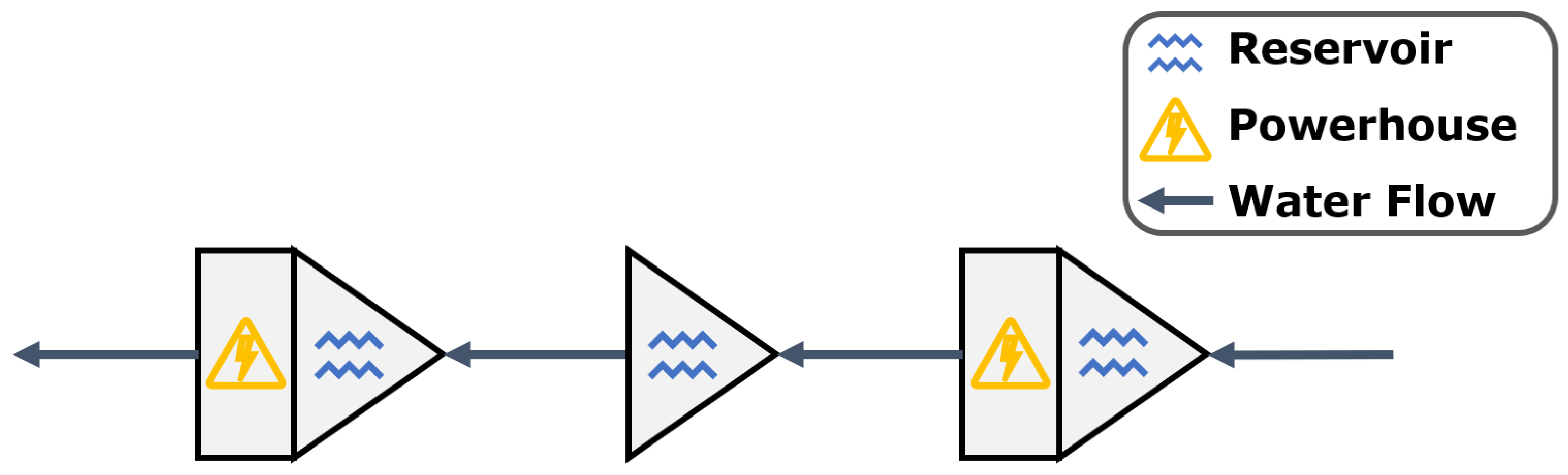
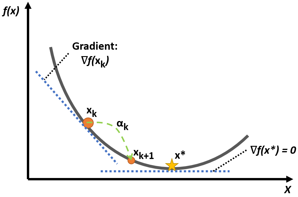