The Scheduling Research of a Wind-Solar-Hydro Hybrid System Based on a Sand-Table Deduction Model at Ultra-Short-Term Scales

Abstract

Establishing a wind-solar-hydro hybrid generation system is an effective way of ensuring the smooth passage of clean energy into the grid, and its related scheduling research is a complex and real-time optimization problem. Compared with the traditional scheduling method, this research investigates and improves the accuracy of the scheduling model and the flexibility of the scheduling strategy. The paper innovatively introduces a sand-table deduction model and designs a real-time adaptive scheduling algorithm to evaluate the source-load matching capability of the hybrid wind-solar-hydro system at ultra-short-term scales, and verifies it through arithmetic examples. The results show that the proposed adaptive sand-table scheduling model can reflect the actual output characteristics of the hybrid wind-solar-hydro system, track the load curve, and suppress the fluctuation of wind and solar energy, with good source-load matching capability.

1. Introduction

The development and utilization of clean energy such as hydro, wind, and solar power are considered key solutions to solve the climate problem [1] and achieving carbon neutrality because of their renewable and non-polluting characteristics [2]. However, wind and solar power generation are random in nature, its transient fluctuations are strong, causing a significant impact on the grid [3], so multi-energy complementary development is needed to suppress the fluctuation of wind and solar power output and ensure the stability of feed-in power [4]. Hydraulic turbines can regulate runoff, and the sensitivity of the unit to stop and start, increase or decrease load is high, making them the optimal complementary energy source for wind and solar multi-energy development [5]. Therefore, establishing a wind-solar-hydro hybrid renewable energy system (HRES) is an effective way of ensuring the smooth passage of clean energy into the grid [6].

Global electricity demand has grown rapidly in recent decades, on the power demand side, the load peak-to-valley differential grows rapidly during peak periods, posing a whole new challenge to the peak-regulation capability of the grid; on the power supply side, as wind and solar enter the grid in large quantities, their inherent volatility, anti-peak regulation, and fluctuation exacerbate the uncertainty of power supply [7]. Therefore, grid security during peak periods has become the main conflict in HRES operation [8]. In HRES, hydropower is responsible for tracking the load curve and regulating the fluctuation of solar and wind power, so the research of source-load matching scheduling for hydropower has become a key issue for the smooth passage of HRES into the network [9].

Previous scholars have conducted extensive research on source-load matching scheduling strategies for HRES. Uddin et al. [10] enumerated different techniques for a hybrid system scheduling method and discussed their operation and control methods in detail. Li et al. [11] constructed a hybrid clean energy microgrid and a two-tier dispatch model for use in a scheduling study from an economic perspective. Ma et al. [12] adopted the Mixed Integer Linear Program algorithm in the scheduling research, phased calculating the HRES short-term scheduling strategy. Li et al. [13] proposed an implicit optimal scheduling research framework, which differs from the traditional algorithm-based scheduling research model, and undertook short-term scheduling research in the form of building a library of operational rules. Wang [14] considered the study of scheduling strategy for cooperative wind, and photovoltaic operation with a dual hydraulic turbine, and verified its source-load matching capability with arithmetic examples. Further, some scholars consider the stochastic and fluctuating nature of wind and solar power in the HRES scheduling strategy. Diana et al. [15] discussed the influences of the uncertainty of wind and solar energy on an isolated microgrid. Liao et al. [16] modeled the uncertainty of wind and solar output, proposed the HRES short-term scheduling model considering wind and solar risk deviation, and verified the validity of the model using arithmetic examples. Chen et al. [17] solved the problem concerning wind and solar output uncertainty by establishing wind and solar confidence intervals in the scheduling research. Liu et al. [18] analyzed the wind and solar prediction error distribution with kernel density estimation, considering the prediction error as a constraint in the scheduling study.

1.1. Gaps in the Research

Traditional HRES source-load matching scheduling research is usually based on a short-term scheduling model, which calculates the next-day scheduling strategy for hydropower according to certain objective functions and constraints based on the day-ahead forecasts parameter of wind, solar, and load; however, engineers using the short-term scheduling research model face difficulties when trying to solve the following problems:

• Model input: The HRES scheduling models input parameters such as wind speed and solar radiation intensity are usually based on short-term prediction models, which type of model has some error due to the long prediction time, resulting in errors between the scheduling model and the actual peak-shaving demand, and the reference of hydropower scheduling strategy seeking results is weak.
• Model construction: the wind, solar, and hydro power output in the short-term scheduling model is usually measured by empirical formulae, which is difficult to apply to all types of wind and solar power units, and cannot describe the process of unit output, which may lead to errors in the measured values of wind, solar and hydro output.
• Scheduling method: in the HRES short-term scheduling model, hydropower operates on an hourly scale peaking on the following day according to the previous day’s scheduling-seeking strategy, while wind, solar power, and load actually show minute-scale fluctuations, and the lack of flexibility in hydropower peaking leads to the scheduling model’s inability to achieve source-load matching.

1.2. Motivation and Contribution

According to the aforementioned gaps in the research, in the HRES short-term scheduling study, there are problems of insufficient accuracy of scheduling models and poor flexibility of scheduling strategies in the HRES short-term scheduling study. In the present HRES scheduling research, the method of hybrid system scheduling under the ultra-short-term scale is proposed. The ultra-short-term scheduling is characterized by capturing peaking demand in real-time based on ultra-short-term forecasts of wind, solar, and load with short forecast time and high accuracy, and giving hydropower a quick-peaking signal to ensure that the hybrid system tracks the load curve in real-time. Ultra-short-term scheduling differs from short-term planning scheduling research, which is a complex, real-time, unscheduled, stochastic optimization problem that uses a more accurate scheduling model and shortens the scheduling decision time to facilitate source-load matching by HRES. Short-term scheduling models and strategies are inapplicable to ultra-short-term research.

As for the scheduling model, the electricity sand-table deduction model draws on the military-style sand-table simulation, based on the electricity modular simulation model, deducing whether a scheduling method or regulation measures (which can be deemed analogous to war scenarios) is correct, the safe and stable operation of power system is simulated by sand-table deduction model. The model realizes real-time adaptive scheduling of hybrid systems by constructing a power simulation model, making real-time decisions, simulating and evaluating various scheduling schemes according to peak-shaving demand, and finding out feasible hydropower operation strategies. Here, the sand-table deduction model is introduced into the HRES ultra-short-term scheduling study to guide the source-load matching scheduling operation at the ultra-short-term scale.

As for the scheduling strategy, the ultra-short-term scheduling research place higher demands on the timeliness and effectiveness of the scheduling strategy. Therefore, this paper introduces the ultra-short-term real-time adaptive scheduling strategy, which takes source-load matching as the target, automatically detects HRES output in the scheduling model, analyzes peaking demand in real-time, gives rapid peaking signals to hydropower, and guarantees HRES has the ability to track the load curve in real-time at the ultra-short-term scheduling scale. The sand table deduction model and adaptive scheduling algorithm proposed in this paper can solve the following problems:

• Model input: for the wind speed and solar radiation in the input parameters of the scheduling model, replacing short-term forecasts with ultra-short-term forecasts of shorter prediction time and higher accuracy as input, to reduce scheduling model input errors.
• Model construction: building HRES electricity sand-table deduction model to obtain wind, solar, and hydro power output, instead of obtaining output by traditional empirical formulae, effectively reflecting the actual output and change process of each type of energy in HRES.
• Scheduling method: constructing ultra-short-term real-time adaptive scheduling strategy instead of the traditional short-term planned model to give full play to the hydropower peak regulation potential and increase the source-load matching capability of the scheduling model.

The structure of the paper is as follows: Section 1 introduces the overview and methodology of the ultra-short-term scheduling research, Section 2 constructs the ultra-short-term sand-table deduction model and real-time adaptive scheduling strategy, Section 3 summarizes the analysis of some examples, and the conclusions are summarized in Section 4.

2. Methodology

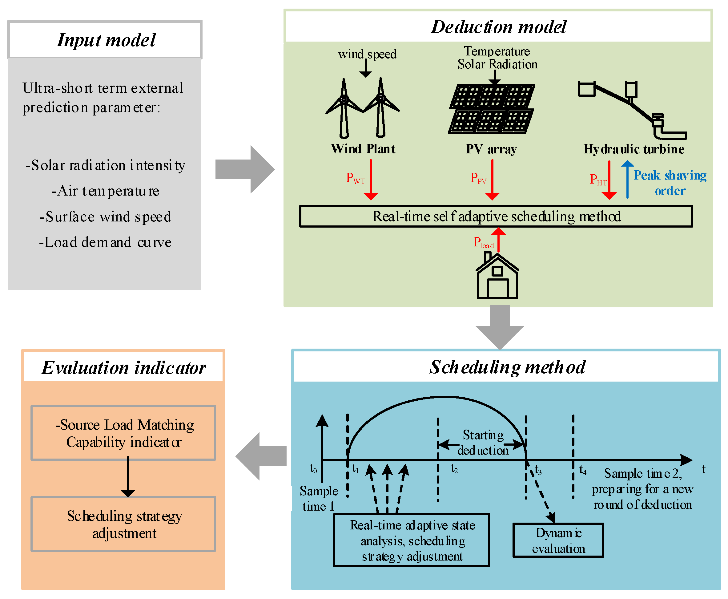
The sand-table deduction model is used to guide the ultra-short-term scheduling operation of HRES, and the constructed sand-table model should reflect the actual output of HRES as far as possible. The sand-table model is shown in Figure 1, including the input model, deduction model, deduction method, and evaluation indicator. Among them, the input model includes the wind, solar, and load ultra-short-term forecast parameters required for the scheduling; the deduction model takes the actual output of the HRES as the modeling target, modular modeling the electric power simulation model of wind, solar, and hydropower. The deduction method is the real-time adaptive scheduling process of the hybrid system, including state analysis, decision adjustment, real-time deduction, and dynamic evaluation. The evaluation indicator is used to assess the results of the HRES deduction output.

The HRES sand-table model-related parameters are listed in

Table 1. Sand-table model-related parameters.

Parameters	Description	S	Solar Radiation Intensity
Wind power		U	Voltage of PV array
PWT	Wind power output	I	Current of PV array
Pr	Wind turbine mechanical power output	Hydro power
Cp	Wind energy utilization	PHT	Hydropower output
ρ	Air density	YPID	Output of the governor
R	Wind wheel radius	Y	Output of the guide vane opening value
V	Wind speed	Ty	Response time constant of the servo-motor
λ	Leaf tip speed ratio	H	Head of water
β	Pitch angle	Q	Flow through the hydraulic turbine
W	Wind wheel rotational speed	hw	Characteristic coefficient of the penstock
Tβ	Time constant (0.2)	Tr	Time constant of the elastic water hammer
τ	Time delay (0.2 s)	Mt	Mechanical torque
βr	Pitch angle setting value	$e_y$	Transfer coefficient of the mechanical torque Mt to the guide vane opening Y.
λopt	Optimal leaf tip speed ratio	$e_h$	Transfer coefficient of the mechanical torque Mt to the water head H
Solar power		$e_{qh}$	Transfer coefficient of the water flow Q to the head of water H
PPV	Solar power output	X	Rotation speed of the hydraulic turbine
Isc	Short-circuit current (4.75 A)	M	Difference in mechanical torque input by the hydraulic turbine
Voc	Open-circuit voltage (21.75 V)	Ta	Inertia time constant
Im	Current in maximum power point (4.515 A)	en	Comprehensive self-adjusting coefficient
Vm	Voltage in maximum power point (17.25 V)	Evaluation indicator
Tref	Operating temperature	I	Source-load matching indicator
Sref	Solar radiation reference value (1000 W/m2)	$m^i$	Rate of change of the output of the HRES within sampling time i
C1, C2, T1, S1	Intermediate variables	$m_L^i$	Rate of change of the load demands within sampling time i
a, b	Compensation factor (a = 0.0054, b = 0.21)
T	Air temperature

.

2.1. Input Model

The input model consists of the ultra-short-term predictive external parameters required for deduction, including solar radiation intensity, air temperature, surface wind speed, and load demand curve. The forecast data can be obtained from the power plant operating data.

2.2. Deduction Model

The sand-table deduction model is shown in Figure 2, including the electricity simulation model of a wind power generation system, a solar power generation system, and a hydropower generation system, with the goal of reflecting the power output characteristics of each power source for modular modeling.

2.2.1. Wind Power System Model

The wind power system model includes multiple turbine units, each consisting of a wind turbine module, a controller module, a pitch module, and a generator module. The input to the wind power system is the ultra-short-term predicted external wind speed and the output is the wind power output P_WT.

(1)

Wind wheel module

The wind wheel module receives wind at speed and converts wind energy into mechanical power output. The relationship between the mechanical power output by the wind wheel and the wind speed is expressed as follows [19]:

$$Pr=Cp\left(\lambda ,\beta \right)0.5\rho \pi R^2{V}_{}^3$$

(1)

The following equation is used to calculate the wind energy utilization coefficient Cp [20]:

$$\begin{array}{l}Cp=Cp(\beta ,\lambda )=0.22[\frac{116}{{\lambda }_i}-0.4\beta -5]e^{-\frac{12.5}{{\lambda }_i}}\\ \frac{1}{{\lambda }_i}=\frac{1}{\lambda +0.08\beta }-\frac{0.035}{{\beta }^3+1}\end{array}$$

(2)

To calculate the wind energy utilization rate Cp, the leaf tip speed ratio λ is introduced.

$$\lambda =\frac{WR}{V}$$

(3)

(2)

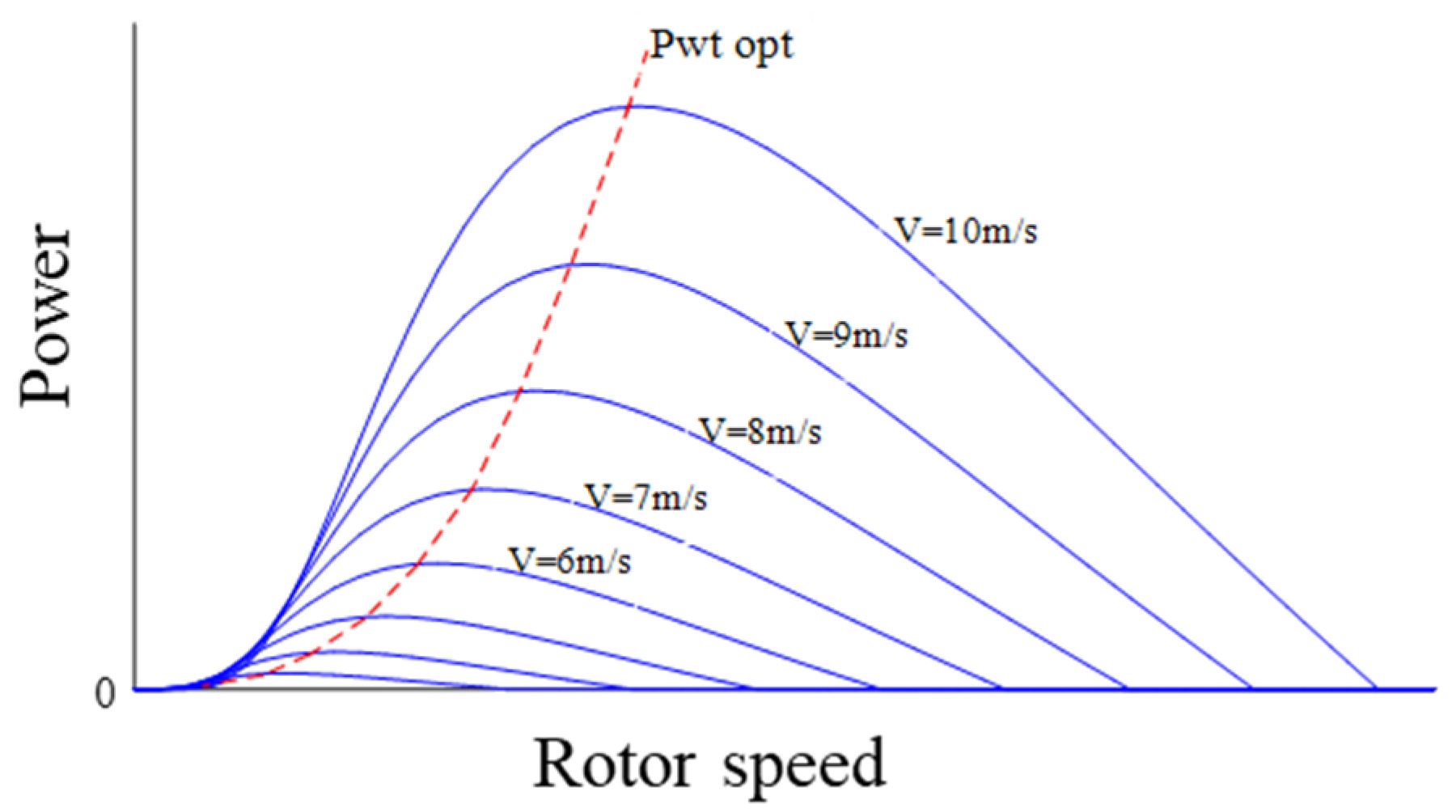
Controller module

The controller module controls the wind turbine status and the amount of mechanical energy output. Due to the non-linearity of wind turbines, the wind speed affects the output of each unit. In accordance with different wind speeds, the controller has two control mechanisms: a variable rotor and a variable pitch angle. The controller modeling process is shown in Appendix A.

(3)

Variable pitch module

A hydraulic driving system in the variable pitch model of large-scale wind turbines is simulated with an inertial system with delay. The transfer coefficient is expressed as follows:

$$\frac{\beta \left(s\right)}{{\beta }_r\left(s\right)}=\frac{1}{T_{\beta }s+1}{e}^{-\tau s}$$

(4)

(4)

Generator module

The generator can convert mechanical energy into electrical output, usually a permanent magnet synchronous generator. Since the permanent magnet synchronous turbine has no gearbox, the turbine drive shaft is connected to the generator rotor, and the transmission loss is negligible.

2.2.2. Solar Power System Model

The solar power system model consists of a PV array: a practical PV array model is therefore adopted in the present research. The solar power system input is the ultra-short-term predicted solar radiation intensity and temperature, and its output is P_PV.

(1)

PV array module

In this section, the mathematical expressions of the simulation model of a PV array are obtained as follows (Equation (5)) [21]:

$$\begin{array}{l}{C}_1=\left(1-\frac{I_m}{I_{sc}}\right)\exp \left(-\frac{V_m}{C_2{V}_{oc}}\right)\\ C_2=\left(\frac{V_m}{V_{oc}}-1\right)/In\left(1-\frac{I_m}{I_{sc}}\right)\\ T_1=T-T_{ref}\\ S_1=\frac{S}{S_{ref}}-1\\ D=I_{sc}{S}_1+a{T}_1\left(1+S_1\right)\\ dv=b{T}_1+D{R}_s\\ I=I_{sc}\left\{1-C_1\left[1-\exp \left(\frac{V+dv}{C_2{V}_{oc}}\right)\right]\right\}+D\\ P_{pv}=UI\end{array}$$

(5)

(2)

Maximum power capture module

The maximum power capture module ensures that the PV achieves maximum power capture, usually using the constant voltage tracking method. When the solar radiation is greater than a certain value and the temperature does not change much, the maximum power point of the PV array is almost distributed near the two sides of a vertical line, and the PV array output voltage is controlled at a certain voltage near its maximum power point, the PV array will obtain the approximate maximum power output.

2.2.3. Hydropower System Model

A hydropower system is usually a mixed-flow hydraulic turbine, including a governor, an electro-hydraulic servo system, a pressure penstock, and a hydraulic turbine. The hydraulic turbine is used to adjust the output P_HT according to the peak-shaving signal value.

(1)

Governing system module

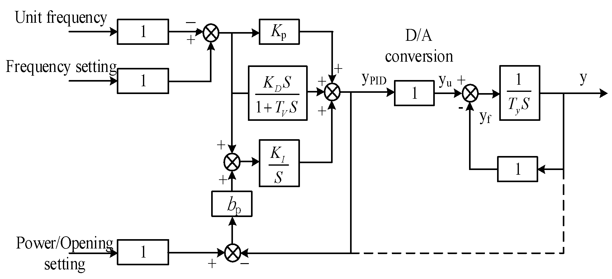
The governor is the core of the stable operation of the hydro turbine, which receives the peak shaving signal and converts it into a suitable output power setting to realize peak regulation operation. The PID-type microcomputer-based controller is usually adopted and its principle of operation is shown in Figure 3 [22]. The controller inputs the output power setting value and outputs the appropriate guide vane opening angle y.

(2)

Electro-hydraulic servo system module

In the dynamic process of large fluctuations in engineering practice, the transfer function of the linear part of the hydraulic turbine servo-motor system is expressed in Equation (6) [23].

$$G\left(s\right)=\frac{Y(s)}{Y_{PID}(s)}=\frac{1}{T_{y}s+1}$$

(6)

(3)

Pressure penstock and hydraulic turbine module

The transfer function of the pressure penstock system considering the effect of the elastic water hammer is given by Equation (7) [24].

$$G_h(s)=\frac{H(s)}{Q(s)}=-h_w\frac{T_{r}s+\frac{1}{24}{T}_r{}^3{s}^3}{1+\frac{1}{8}{T}_r{}^2{s}^2}$$

(7)

The transfer function of hydro-turbine can be written as Equation (8) [25].

$$G_t(s)=\frac{M_t(s)}{Y(s)}=e_y\frac{1+e_h{G}_h(s)}{1-e_{qh}{G}_h(s)}$$

(8)

According to Equations (7) and (8), the hydraulic turbine is modeled by considering the effect of the elastic water hammer on the pressure penstock, as follows:

$$G_t(s)=e_y\frac{24-24e_h{h}_w{T}_{r}s+3T_r^2{s}^2-e_h{h}_w{T}_r^3{s}^3}{24+24e_{qh}{h}_w{T}_{r}s+3T_r^2{s}^2+e_{qh}{h}_w{T}_r^3{s}^3}$$

(9)

2.3. Scheduling Method

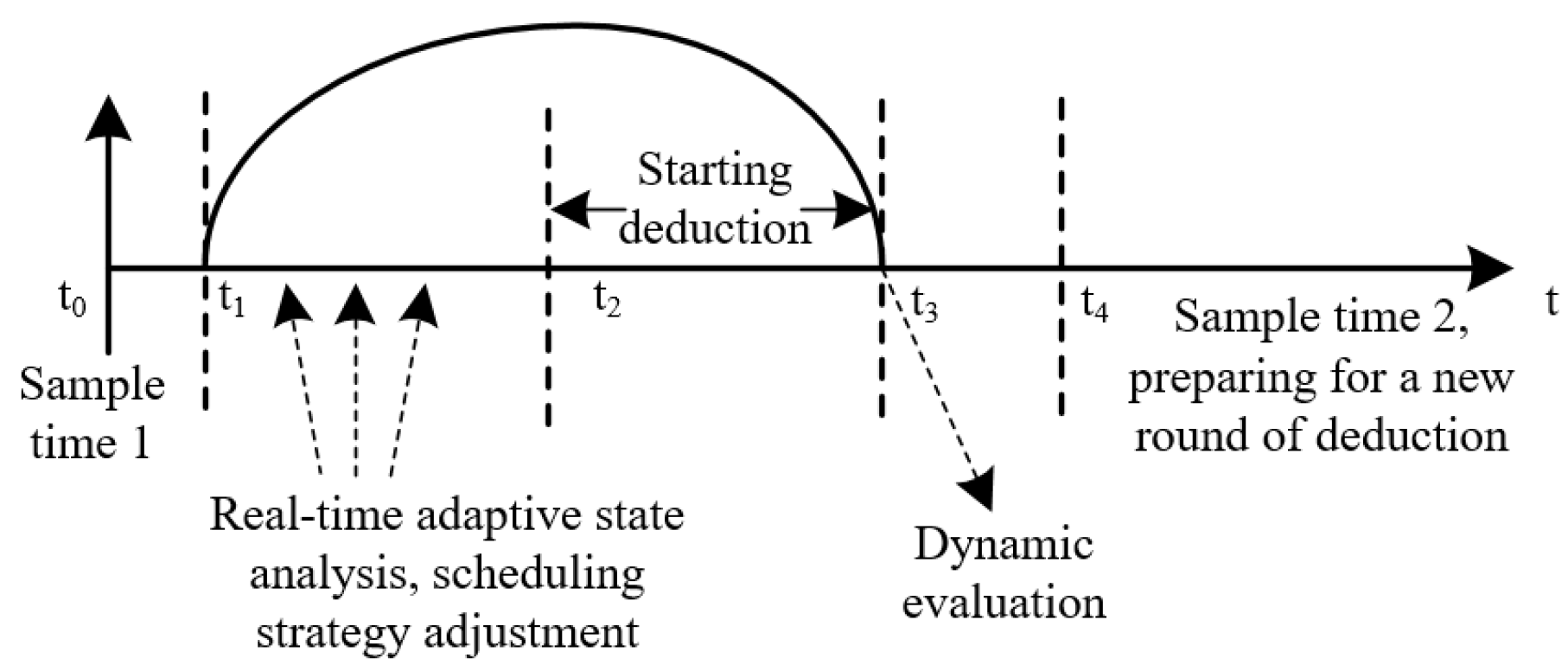
The scheduling method takes real-time source-load matching as the target, which enables HRES to achieve adaptive peaking capability according to the output and load demand deduced from the ultra-short-term scheduling model in real-time, and the scheduling strategy method is shown in Figure 4. During any sampling interval, in the t₁ period detecting the peaking demand in real-time, and generating the hydropower peaking strategy automatically; in the t₂ period adopting the hydropower peaking strategy within the sand table model for rapid deduction, obtain the HRES output, in the t₃ period performing dynamic evaluation for HRES output; then repeating steps t₁, t₂, and t₃ and adjust the hydropower peaking strategy, until the hybrid system model output meets the peaking demand, and then outputs the hydropower peaking strategy.

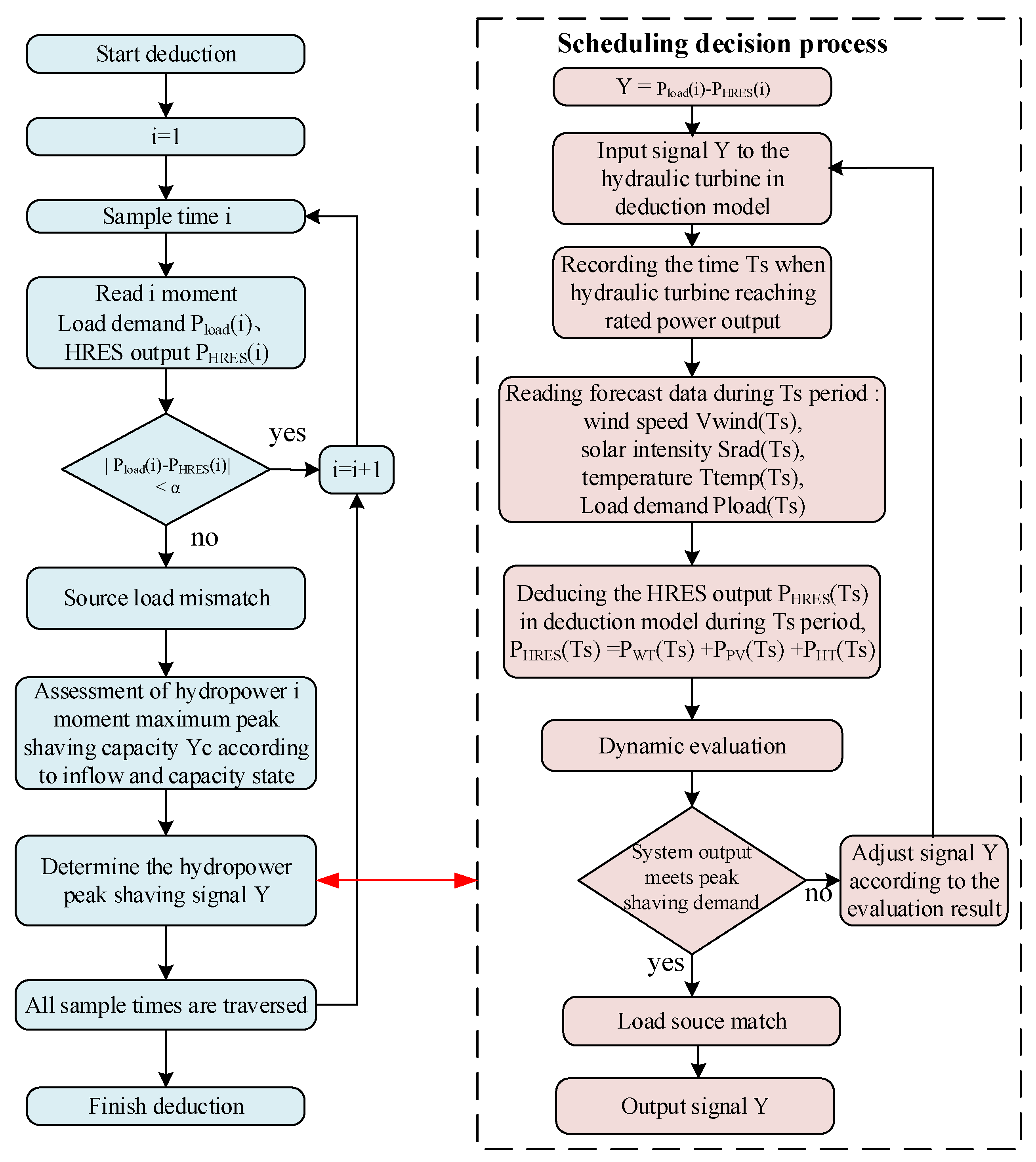
Based on the above scheduling strategy method, the flow of the ultra-short-term real-time adaptive scheduling algorithm is illustrated in Figure 5.

The ultra-short-term real-time adaptive scheduling method proceeds as follows:

Step 1: The source-load matching degree of the HRES at sampling time I is analyzed and the difference between HRES output and load demand at time i is calculated. If the difference satisfies the maximum allowable power supply difference α of the grid, the source load matches, wait until time (i + 1) to sample and analyze the data again; otherwise, the source load does not match, so then, the maximum peaking capacity of hydropower is evaluated at this time, and prepared for the deduction;

Step 2: the hydropower peaking strategy is determined according to the hydropower peaking capacity and the actual peaking demand at time i and the peaking signal Y to hydropower is delivered in the deduction model. Then the time T_s used for stabilizing the hydropower output to the power value set in the peaking strategy is evaluated. The wind speed, solar radiation, temperature, and load demand ultra-short-term prediction values during T_s are read and the sand-table model is used to deduce and measure the wind, solar, and hydropower output during T_s.

Step 3: the load demand and HRES output during T_s are determined according to the previous deduction and the source-load matching degree of HRES is dynamically evaluated, and if the evaluation requirements are satisfied, then jump out of the loop in the deduction model and output the hydropower peak-shaving signal Y; if not, the peaking signal Y is adjusted and the sand-table deduction and dynamic evaluation are conducted again.

2.4. Evaluation Indicator

The dynamic evaluation indicator considers the HRES source-load matching capability. The time taken to stabilize the hydropower output to the power value set by the peak-shaving strategy in the scheduling model is assumed to be T_s. The source-load matching indicator is expressed as follows:

$$\min I=\frac{1}{T\mathrm{s}}{\displaystyle \sum _{i=1}^{T\mathrm{s}}|m^i-m_L^i|}$$

(10)

3. A Case Study

3.1. Model Input

Taking the clean-energy base in the upper Yellow River Basin of China as the research object, the region is rich in wind, solar, and hydropower resources, providing favorable conditions for the construction of a large hybrid clean-energy base, with 2000 MW of wind power, 4000 MW of solar power, and 4160 MW of hydropower planned therein. In the present research, a wind farm (100 MW), a photovoltaic plant (50 MW), and a hydro turbine (250 MW under planning) in the region with similar distances between them are taken as an example to build an HRES sand-table deduction model and conduct an ultra-short-term source-load matching scheduling study; the key parameters of the HRES model are listed in

Table 2. Parameters of HRES model in the examples.

Type	Parameter	Unit	Value
Wind power	Total installed capacity	MW	100
	Installed capacity of turbine	MW	2.5
	Number	set	40
	Hub height	m	90
	Rotor diameter	m	121
	Vcut-in	m/s	3
	Vcut-out	m/s	22
	Vrated	m/s	10
	Rated generator speed	rpm	13.5
Solar power	Total installed capacity	MW	50
	Short-circuit current	A	4.75
	Open-circuit voltage	V	21.75
	Current at the maximum power point	A	4.515
	Voltage at the maximum power point	V	17.25
Hydropower	Installed capacity (design)	MW	250
	Normal water level (design)	m	645
	Usable storage (design)	108 m3	4.776

(wherein the required parameters and operating data were obtained from China Hua’neng Dingbian Renewable Energy Power Generation Company).

Herein, the HRES sand-table deduction model includes a wind power plant, a photovoltaic station, and a hydraulic turbine. The total installed capacity of the wind power plant is 100 MW, including 40 wind turbines with 2.5-MW permanent magnet synchronous turbines; the total installed capacity of the photovoltaic plant is 50 MW, using monocrystalline silicon photovoltaic modules; and the hydraulic turbine is a 250 MW mixed-flow turbine.

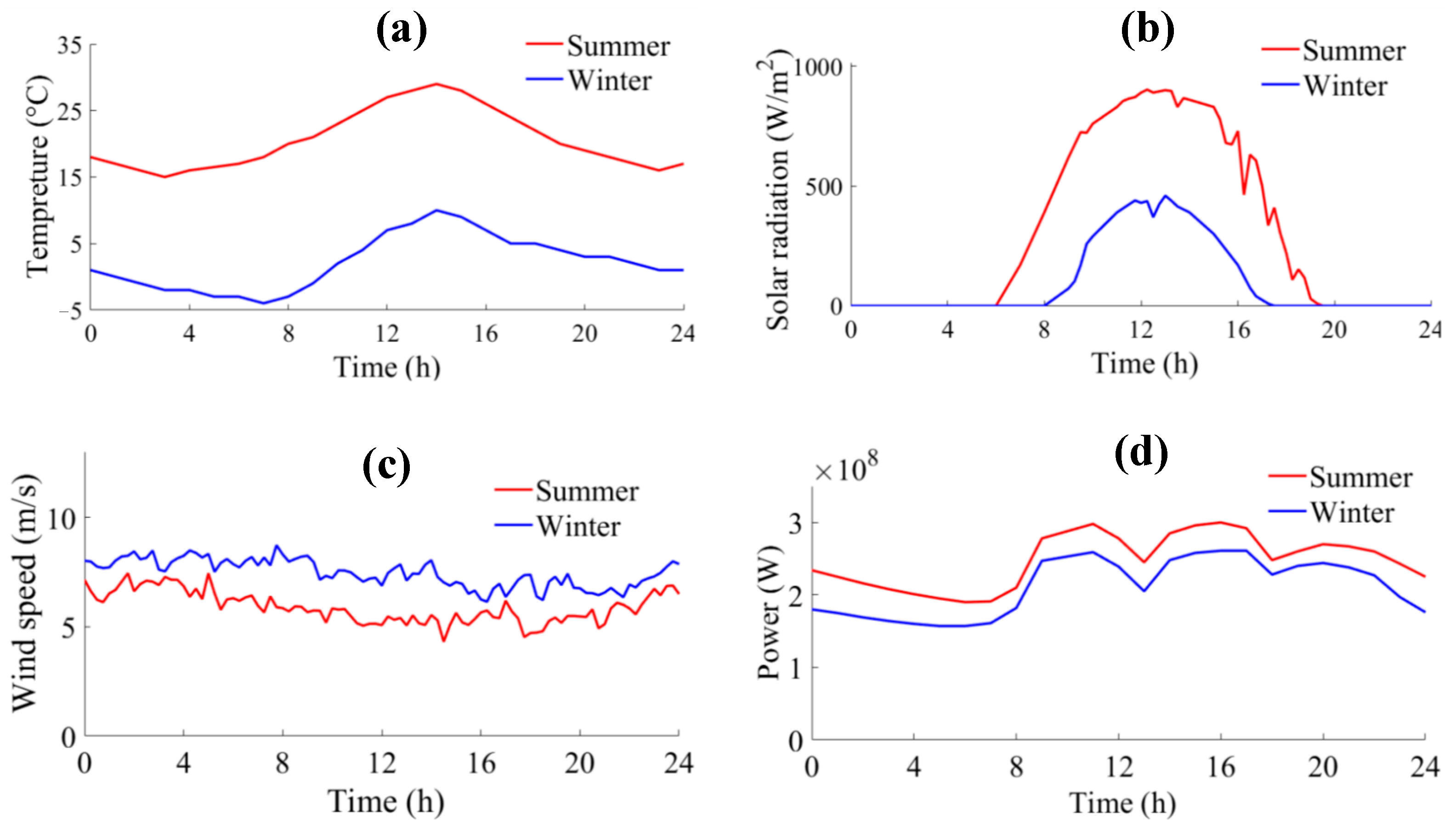
To guarantee the diversity of scheduling deduction results, the HRES ultra-short-term source-load matching scheduling study is carried out on typical days of summer and winter in the example area respectively. The ultra-short-term forecast input parameters required for the deduction include air temperature, solar radiation intensity, surface wind speed, and load demand curve (Figure 6).

As illustrated in Figure 6, the example area is rich in photovoltaic resources in summer and poorer in wind-energy resources; rich in wind-energy resources in winter and poorer in photovoltaic resources; the load demand in summer is greater than that in winter, and the load curves all show three peaks and three valleys.

3.2. Model Construction

To guarantee that the sand-table deduction model proposed herein, as an ultra-short-term scheduling research model, can reflect the real output characteristics of HRES, the validity of the constructed wind, solar, and hydropower models are verified respectively.

3.2.1. Validity Verification of the Solar Model

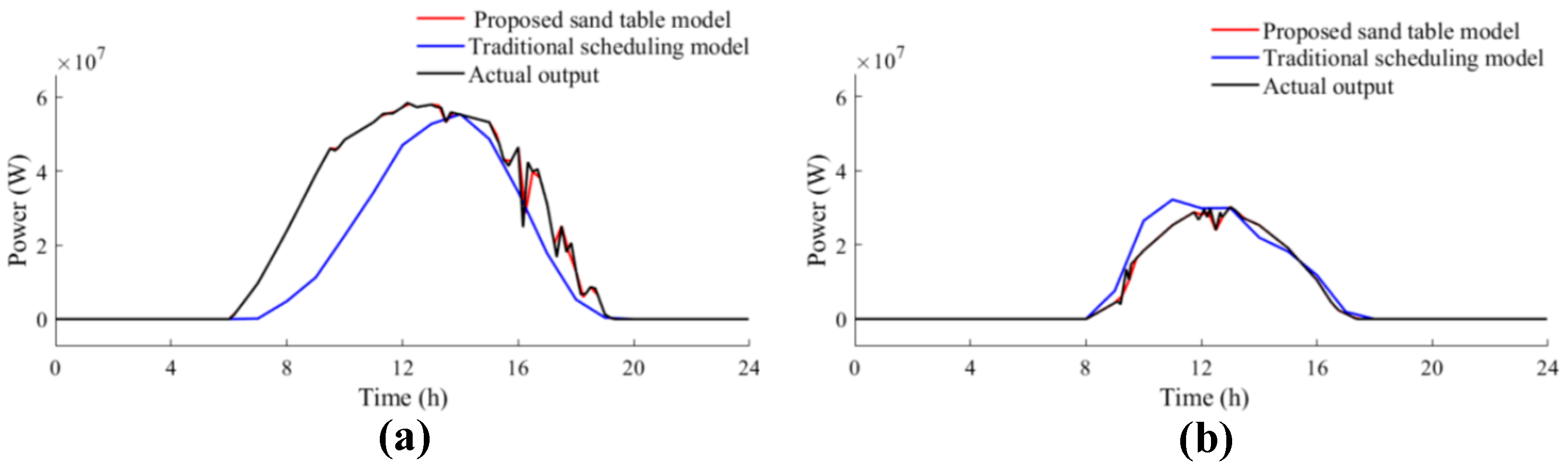
Air temperature and solar radiation intensity ultra-short-term prediction parameters of the example area are input into the solar sand-table model, the deduced ultra-short-term prediction output P_PV is shown in Figure 7. The deduction results are compared with the traditional short-term predicted output and the actual output of solar power.

According to Figure 7, comparing the proposed solar sand-table model (the PV_st model) with the traditional short-term scheduling model, the PV_st model can reflect the fluctuations in solar power due to cloud shading and describe the solar output process more accurately. Since solar models in traditional scheduling studies are usually based on short-term predicted values as inputs and use empirical formulas to calculate photovoltaic output, the proposed method uses ultra-short-term predicted values with shorter prediction time and higher prediction accuracy as inputs and extrapolates photovoltaic output with a more accurate solar sand table model, so the PV_st model better expounds the real output characteristics of solar power.

3.2.2. Validity Verification of Wind Model

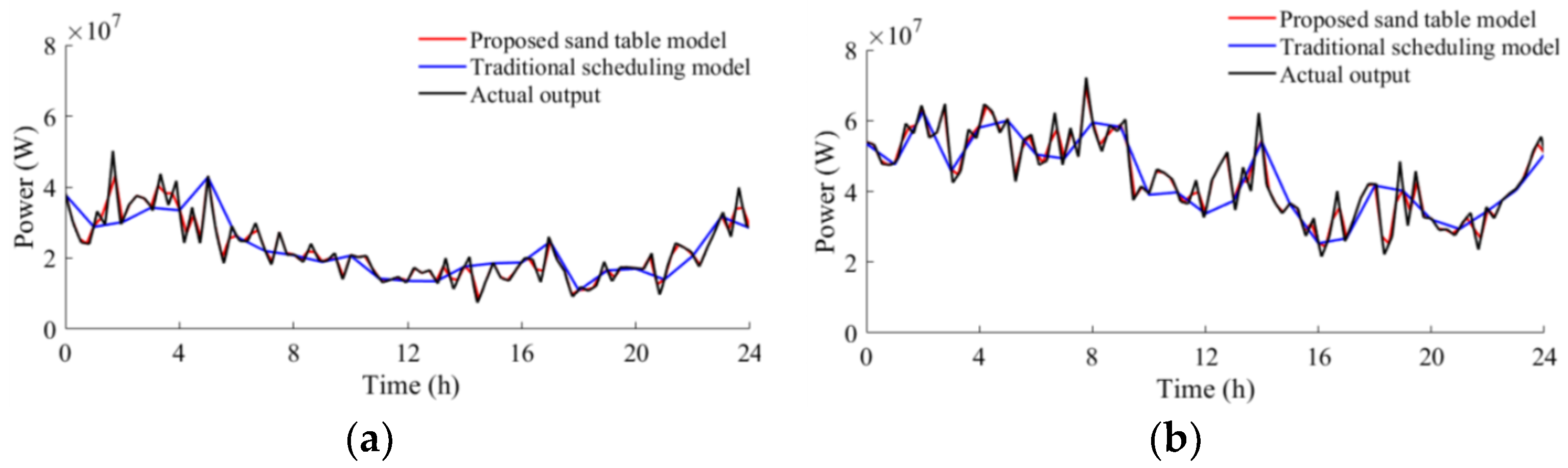
Surface wind speed ultra-short-term prediction parameters of the example area are input into the wind sand-table model, the deduced ultra-short-term prediction output P_WT is as shown in Figure 8: the deduced results are compared with the traditional short-term predicted output and the actual output of wind power.

According to Figure 8, comparing the proposed wind sand-table model (WT_st model) with the traditional short-term prediction model, the WT_st model can reflect the fluctuations in wind power and describe the wind power output more accurately. Since the wind models in traditional scheduling studies are usually based on short-term predicted values as inputs and use empirical formulas to calculate wind power output, the proposed method uses ultra-short-term predicted values with shorter prediction time and higher prediction accuracy as inputs and extrapolates wind power output with a more accurate wind sand table model, so the WT_st model can better reflect the real output characteristics of wind power.

3.2.3. Validity Verification of Hydro Model

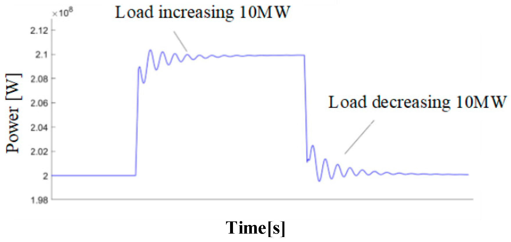
To test the power output characteristics of the hydro sand-table model, when the hydro model runs at the rated power of 200 MW, signals of increasing and decreasing load (using an increment of 10 MW) are input to the governor: Figure 9 shows the change in hydro model output.

Under the action of the controller of the hydropower model, after receiving the signal changing the load by 10 MW, the hydro model rapidly performs a load transition, and its output reaches the pre-set value after fluctuation, only exceeding the scheduled output for a short time, which reflects the highly sensitive power output changes in hydropower load. Therefore, the wind, solar and hydro sand-table model constructed in the present research can reflect the real power output characteristics, and the proposed HRES sand-table model is used as the subsequent ultra-short-term scheduling research model.

3.3. Deduction Results

The ultra-short-term prediction parameters: air temperature, solar radiation intensity, surface wind speed, and load demand curve are input into the HRES sand-table model, and the HRES real-time adaptive scheduling algorithm is used to simulate and deduce the source-load matching capability of HRES on a typical day in summer and winter respectively. The deduced results are shown in Figure 10.

According to the deduction results in Figure 10, the HRES in the calculation example area has good source-load matching capability, during which there is no long-term mismatch between HRES output and load demand. Among them, hydropower can perform adaptive peaking according to load demand and fluctuation of wind and solar, while wind and solar take up certain generation tasks. When the load fluctuation is large, hydropower can quickly increase or decrease the load several times and adjust its output according to the wind and solar fluctuation; when the load fluctuation is small, hydropower increases or decreases the load correspondingly less often. The peak-shaving pressure on hydropower during a typical day in winter is greater than that in summer.

The HRES model in summer and winter has typical daily output characteristics that are similar, and can be unified in any analysis: at 06:00 a load valley occurs; wind power output reached the maximum, the photovoltaic output is 0, the load demand fluctuation in this period of time is small, therefore, the frequency of peak-shaving regulation of hydropower is decreased; at 07:00 to 10:00 and 14:00 to 16:00, the electricity load grows rapidly, the wind power output decreases, the solar output increases and then decreases and reaches the maximum value at around 13:00; hydraulic turbine delivers several load increases for peak regulation. Between 11:00 and 13:00 and 21:00 and 24:00, the electricity load decreases rapidly, the wind power output increases, and the solar output decreases from its maximum value and drops to 0 at around 18:00; the hydraulic turbine performs multiple load-shedding operations for peak regulation. From 17:00 to 20:00, the load demand increases, solar output gradually drops to 0, the wind power output is lower, and hydropower output reaches its maximum.

4. Discussion

According to the ultra-short-term adaptive scheduling algorithm constructed in the present research, the parameter α is the maximum allowable power supply difference, when the difference between HRES output and load demand is greater than α, hydropower must be adjusted to allow ultra-short-term adaptive peaking. The above research only discusses the case where α is 15 MW. It is still necessary to analyze the effects of different values of α on the HRES source-load matching output and find the optimal scheduling value. 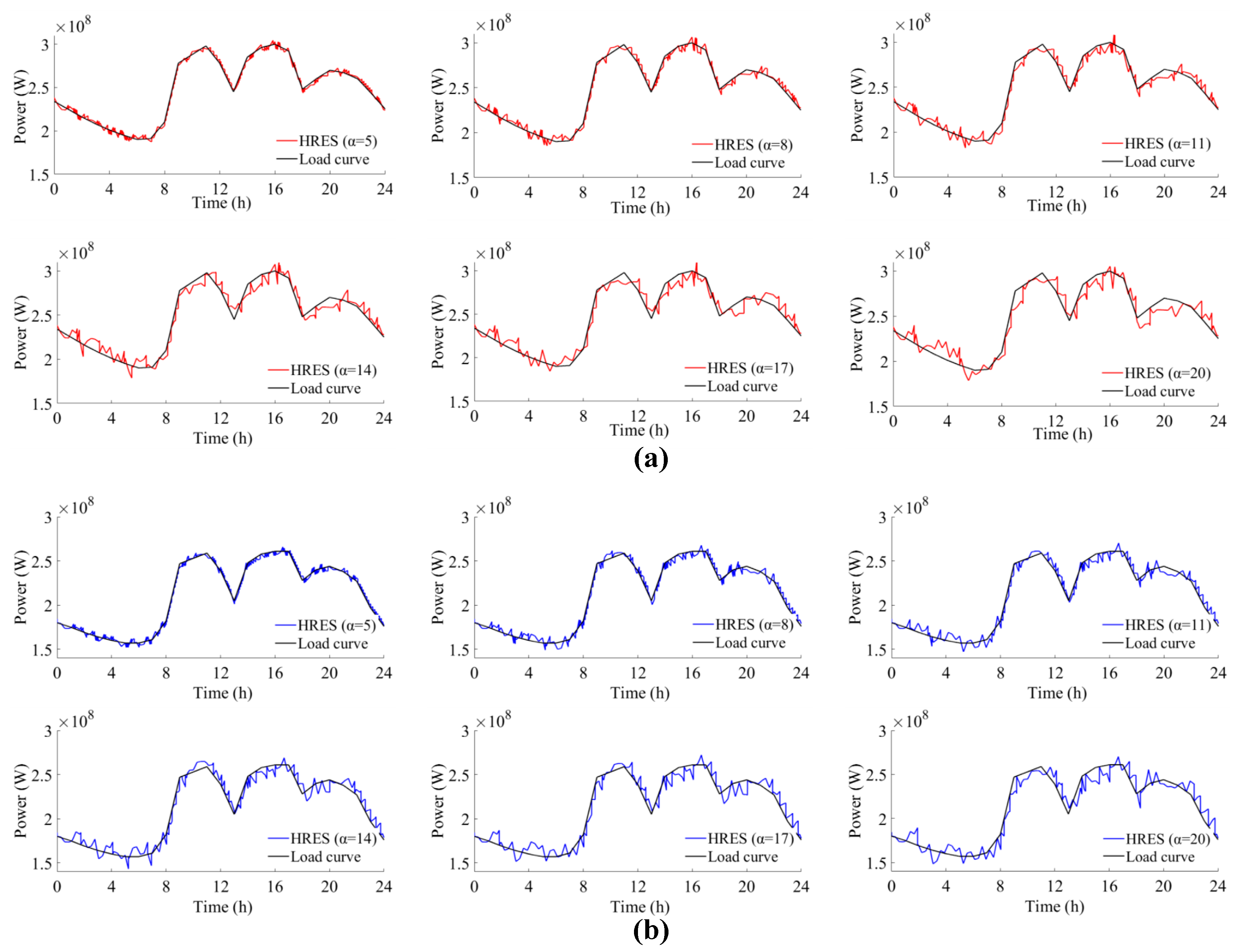For typical summer and winter days in the example area, the HRES source-load matching capability for 16 scheduling scenarios with α values ranging from 5 MW to 20 MW is considered (results are shown in Figure 11).

Figure 11 shows that the smaller the value of α in the adaptive scheduling algorithm, the stronger the overlap between the HRES sand-table model output and the load curve, and the stronger the source-load matching ability; the source-load matching ability of HRES is weaker in winter than in summer. When the value of α is less than 8 MW, the HRES output almost coincides with the load curve; when α is 20 MW, the HRES source-load matching ability is insufficient. Here, considering different values of α, the following indicators are applied to evaluate the source-load matching ability of HRES on typical days in summer and winter in the area of interest (the results of such evaluations are listed in

Table 3. Evaluation results of system output under some α values on a typical summer day.

α	Reliability Indicator (%)	Traceability Indicator	Number of Load Transitions of Hydropower
5	99.45	0.0139	99
8	99.20	0.0134	54
11	98.88	0.0131	34
14	98.48	0.0130	28
17	98.49	0.0119	16
20	98.19	0.0117	14

and

Table 4. Evaluation results of system output under some α values on a typical winter day.

α	Reliability Indicator (%)	Traceability Indicator	Number of Hydro Turbine Load Transitions
5	99.46	0.0165	122
8	99.16	0.0156	66
11	98.91	0.0144	38
14	98.62	0.0142	30
17	98.45	0.0139	22
20	98.23	0.0138	18

).

(1)

Reliability indicator

$$K=1-{\displaystyle \sum _{i=1}^n\left[P_{load}(i)-P_{WT}(i)-P_{PV}(i)-P_{HT}(i)\right]*\frac{100\%}{n}}$$

(11)

where K is the reliability of the system power supply, the larger it is, the stronger the reliability of HRES power output. P_load(i), P_WT(i), P_PV(i), and P_HT(i) indicate the power demand on the load side, wind power output, solar power output, and hydropower output all at time i, respectively; n is the total number of sampling points.

(2)

Traceability indicator

$$I=\frac{1}{n-1}{\displaystyle \sum _{i=1}^{n-1}|m^i-m_L^i|}$$

(12)

where I is the traceability indicator, the smaller it is, the better HRES is able to track the load curve. mⁱ represents the rate of change of HRES output at sampling time i, and $m_L^i$ is the rate of change of load demand in sampling time i.

(3)

Number of load transitions of hydropower

$$\min T={\displaystyle \sum _{i=1}^n{T}_H}$$

(13)

where T and T_H represent the number of load transitions of hydropower within one day and the cumulative number of load transitions of hydropower, respectively.

From the above result, it can be seen that the reliability of HRES becomes weaker after increasing the value of α in the adaptive scheduling algorithm; in terms of traceability indicator, increasing α makes HRES stronger in tracking load, the source-load matching ability increases; in terms of the number of load changes of hydropower, increasing α reduces the number of load changes of hydropower in a given day, the pressure of hydropower peak regulation decreases.

Here, a fuzzy affiliation function is used to calculate the degree of satisfaction for different values of α. That α corresponding to the highest value of satisfaction is the optimal scheduling strategy value, and the satisfaction formula is defined thus:

$${\gamma }_j=\left\{\begin{array}{l}0\hspace{1em}\hspace{1em}\hspace{1em}\hspace{1em}{f}_j(x)=f_j^{\min }\\ \frac{f_j^{\max }-f_j(x)}{f_j^{\max }-f_j^{\min }}\hspace{1em}{f}_j^{\min }\le f_j(x)\le f_j^{\max }\\ 1\hspace{1em}\hspace{1em}\hspace{1em}\hspace{1em}{f}_j(x)=f_j^{\max }\end{array}\right.$$

(14)

where γ_j denotes the degree of satisfaction of the jth objective function; $f_j^{\mathrm{m}\mathrm{a}\mathrm{x}}$ and $f_j^{\mathrm{m}\mathrm{i}\mathrm{n}}$ represent the upper and lower limits of the jth objective, respectively.

The standardized degree of satisfaction is obtained based on Equation (15), and the solution with the largest degree of satisfaction is selected as the optimal scheduling scheme.

$$\gamma =\frac{{\displaystyle \sum {}_{j=1}^M{\lambda }_j}{\gamma }_j}{{\displaystyle \sum {}_{j=1}^M{\lambda }_j}}$$

(15)

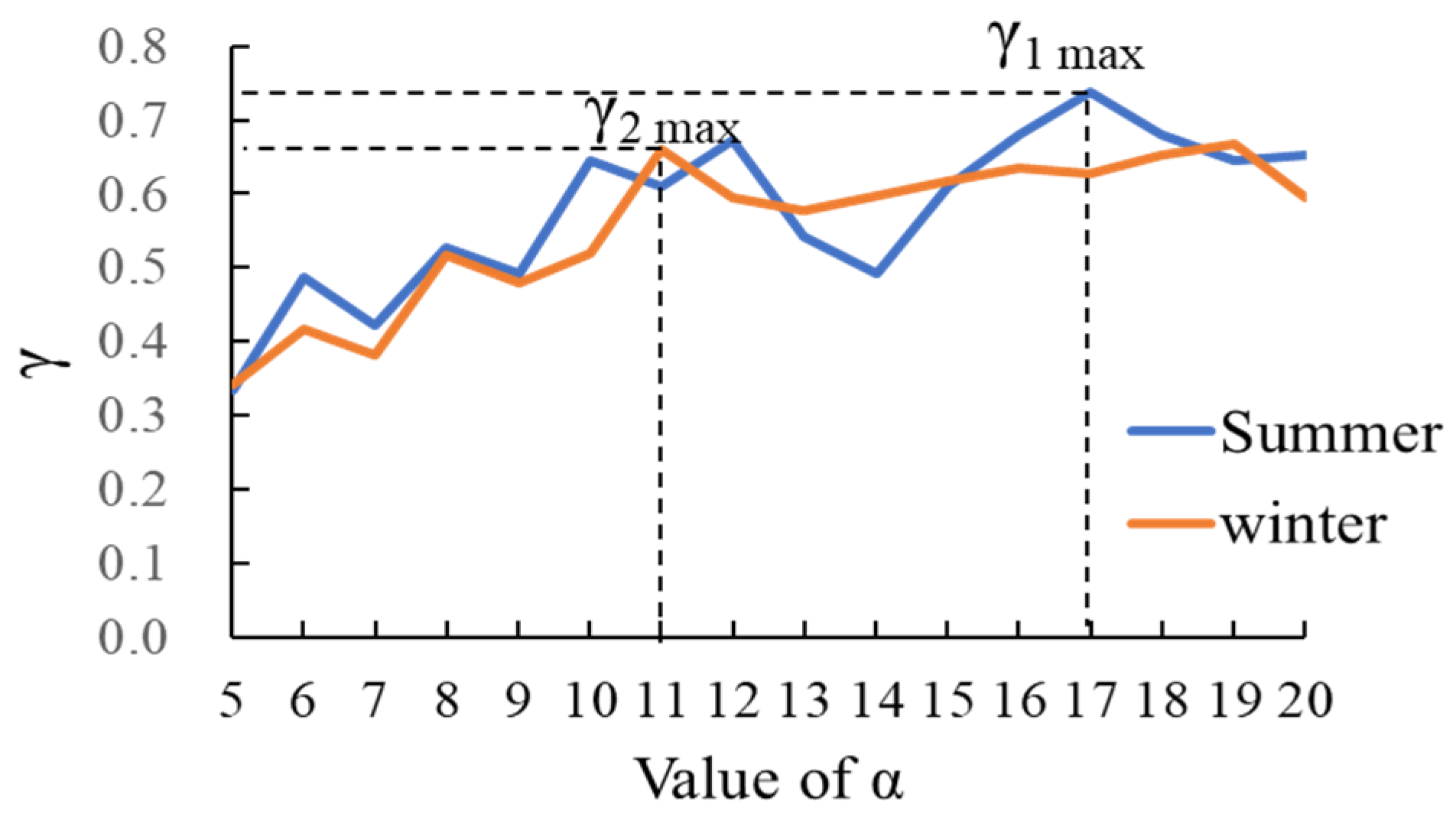
where, γ and λ_j denote the standardized degree of satisfaction and weight of satisfaction of the jth objective, respectively. There are three objective functions in this study, so M = 3. The weights of satisfaction of the three objective functions are equal, that is, λ₁ = λ₂ = λ₃ = 1. Based on the above method, the typical daily γ-values in the interval 5 MW < α < 20 MW for summer and winter are calculated respectively, with 16 values, of which the maximum value is the optimal α value (Figure 12).

As shown in Table 3, for a typical summer day, γ₁ is maximized when α is set to 17 MW in the scheduling algorithm; for a typical winter day, γ₂ is maximized when α is set to 11 MW in the scheduling algorithm, so the reliability of HRES output in summer and winter is optimal when α is set to 17 MW and 11 MW respectively in the area of interest.

5. Conclusions

The present research breaks through the traditional short-term hybrid system scheduling research framework, and examines HRES source-load matching scheduling in terms of reducing scheduling model output errors and enhancing scheduling strategy flexibility, proposing a scheduling research method based on the sand-table deduction model in the ultra-short-term scale, and exploring the scheduling strategy and output characteristics of HRES with hydropower regulation capacity in the ultra-short-term scale, adaptively smoothing wind and solar power fluctuations and tracking load curves. The conclusions are drawn as follows:

• When constructing the wind and solar output prediction model, compared with the traditional short-term prediction model, the accuracy of wind and solar model output prediction can be improved by inputting ultra-short-term prediction parameters and modular modeling of the wind and solar units;
• Based on the proposed real-time adaptive scheduling algorithm, the HRES sand-table model can track the load curve within the ultra-short-term scheduling scale, suppress wind and solar fluctuations, with good source-load matching capability;
• The parameter α is the maximum allowable power supply difference set in the adaptive scheduling algorithm. Increasing α will lead to lower system output reliability, enhanced load tracking ability, and a fewer number of load transitions of hydropower. The reliability of HRES output in summer and winter in the example area is optimal when α is set to 17 MW and 11 MW, respectively.