Article

Second-Life Battery Capacity Estimation and Method Comparison

1
Centre for Renewable Energy Systems Technology, Loughborough University, Loughborough LE11 3TU, UK
2
PowerVault Ltd., Garrick Industrial Centre, Garrick Industrial Estate, Irving Way, London NW9 6AQ, UK
*
Author to whom correspondence should be addressed.
Energies 2023, 16(7), 3244; https://doi.org/10.3390/en16073244
Submission received: 3 March 2023 / Revised: 22 March 2023 / Accepted: 29 March 2023 / Published: 4 April 2023
(This article belongs to the Topic Battery Design and Management)

Abstract

:
There is increased talk about using second-life batteries in applications. In first-life applications, the batteries start from new, and a range of life cycle estimation techniques are applied. However, it is not clear how second-life batteries should be monitored compared to first life batteries. This paper investigated different algorithms from first-life applications for estimating and forecasting battery cell state of health in conjunction with capacity calculations using second life cells under long term durability testing. The paper looks at how close these models predict capacity fade based on a set of second-life batteries that have been undertaking sweat testing over six different applications. The paper concludes that there are two methods that could be suitable candidates for predicting lifespan. One of these needed to be modified from the original.

1. Introduction

With the increase in electric vehicle registrations, there are increasing numbers of used batteries going through the recycling and reuse chain. Once a second-life battery has been graded and sorted, it is possible to reuse it in another application such as stationary storage. There is a significant body of work on tracking capacity fade in new batteries. However, it is not straightforward to establish good ways of tracking remaining life or capacity fade of second-life batteries. This is due to several reasons (details in Table 1):
  • Nearly all the published techniques start with a new battery and assume its end of useful life is 80%, whereas second-life batteries start with an 80% remaining capacity battery [1,2,3]. There are, therefore, very few published records of how batteries degrade below 80% of remaining capacity [4,5,6].
  • The published work uses a variety of different Li-Ion battery chemistries, and what is suitable for one chemistry may not be suitable for others [1,4,7].
  • Nearly all the published data assumed the cycling is from 0% to 100% DOD with no variations. Second-life batteries will undergo different cycling depending on their application and, therefore, they will not be following just a 100% charge/discharge curve. Some of the published methods are adaptable to deal with varying DOD, but it is by no means clear if the adjustments are valid [2].
In this paper, a literature review on published capacity fade methods for first-life applications are reviewed as part of Section 2. Many of these are complicated and require machine learning. Machine learning methods typically require a large amount of training data. The accuracy of the training data is important for the predicted result. Machine-learning-based methods are, therefore, not suitable at this time for second-life batteries where there is a lack of good publicly available data. Section 3, therefore, looks at how the non-machine-learning-based methods can be applied to second-life batteries under long term sweat tests. Section 4 compares the results of the capacity fade estimation using these methods with measured capacity of a set of six second-life batteries on long term test under different sets of cycles.
This work is novel because it investigates using measured data how second-life batteries degrade over time and how this may be estimated using adapted capacity fade techniques.

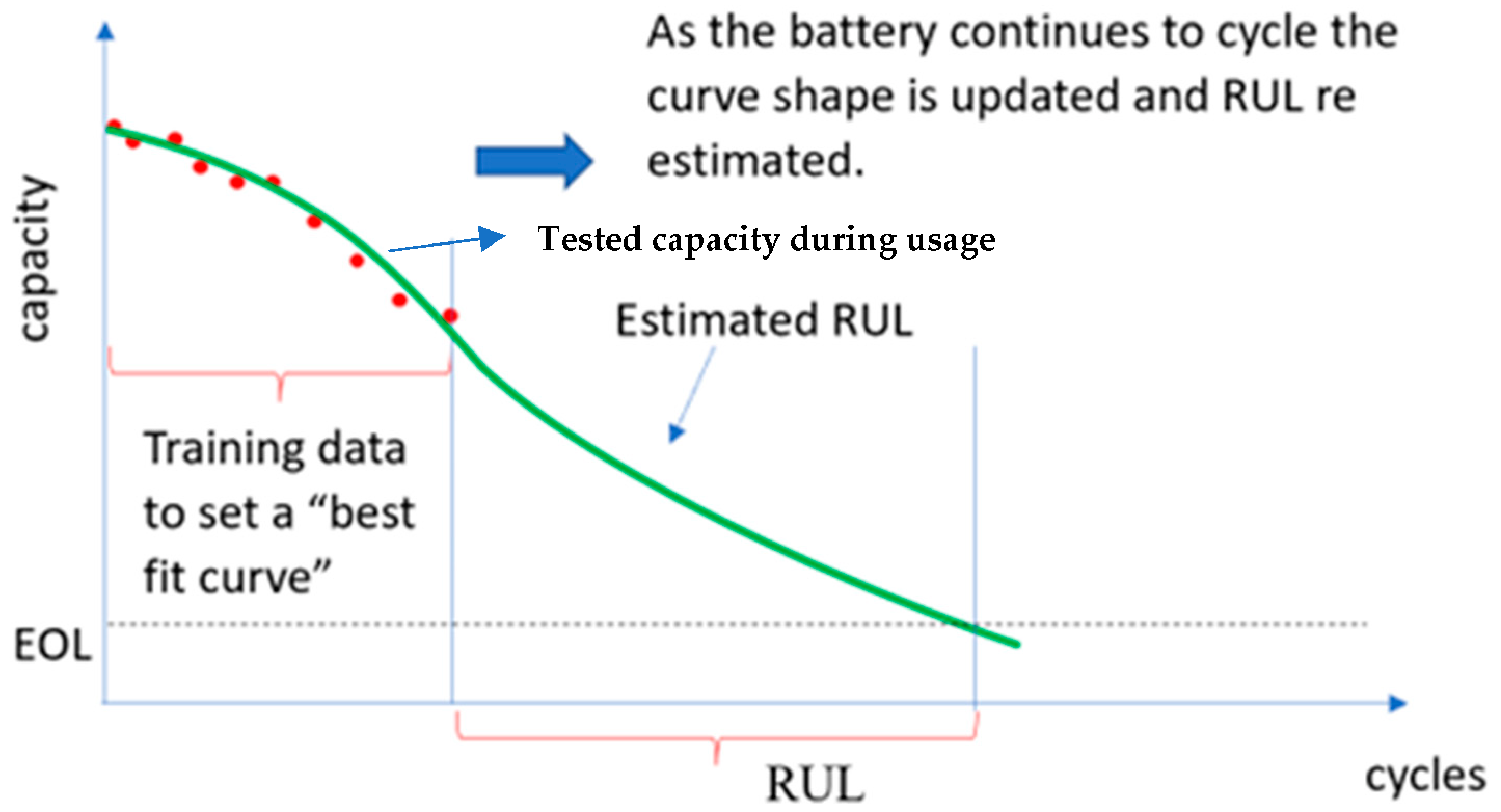
2. Remaining Useful Life Estimation

Life cycle estimation is difficult and is normally based on either capacity or impedance. Most literature uses capacity fade as a key indicator for RUL, while a drop in impedance is typically associated with a power fade.
Batteries undergo a range of different cycles with different rest periods under different rates of charge and discharge at different temperatures. A second-life battery is even more complex because it typically has an unknown history. Many manufacturers produce life cycle curves to act as indicators of the number of cycles that can be expected for a constant depth of discharge. These are typically backed by life cycle testing. The split between calendric (battery resting) and cyclic aging is not always considered with cyclic aging considered more onerous.
This complexity has not stopped the academic community from attempting to come up with imaginative and complex life cycle estimation (or remaining useful life RUL) calculations based on a plethora of information [8,9,10]. It is typical to divide these into model-based methods and data driven methods. Model-based methods require analysis of the degradation mechanism of lithium-ion batteries and depend less on historical data. The electrochemical model or equivalent circuit model are commonly used in current research. Data-driven methods tend to analyze historical data to excavate potential rules, and then apply these rules to predict the development of events. It is not necessary to have a profound knowledge of the degradation mechanism of a battery. The degradation can be predicted by rules derived from historical data. Some of the methods described below can be easily adapted to second-life battery remaining useful life calculations. For example, those that use an empirical formula. Other methods require extensive testing prior to determining algorithms for remaining life or are complex to understand. These are typically based on AI techniques. This paper will only use those methods that are adaptable to second-life batteries without the need for extensive testing.
In many cases, regression is used to adapt constants in empirical equations to track the capacity fade, as shown Figure 1.
There are a variety of different regression techniques used from the least squares fit to a curve [11,12] through to Gaussian process regression [5] and particle swarm optimization regression [3].
The training data can be a measured capacity with time or a health indicator (HI), e.g., time to go from maximum voltage to minimum voltage under a constant current discharge or the shape of the discharge or charge curve [13].
A number of different curve types have been used in previous literature including exponential formula [7,14,15], Polynomial formula [11], the power law [12], and some formulae that are based on empirical examination on test results [1,4].
More complex capacity fade techniques using extensive data training and including AI have been developed and summarized at high level in Figure 2. It is not straightforward to pick up the results and equations within the following methods and, therefore, these cannot be directly used without additional understanding, extensive data set training, and application.
The methods include the Weiner method [16,17,18], support vector machine (SVM) [19,20], which works as shown in Figure 3. The box-cox transformation [6,21], which is a method looks at correlation of data with health indicators.
The majority of these methods are based on AI techniques. The process is, therefore, mostly similar to that described in Figure 2 and does not necessarily rely on battery models to implement. Neural Networks are very popular [22,23,24,25]. There is also a recent skew in literature away from using impedance and capacity to estimate RUL as these are difficult to obtain online. There are many different types of machine learning and curve fitting type methodologies that could be used to solve this problem. Examples include regression fitting of the capacity curve based on relevance vector machine learning and Gray’s model (which works on the differential of the time varying test data) [26], and these can be split into cycle degradation and/or rest time calendric degradation. Other methods use particle filters with other training methods such as neural networks [27] to predict capacity. AI techniques were not applied to the data generated in this paper as the sample size is too small to both train the AI and to generate meaningful results.
The published literature uses a variety of different battery chemistries and sizes to validate the work, but nearly all the tests are undertaken on small cylindrical cells at about 1–2 Ah. A high proportion of tests are also undertaken on pre-established data sets from NASA. Where published, these are included in the review.
Table 1 shows the different chemistries, cycling, or data sets mentioned that have been used by different authors.
Table 1. Key Validation Parameters.
Ref.ChemistryCycling
[1]LiFePO4 in cylindrical packagingCapacity range: 100% to 80% of life
Cycling conditions: Nine batteries with varying temperature, cycle depth, and number of cycles.
[2]LiFePO4 in cylindrical packaging (2.2 Ah)Capacity range: 100% to 80% of life
Cycling conditions: Two batteries under each condition below.
temperature (−30 °C, 0 °C, 15 °C, 25 °C, 45 °C, 60 °C), DOD (90%, 80%, 50%, 20%, 10%) and charge/discharge rate (C/2, 2C, 6C, and 10C)
[4]LiMn2O4 in prismatic package (40 Ah and 80 Ah)Capacity range: 100% to 30% of life
Cycling conditions: Capacity tests with trickle charge rest periods, up to 1600 days testing. Cycle charge/discharge number and process are not clear as the results are in test days only
[7]LiNiCoMnO2 in a cylindrical packageCapacity range: 95% to 75%
Cycling conditions: Two (small) batteries cycled to 100% DOD (with over charge and over discharge to aid degradation) for around 100 cycles. Life estimation based on curve fitting an equation to the data.
[3,5,6,14,16,17,18]LiCoO2Nasa dataset (all or part of) [28]
Capacity range: 100% to 70%
Cycling conditions: Li-ion 18,650 sized rechargeable batteries were cycled to 100% DOD from new to 70% capacity (2 Ah to 1.4 Ah). Life estimation based on curve fitting an equation to the data.
[3,14,16,17]LiCoO2Maryland data set [29]
Capacity range: 100% to 80% capacity range
[15]LiCoO2 (probably)Capacity range: 100–50%
Cycling conditions: Two types of small cells with four of each, full charge and discharge cycle for around 200–800 cycles depending on type.
[11]NiMHCapacity range: 50–0%
Cycling conditions: Two small cells full charge and discharge cycle for around 85 cycles.
[30]Li IonOxford university data set [31]
Cycling conditions: Up to 3600 charging cycles, looking for changes in the incremental capacity data as a function of probability.
[12]LiFePO4Cycling conditions: Four small cells, full charge and discharge cycle for between 363 to 1549 cycles, undertaken during charging above 70% SOC.
[32]LiCoO2Capacity range: 100–70%
Cycling conditions: At least seven small cells at discharge rates of 10% to 90% DOD with up to 4000+ cycles recorded at 50% DOD.
[33]Lithium IonCapacity range: 100%-70%
Cycling conditions: Small cells at 0.5C discharge for 1000 cycles.
[18]Li(NiCoMn)1/3O2Capacity range: 100–80%
Cycling conditions: Six small cells over 840 cycles
undertaken at high temperature to speed aging.
[34]Li(NiCoAl)O2 Panasonic cylindricalCapacity range: 100% to about 60–70%
Cycling conditions: 18 small cells undertaking 100% DOD charge and discharge cycles at cycle rates of 0.5C, 1C, and 2C at different temperatures. Up to 800 cycles recorded.
[22]Lithium IonCapacity range: 100–80%
Cycling conditions: Two small groups of cells, between 2500 cycles, one set with mechanical vibration.
[23]Li(NiCoAl)O2 cylindrical batteriesCapacity range: 100–80% (approx.)
Cycling conditions: 0-100% DOD cycles at different charge rates (1C, 2C and 3.5C) and temperature (25 °C and 40 °C) to around 600 cycles.
For second life applications, it is clear from the data above that many of these methods are appropriate only for small batteries that have capacity faded to 80%. In addition, it is not clear how chemistry impacts the results. Therefore, it is not clear how applicable these methods will be for second life applications.
In addition, many of these methods are complex and require training data that do not exist when the battery enters its second life. Machine-learning-based methods require a large dataset, which is not available. A selection of these methods, described below, have been chosen as possible contenders for determining the capacity fade of a second-life battery on energy storage applications. They were chosen because they do not use extensive training data and are straightforward to implement, thus they can be used in real time.

2.1. Method Used by Swierczynski et al.

Swierczynski et al. [1] proposed two different equations for degradation: power fade and capacity fade. Both power fade and capacity fade are accumulative, and the end of life is chosen as representing the point where these pass 20% capacity degradation. The power degradation is claimed to be lower than the capacity degradation in this paper.
The relevant equations for calendric and cycle power fade and capacity fade are as follows, respectively:
P f a d e = 0.000375 S O C s t + 0.1363 0.155 × 0.003738 t e 0.06778 T
where:
  • P f a d e is the estimate of power fade (calendric);
  • S O C s t is the state of charge the battery is stored at (%);
  • T is the temperature of storage in °C;
  • t is the storage time;
C f a d e = 0.019 S O C s t 0.823 + 0.5195 × 3.258 × 10 9 T 5.087 + 0.295 × t 0.8
where:
  • C f a d e is the capacity fade (calendric);
P f a d e = 1 3 5.78 x 10 4 × e 0.03 T + 1.22 × 10 7 × 2.918 x 10 5 × e 0.08657 c d × n c 0.00434 T 0.008 c d 0.1504
where:
  • P f a d e is the estimate of power fade (cyclic);
  • c d is the cycle depth (%);
  • nc is the number of cycles;
C f a d e = 0.00024 e 0.02717 T × 0.02982 c d 0.4904 × n c 0.5
where:
  • C f a d e is the capacity fade (cyclic).
Figure 4 shows the process involved in implementing this methodology.
Equation (4) relies on cd—the cycle depth (%)—and nc—the number of cycles. The average cd is calculated over nc and used in the equation with equivalent nc, as the original equation relies on fixed cycle depths.

2.2. Method Used by Wang et al.

Wang et al. [2] use a method that fits experimental data to a power law.
Q l o s s = B e E a R T A h z
where:
  • Q l o s s , is the percentage of capacity loss;
  • B is the pre-exponential factor;
  • Ea is the activation energy in J mol−1;
  • R is the gas constant;
  • T is the temperature in Kelvin;
  • Ah is the Ah throughput, which is expressed as Ah = (cycle number) × (DOD) × (full cell capacity), and z is the power law factor.
The experimental data were fitted to give:
Q l o s s = 30 , 330 e 31 , 500 8.314 T A h 0.552
At C/2.
Additionally, generalized to:
Q l o s s = B e 31700 + 370.3 × C r a t e R T A h 0.552
where Crate is the charge rate, B = 31,630 at C/2, 21,681 at 2C, 12,934 at 6C, and 10,512 at 10C.
The Wang method is an exponential curve based on the variable Ah = (cycle number) × (DOD) × (full cell capacity). To deal with degradation at each cycle, the average DOD up to that cycle number multiplied by the number of cycles is used along with the original cell capacity. As the DOD changes each cycle, the average DOD changes between each calculation and it can look as if the battery has recovered between cycles. However, this is just an artefact of the mathematics and should be treated as low level noise.

2.3. Method Used by Matsushima et al.

Matsushima et al. [4] look to represent capacity fade by a time factor:
Q l o s s = K f × t 1 / 2
where:
  • K f is the rate constant;
  • t is time to reach 70% capacity;
  • K f correlates with temperature and satisfies the relationship for cells between 100–70% degradation;
l n K f = 4.2388 × 1000 × T 1 + 13.78
where:
  • K f is the rate constant;
  • T is temperature in K.
For cells below 70% degradation the following equations can be stated to be used to estimated capacity drop.
Q l o s s = 0.9481 t 1 2 + 88.338   @   45 ° C Q l o s s = 1.2906 t 1 2 + 89.746   @   55 ° C Q l o s s = 1.7374 t 1 2 + 91.378   @   60 ° C  

2.4. Method Used by He et al.

He et al. [15] used an exponential curve fitting method. There are a number of exponential curve fitting methods [4,5,6], but this one had the parameters used clearly stated.
The relevant curve fitted equations are as follows:
C k = ae bk + ce dk  
where:
  • C k is the capacity at the kth cycle.
The parameters a, b, c, and d are set from experimental data using different numbers of cycles.
The variables in the equation vary with time but not significantly up to the 60-cycle test that was used. The method in the paper works by estimating these four parameters and using these to estimate the capacity until a fixed end of life criteria is reached. As this does not include depth of discharge as a parameter, it is unlikely to be useful for the second-life battery application in its current form.
The LiCoO2 batteries used by He et al. [15] start with the following:
A = −0.000222, b = 0.04772, c = 0.89767, and d = −0.00094
These values are then adjusted using regression.
The original data set was based on full charging and discharging cycles. This work has been modified so that the exponential curve is based on the varying cycle DOD that is in each cycle multiplied by the scaling factor y2. A starting offset (y1 = 0.76) was added as well as the impact of variable DOD (three values were tried y2 = 1/10, 1/3.9, and 1/1.5).
Equation (11) has been adapted as shown in Figure 5 to deal with partial SOC cycling as follows:
C k = y 1 a e b y 2 k + c e d y 2 k

2.5. Method Used by Dogger et al.

Dogger et al. [32] used test data to establish a parameter called 100% DOD cycle equivalent (DoDCE), as illustrated in Figure 6. There are a higher number of cycles available at a lower depth of discharge than would be achieved by looking at the equivalent energy balance. This can be found from a graphical representation.
If it is assumed, for example, that a first life battery undertakes an average 35% DOD and an estimated 2000 total cycles over 10 years [35], then this equates from the equation below to a DoDCE of 0.35 × 2000 = 700 DoDCE cycles. This can be subtracted from the starting point to give a new starting point for second life applications.
D o D C E = N c y c l e s × D O D  
The process can be continued until DoDCE = 0 using the process in Figure 7:

3. Cycle Testing

The second life cells that were available for testing were two cells in series with two cells in parallel and the operating voltage range was given as:
  • Min cell voltage 5 V/module
  • Nominal cell voltage 7.5 V/module
  • Max cell voltage 8.3 V/module
  • Capacity at new 66 Ah
Within the test cycle as part of the discharge cycle after a CC-CV charge by integrating current with time. [36]
Q = I t d t  
where:
  • Q is the charge being estimated in Ah;
  • I is the discharging current in A;
  • T is discharging time in hour.
A is the number of these batteries that have been on long term sweat tests. The cycles are based on six different second life applications [37]. These are as follows:
  • A house with four people and a solar panel using the battery to absorb extra energy when the PV panel is producing more power than is absorbed in the house, releasing this energy afterwards.
  • A house with four people and PV panels on a time-of-use tariff, where the battery is used to absorb extra energy from the PV panel and release this when the tariff is highest.
  • A house with four people and no PV on a time-of-use tariff—where the battery is charged at low tariff and discharged on high tariff.
  • The battery is operating as part of an aggregated static frequency response system performing on the UK Fast Frequency Response (FFR) market.
  • The battery is operating as part of an aggregated dynamic frequency response system performing on the UK Enhanced Frequency Response (EFR) market.
  • The battery is operating as part of an aggregated system looking to compete in the day ahead market.
The sweat tests did not include sophisticated demand side management or fast charging of electric vehicles in these use cases, as these were not market ready when the testing started. Similarly, microgrid functionality was not included for the same reason. Grid scale peak load lopping was also not included, as there is no market mechanism for dealing with this type of energy storage benefit.
There are some additional electricity markets that are open to larger battery systems, but not yet available as an aggregation of smaller domestic units. However, it is thought that these may become a realistic proposition with improved regulation. Therefore, the additional auxiliary market mechanisms were included in the long-term cycle testing.
Sweat test cycles were determined for each month of the year. The total year-long data set form a “stationary drive cycle” for each of the use cases.
Table 2 below gives a summary of battery energy throughput of all application scenarios over the year. On the surface, the EFR application shows the lowest energy throughput—but this belies the tiny micro-cycling that occurs as part of the dynamic frequency response and impacts aging. The energy balance column refers to when the battery is reset to its starting SOC before the next cycle is run.
By comparing the adaptable RUL methods from the list above on the sweat test data, an appreciation of how well each method predicts degradation can be analyzed.
The batteries were cycled using a Chroma Model 17011 8 cell cycler, as shown in Figure 8. Each cell was coded to run a different sweat test interspersed with an occasional capacity test. The predicted capacity was compared with the capacity test from test data obtained from a Chroma program to check the accuracy of each method. The Chroma unit is able to charge and discharge eight battery packs by a pre-set program.
Table 3 shows the starting data for each battery under sweat testing. Each test had a different cycle time and, therefore, each test was run for a different number of days. The cycle tests were run continuously during the week but turned off at weekends.

4. Life Cycle Modelling

There was an issue with some of the capacity calculations through measurement data while on the sweat testing. This is because the voltage center point became unbalanced, and the protection kicked in when charging, as explained below.
The midpoint voltages are recorded on the test. When one of the voltages hits 4.15 V, the system stops charging and does not enter the CV part of the charge cycle.
The only values that can be trusted, therefore, for capacity measurement are those where it is clear that the CC charging has run. It is straightforward in the measurement data to see when the capacity test has not fully run. This limits the data available for comparison.
Other issues with the test data included a break in testing due to an equipment move, a break during the COVID-19 pandemic, and equipment recalibration, which adjusted some of the test curves. Only measured data has, therefore, been used in the calculations (rather than the cycle set up data).
The following graphs Figure 9, Figure 10, Figure 11, Figure 12, Figure 13 and Figure 14 show the cycle data as a % DOD. The measured capacity, which is undertaken during testing cycle I, shown by a red diamond, and the predicted capacity fade with time plotted for each of the methods described above. Periods of rest and inactivity have been excluded from the graphs. The impact of the Chroma re-calibration can be clearly seen at around cycle 2000 in Figure 9.
Table 4 shows the remaining life capacity calculated from each of the published methods compared to the measured remaining capacity on the batteries that have been undertaking sweat testing over several years.
The values in Table 4 below show the predicted value of capacity at the end of the test. The years of testing refer to the number of “stationary drive cycles” that each test has undertaken—not the calendric years of testing, which is close to 4 years, including the breaks. In some of the methods, the remaining useful life calculation is showing “0”, and these methods are not suitable. This long-term testing has not suffered from any battery issues and it offers confidence with proper protections in place, such as with a Powervault BMS unit. Second-life batteries offer a safe option for use.
Table 4 shows there are two different methods which could be used to help estimate remaining capacity: Swiercznski and He. These work for five of the cycle types. The other methods underestimate the remaining life. In particular, the Matsuhima method is based primarily on time rather than cycle profile and is definitely unsuitable for this application.

5. Conclusions

There are many different methods of estimating RUL and capacity published in the literature. Some of these require extensive training data, whilst others rely on more straightforward model-based approaches. The majority of these methods are based on first life batteries and look to understand how long it takes the battery to degrade to around 80% of its capacity. This paper looked at different published methods of predicting battery remaining life as a way of investigating how effective they would be for predicting life in second-life battery applications.
Gaussian regression, similar to Figure 1, is a common method for adjusting parameters on tests and is recommended as a way of tracking life span based on one of the adaptable methods on equation form fitting. There are a number of form fittings that could be used. The double integral curve has the best match shape wise to what is traditionally thought of as a typical failure curve. Swiercznski [1] and the adapted He method [15] show promise for calculating remaining capacities. The other methods underestimate the remaining life. In particular, the Matsuhima method is based primarily on time rather than cycle profile and is definitely unsuitable for this application. These methods could be used for the types of cells we have been testing. However, it is not certain how transferable the results for the Swiercznski [1] and the adapted He method [15] are across different battery chemistries. These tests were conducted at room temperature, and further work is needed to understand how extremes of temperature variation could impact the accuracy of the methods. The models that had been previously developed were mostly based on first-life applications and, therefore, the degradation and model development for second life turned out to be poor. The variations in battery chemistry used to produce these models may also be partly the reason that some of these models were not appropriate for the second life cells used in this paper.
Gaussian regression (i.e., curve fitting) is normally done on battery remaining capacity so that the change in capacity can be tracked. However, it is by no means clear that a capacity test is straightforward to undertake. The Powervault battery cells are composed of four different cells in series/parallel combinations with a midpoint voltage (2s2p). There is no clear mechanism for charging/discharging half of the cell and, therefore, it is possible for the half cells to become unbalanced and trip the protection setting before a full capacity can be calculated. This results in a calculated capacity below what would be obtained in a laboratory environment where each half cell is charged and discharged separately. This makes it difficult to establish the “true” battery capacity. Is this value that the customer would see? Or the value that the battery is capable of under ideal conditions? Both of these have valid points. Moving forward, it would seem appropriate to track and forecast remaining useful life, using a Gaussian regression technique based on the variation in the equation by He because this offers a straightforward method of adjusting the y2 value to follow historical best fit data. The data used within this paper have been generated from sweat test cycling. Future work looks at how this method should be adapted to second-life batteries in the field.

Author Contributions

Conceptualization, D.S., J.W. and M.A.-V.; methodology, J.Y.; software, J.Y. and M.A.-V.; validation, M.B. and J.Y.; formal analysis J.Y.; investigation, J.Y. and M.B.; resources, D.S.; data curation, J.Y.; writing—original draft preparation, J.Y.; writing—review and editing, M.B., D.S. and J.W.; supervision, D.S.; project administration, D.S.; funding acquisition, J.W. and D.S. All authors have read and agreed to the published version of the manuscript.

Funding

This research was funded by the Innovate UK for the Powervault project (2021–2022) is: 10007485.

Data Availability Statement

Data are available by request from Loughborough University by emailing d.strickland@lboro.ac.uk.

Conflicts of Interest

The authors declare no conflict of interest. The funders had no role in the design of the study; in the collection, analyses, or interpretation of data; in the writing of the manuscript, or in the decision to publish the results.

Abbreviations

Abbreviation   Meaning
DODDepth of discharge
RULRemaining useful life
EOLEnd of life
AIArtificial Intelligence
SVMSupport vector machine
SOCState of charge
DODCEDoD cycle equivalent
CC-CVConstant current-Constant voltage
PVPhotovoltaics

References

  1. Swierczynski, M.; Stroe, D.-I.; Stan, A.-I.; Teodorescu, R.; Kaer, S.K. Lifetime Estimation of the Nanophosphate LiFePO4C Battery Chemistry Used in Fully Electric Vehicles. IEEE Trans. Ind. Appl. 2015, 51, 3453–3461. [Google Scholar] [CrossRef]
  2. Wang, J.; Liu, P.; Hicks-Garner, J.; Sherman, E.; Soukiazian, S.; Verbrugge, M.; Tataria, H.; Musser, J.; Finamore, P. Cycle-life model for graphite-LiFePO4 cells. J. Power Sources 2011, 196, 3942–3948. [Google Scholar] [CrossRef]
  3. Long, B.; Xian, W.; Jiang, L.; Liu, Z. An improved autoregressive model by particle swarm optimization for prognostics of lithium-ion batteries. Microelectron. Reliab. 2013, 53, 821–831. [Google Scholar] [CrossRef]
  4. Matsushima, T. Deterioration estimation of lithium-ion cells in direct current power supply systems and characteristics of 400-Ah lithium-ion cells. J. Power Sources 2009, 189, 847–854. [Google Scholar] [CrossRef]
  5. Li, F.; Xu, J. A new prognostics method for state of health estimation of lithium-ion batteries based on a mixture of Gaussian process models and particle filter. Microelectron. Reliab. 2015, 55, 1035–1045. [Google Scholar] [CrossRef]
  6. Zhang, Y.; Xiong, R.; He, H.; Pecht, M.G. Lithium-Ion Battery Remaining Useful Life Prediction With Box–Cox Transformation and Monte Carlo Simulation. IEEE Trans. Ind. Electron. 2018, 66, 1585–1597. [Google Scholar] [CrossRef]
  7. Pan, C. Lithium-ion Battery Remaining Useful Life Prediction Based on Exponential Smoothing and Particle Filter. Int. J. Electrochem. Sci. 2019, 14, 9537–9551. [Google Scholar] [CrossRef]
  8. Si, X.-S.; Wang, W.; Hu, C.-H.; Zhou, D.-H. Remaining useful life estimation—A review on the statis-tical data driven approaches. Eur. J. Oper. Res. 2011, 213, 1–14. [Google Scholar] [CrossRef]
  9. Shunli, W.; Siyu, J.; Dan, D.; Carlos, F. A Critical Review of Online Battery Remaining Useful Lifetime Prediction Methods. Front. Mech. Eng. 2021, 7, 719718. [Google Scholar]
  10. Wu, L.; Fu, X.; Guan, Y. Review of the Remaining Useful Life Prognostics of Vehicle Lithium-Ion Batteries Using Data-Driven Methodologies. Appl. Sci. 2016, 6, 166. [Google Scholar] [CrossRef] [Green Version]
  11. Micea, M.V.; Ungurean, L.; Carstoiu, G.N.; Groza, V. Online State-of-Health Assessment for Battery Management Systems. IEEE Trans. Instrum. Meas. 2011, 60, 1997–2006. [Google Scholar] [CrossRef]
  12. Wang, L.; Pan, C.; Liu, L.; Cheng, Y.; Zhao, X. On-board state of health estimation of LiFePO4 battery pack through differential voltage analysis. Appl. Energy 2016, 168, 465–472. [Google Scholar] [CrossRef]
  13. Liu, W.; Xu, Y. Data-Driven Online Health Estimation of Li-Ion Batteries Using A Novel Energy-Based Health Indicator. IEEE Trans. Energy Convers. 2020, 35, 1715–1718. [Google Scholar] [CrossRef]
  14. Chen, Y.; He, Y.; Li, Z.; Chen, L.; Zhang, C. Remaining Useful Life Prediction and State of Health Diagnosis of Lithium-Ion Battery Based on Second-Order Central Difference Particle Filter. IEEE Access 2020, 8, 37305–37313. [Google Scholar] [CrossRef]
  15. He, W.; Williard, N.; Osterman, M.; Pecht, M. Prognostics of lithium-ion batteries based on Dempster–Shafer theory and the Bayesian Monte Carlo method. J. Power Sources 2011, 196, 10314–10321. [Google Scholar] [CrossRef]
  16. Dong, G.; Chen, Z.; Wei, J.; Ling, Q. Battery Health Prognosis Using Brownian Motion Modeling and Particle Filtering. IEEE Trans. Ind. Electron. 2018, 65, 8646–8655. [Google Scholar] [CrossRef]
  17. Xu, X.; Yu, C.; Tang, S.; Sun, X.; Si, X.; Wu, L. Remaining Useful Life Prediction of Lithium-Ion Batteries Based on Wiener Processes with Considering the Relaxation Effect. Energies 2019, 12, 1685. [Google Scholar] [CrossRef] [Green Version]
  18. Tang, S.; Yu, C.; Wang, X.; Guo, X.; Si, X. Remaining Useful Life Prediction of Lithium-Ion Batteries Based on the Wiener Process with Measurement Error. Energies 2014, 7, 520–547. [Google Scholar] [CrossRef] [Green Version]
  19. Patil, M.A.; Tagade, P.; Hariharan, K.S.; Kolake, S.M.; Song, T.; Yeo, T.; Doo, S. A novel multistage Support Vector Machine based approach for Li ion battery remaining useful life estimation. Appl. Energy 2015, 159, 285–297. [Google Scholar] [CrossRef]
  20. Feng, X.; Weng, C.; He, X.; Han, X.; Lu, L.; Ren, D.; Ouyang, M. Online State-of-Health Estimation for Li-Ion Battery Using Partial Charging Segment Based on Support Vector Machine. IEEE Trans. Veh. Technol. 2019, 68, 8583–8592. [Google Scholar] [CrossRef]
  21. Liu, D.; Zhou, J.; Liao, H.; Peng, Y.; Peng, X. A Health Indicator Extraction and Optimization Framework for Lithium-Ion Battery Degradation Modeling and Prognostics. IEEE Trans. Syst. Man, Cybern. Syst. 2015, 45, 915–928. [Google Scholar] [CrossRef]
  22. Li, W.; Jiao, Z.; Du, L.; Fan, W.; Zhu, Y. An indirect RUL prognosis for lithium-ion battery under vibration stress using Elman neural network. Int. J. Hydrogen Energy 2019, 44, 12270–12276. [Google Scholar] [CrossRef]
  23. Zhang, Y.; Xiong, R.; He, H.; Pecht, M.G. Long Short-Term Memory Recurrent Neural Network for Remaining Useful Life Prediction of Lithium-Ion Batteries. IEEE Trans. Veh. Technol. 2018, 67, 5695–5705. [Google Scholar] [CrossRef]
  24. Pang, X.; Huang, R.; Wen, J.; Shi, Y.; Jia, J.; Zeng, J. A Lithium-ion Battery RUL Prediction Method Considering the Capacity Regeneration Phenomenon. Energies 2019, 12, 2247. [Google Scholar] [CrossRef] [Green Version]
  25. Ren, L.; Zhao, L.; Hong, S.; Zhao, S.; Wang, H.; Zhang, L. Remaining Useful Life Prediction for Lithium-Ion Battery: A Deep Learning Approach. IEEE Access 2018, 6, 50587–50598. [Google Scholar] [CrossRef]
  26. Zhao, L.; Wang, Y.; Cheng, J. A Hybrid Method for Remaining Useful Life Estimation of Lithium-Ion Battery with Regeneration Phenomena. Appl. Sci. 2019, 9, 1890. [Google Scholar] [CrossRef] [Green Version]
  27. Cadini, F.; Sbarufatti, C.; Cancelliere, F.; Giglio, M. State-of-life prognosis and diagnosis of lithium-ion batteries by data-driven particle filters. Appl. Energy 2018, 235, 661–672. [Google Scholar] [CrossRef]
  28. NASA’s Open Data Portal: Li-ion Battery Aging Datasets. data.nasa.gov. 14 July 2022. Available online: https://data.nasa.gov/dataset/Li-ion-Battery-Aging-Datasets/uj5r-zjdb (accessed on 3 October 2022).
  29. CALCE. Center for Advanced Life Cycle Engineering Battery Research Group. Available online: https://web.calce.umd.edu/batteries/data.htm (accessed on 1 March 2022).
  30. Kuznietsov, A.; Happek, T.; Guefack, F.L.T. On-board state of health estimation of Li-Ion batteries packs using incremental capacity analysis with principal components. In Proceedings of the 2018 IEEE International Conference on Electrical Systems for Aircraft, Railway, Ship Propulsion and Road Vehicles & International Transportation Electrification Conference (ESARS-ITEC), Nottingham, UK, 7–9 November 2018; pp. 1–5. [Google Scholar] [CrossRef]
  31. Oxford Battery Degradation Dataset. Oxford University Research Archive. 2017. Available online: https://ora.ox.ac.uk/objects/uuid:03ba4b01-cfed-46d3-9b1a-7d4a7bdf6fac (accessed on 3 October 2022).
  32. Dogger, J.D.; Roossien, B.; Nieuwenhout, F.D.J. Characterization of Li-Ion Batteries for Intelligent Management of Distributed Grid-Connected Storage. IEEE Trans. Energy Convers. 2010, 26, 256–263. [Google Scholar] [CrossRef] [Green Version]
  33. Yang, A.; Wang, Y.; Tsui, K.L.; Zi, Y. Lithium-ion Battery SOH Estimation and Fault Diagnosis with Missing Data. In Proceedings of the 2019 IEEE International Instrumentation and Measurement Technology Conference (I2MTC), Auckland, New Zealand, 20–23 May 2019; pp. 1–6. [Google Scholar] [CrossRef]
  34. Zhang, W.; Mi, C.C. Compensation Topologies of High-Power Wireless Power Transfer Systems. IEEE Trans. Veh. Technol. 2015, 65, 4768–4778. [Google Scholar] [CrossRef]
  35. Strickland, D.; Chittock, L.; Stone, D.A.; Foster, M.P.; Price, B. Estimation of Transportation Battery Second Life for Use in Electricity Grid Systems. IEEE Trans. Sustain. Energy 2014, 5, 795–803. [Google Scholar] [CrossRef] [Green Version]
  36. IEEE 1661-2019; IEEE Guide for Test and Evaluation of Lead-Acid Batteries Used in Photovoltaic (PV) Hybrid Power Systems. IEEE: Piscataway, NJ, USA, 2019. [CrossRef]
  37. Varnosfaderani, M.A.; Strickland, D.; Ruse, M.; Castillo, E.B. Sweat Testing Cycles of Batteries for Different Electrical Power Applications. IEEE Access 2019, 7, 132333–132342. [Google Scholar] [CrossRef]
Figure 1. Online regression type technique.
Energies 16 03244 g001
Figure 2. AI techniques.
Energies 16 03244 g002
Figure 3. SVM techniques.
Energies 16 03244 g003
Figure 4. Swierczynski et al. calculation method. Adapted with permission from Ref. [1] 2015, Swierczynski, M.
Energies 16 03244 g004
Figure 5. Flowchart for He method code.
Energies 16 03244 g005
Figure 6. DoDCE vs. DOD. Adapted with permission from Ref. [32] 2010, Dogger, J.D.
Energies 16 03244 g006
Figure 7. Process for working out remaining life.
Energies 16 03244 g007
Figure 8. Chroma test set up.
Energies 16 03244 g008
Figure 9. PV data estimation results [1,2,15,32].
Energies 16 03244 g009
Figure 10. PV-TOU data estimation results [1,2,15,32].
Energies 16 03244 g010
Figure 11. TOU data estimation results [1,2,15,32].
Energies 16 03244 g011
Figure 12. FFR data estimation results [1,2,15,32].
Energies 16 03244 g012
Figure 13. EFR data estimation results [1,2,15,32].
Energies 16 03244 g013
Figure 14. Day ahead data estimation results [1,2,15,32].
Energies 16 03244 g014
Table 2. Estimation results comparison.
ScenarioTotal Charge over a Year (kWh)Energy Balance
Use case 1—PV and maximizing FIT payment890Energy in battery balanced at the end of each day
Use case 2—PV maximizing FIT payment and TOU tariff838
Use case 3—no PV, but maximizing TOU tariff609
Use case 4—FFR market participation1120Energy in battery balanced over the course of a year
Use case 5—EFR market participation202
Use case 6—Day ahead market participation1404
Table 3. Estimation results comparison.
ScenarioMeasured Terminal Voltage before Test (V)Use Remaining Capacity (%)Measured Impedance before Test (Hioki) mΩ
Use case 1—PV7.7668.742.10
Use case 2—PV—TOU7.767.252.23
Use case 3—TOU7.968.52.23
Use case 4—FFR7.867.582.1
Use case 5—EFR7.867.442.15
Use case 6—Day ahead7.866.842.14
Table 4. Comparison of methods against experimental data.
PVPV-TOUTOUFFREFRDay Ahead
Swiercznski [1]434343404440
Wang 2011 [2]343331214020
Matsuhima262623213022
He: y2 = 1/10444444394438
He: y2 = 1/3.94342400440
He: y2 = 1/1.516000430
Dogger [32]3330270420
Experimental40 Ah43 Ah43 Ah40 Ah44 Ah29.5 Ah
Years of testing3y 1m3y 7m5y6y6y 4m7y
Disclaimer/Publisher’s Note: The statements, opinions and data contained in all publications are solely those of the individual author(s) and contributor(s) and not of MDPI and/or the editor(s). MDPI and/or the editor(s) disclaim responsibility for any injury to people or property resulting from any ideas, methods, instructions or products referred to in the content.

