Article

Load Forecasting Based on Genetic Algorithm–Artificial Neural Network-Adaptive Neuro-Fuzzy Inference Systems: A Case Study in Iraq

by
Ahmed Mazin Majid AL-Qaysi
1,
Altug Bozkurt
1,* and
Yavuz Ates
2
1
Department of Electrical Engineering, Yildiz Technical University, 34220 Istanbul, Turkey
2
Department of Electrical Electronics Engineering, Manisa Celal Bayar University, 45140 Manisa, Turkey
*
Author to whom correspondence should be addressed.
Energies 2023, 16(6), 2919; https://doi.org/10.3390/en16062919
Submission received: 9 February 2023 / Revised: 12 March 2023 / Accepted: 14 March 2023 / Published: 22 March 2023

Abstract

:
This study focuses on the important issue of predicting electricity load for efficient energy management. To achieve this goal, different statistical methods were compared, and results over time were analyzed using various ratios and layers for training and testing. This study uses an artificial neural network (ANN) model with advanced prediction techniques such as genetic algorithms (GA) and adaptive neuro-fuzzy inference systems (ANFIS). This article stands out with a comprehensive compilation of many features and methodologies previously presented in other studies. This study uses a long-term pattern in the prediction process and achieves the lowest relative error values by using hourly divided annual data for testing and training. Data samples were applied to different algorithms, and we examined their effects on load predictions to understand the relationship between various factors and electrical load. This study shows that the ANN–GA model has good accuracy and low error rates for load predictions compared to other models, resulting in the best performance for our system.

1. Introduction

Predicting electrical loads is an operation that is performed to obtain future information about loads. These operations are carried out based on previous loads and other parameter information. The goal of forecasting is to take appropriate action to achieve a balance mechanism between the fields of generation and consumption [1].
The classification of electrical load prediction processes depends on the following periods [2,3]:
  • Short-term forecasting (1–24 h);
  • Medium-term forecasting (1 week–1 year);
  • Long-term forecasting (up to 1 year).
Predictions of electrical load are becoming more important due to modern methods for controlling the balance between the demand and generation sides. Additionally, many techniques were employed for this purpose [4].
The commonly used techniques for forecasting load, besides adaptive neuro-based fuzzy inference systems ANFIS, are artificial neural networks, individual or combined with a genetic algorithm.
None of these techniques consistently outperforms the competition. So, it is essential to analyze the performance of various methods of load forecasting while considering a variety of factors at first before conducting a further comparison and reaching any conclusions about their performance. The proper parameter settings are then chosen to increase each of their performance and accuracy [5].

1.1. Literature Review

Upon reviewing some of the previous research, many prediction techniques were employed to forecast the electrical load in the future. The studies and methodologies will be reviewed in consideration of the employed applications. Additionally, as we noted earlier, the categorization of electrical load predictions is based on periods. So, there is no type in these periods that covers all needs. It also relies on the climate, which includes temperature, wind, and others. The most significant variable influencing the use of electrical energy is temperature. In addition to other elements that make it challenging to make accurate predictions for a significant amount of time in the future [3].
In [4], it has been mentioned that there are different techniques to predict the loads, and the most popular of these techniques is the neural network since it operates more effectively than other techniques. However, obtaining more accurate results requires a lot of data. According to the researcher, the prediction algorithms used and their suitability for this field are the two most important factors that should be focused on in the study of electrical load prediction. He discovered that the models used to forecast loads in recent years were 90% artificial intelligence based.
In [5], the least-squares method was used. Then, the researchers predicted the peak load for the years 2014–2023 using actual 2014 data. This method uses two different types of parameters, specifically previous loads and population growth.
The efficiency of different methodologies, including artificial neural networks, fuzzy logic, and adaptive neural fuzzy inference systems, was compared In [6], in terms of computing speed and complexity.
In [7], the researcher combined two or more prediction models to create a hybrid model. Several electrical load prediction techniques were examined. Each model was investigated separately and in combination. The disadvantages, advantages, and functions were clarified, and a performance comparison was conducted. The researcher concluded that the ANN method and its models were more accurate than other methods.
In [8], it is suggested to employ the recurrent type of ANN: RANN. The suggested algorithm repeatedly uses the output data as input along with the weekly pattern. It was discovered that RANN only extracts one-year load data when the accuracy and error rate are close. However, if it is used for a longer period, the results will be worse.
In [9], two different models were used in this study: the Levenberg–Marquardt back-propagation (LMBP) algorithm and the multilayer perceptron MLP model, as well as the radial basis function RBF. The values of the previous loads were used as the ANN’s inputs. The data was divided into two sections for testing and training. It was clear that RBF outperformed MLP.
In [10], the focus was the hybrid model, which combined Particle Swarm Optimization (PSO) with the ANN algorithm in short-term load forecasting STLF. The information was divided into three categories: weekdays, weekends, and national holidays. The PSO–ANN method improves the accuracy of all load forecasting results.
In [11], different artificial neural network models’ efficiency levels were compared. Both feed-forward back-propagation and recurrent neural networks were used. The results indicate that, when compared to the feed-forward backpropagation model, the recurrent network provided better electrical load prediction with a lower relative error. The study also showed that adding hidden layers to a network does not always lead to better performance instead of increasing the training process.
In [12], fuzzy logic is provided for long-term load forecasting. A fuzzy logic model is developed using historical load data, weather variables (temperature and humidity), and other relevant information. The model shows how well it performs and can accurately estimate electrical load.
In [13], employing models from adaptive neuro-fuzzy inference systems ANFIS and artificial neural networks ANN. The two models employed in this paper’s comparison show that weather variables’ dynamic behavior was captured by both ANN and ANFIS to forecast load. ANFIS’s long-term results were notably more accurate than ANN’s.
The authors of [14] use an ANN and ANFIS based on the same operating environment to compare the two load forecasting methods with the appropriate parameters. Both methods have proven to be very successful at hourly load forecasting.
In [15], long-term load forecasting methods using ANN, fuzzy logic, wavelets, and genetic algorithm techniques are presented. When time series and ANN models are compared, it becomes clear that ANN provides results that are very close to the actual data. Additionally, it shows how an ANN model may produce accurate forecasting with the least amount of historical data.
In [16], various transfer functions, methods, and hidden layer neuron counts were used to construct the ANN model. The Levenberg–Marquardt (LM) algorithm with a log-sigmoid transfer function is used to train the best-performing ANN model.
The authors of [17] propose new techniques for data preprocessing (hour, day of the week, holiday, temperature, first-day load, seventh-day load, and holiday load), which were used to change the data used to train the ANN. The study shows that the performance of machine learning has significantly improved.
In [18], both deep-learning neural network techniques and singular spectrum analysis SSA are used. The four seasons are divided into an annual load profile by the SSA. Then, the neural network’s input units are the SSA output units. Results from the SSA–NN combination are more accurate than results from traditional NN.
Another study [19] made use of data collected from weather sensors and smart meters through the feed-forward artificial neural network FF–ANN technique, with back-propagation adjustment of the learning rate. The results show the effectiveness of machine learning techniques.
In [20], for comparative performance study and analysis, both the feed-forward neural network FFNN and multivariate linear regression MVLR methods were used. The volatility of the average load demand in relation to the seasonal influences estimating process improved with the use of the given model.
In [21], the forecasting algorithm for the ANN-based machine learning approach got a basic multi-layered correction. Several training and validation datasets were used to train the model. Additionally, input and output pre-processing was carried out. The most promising trained MLPs were identified.
In [22], the wavelet neural network WNN was considered, along with additional tools such as the self-adaptive momentum factor SAMF and feature engineering (FE) by initializing the random weights and thresholds. SAMF is utilized to adjust the WNN’s control parameters, accelerating convergence, and increasing accuracy. FE changes the data into a format that is simple to understand. The experimental findings demonstrate that the created model is more accurate in the process of predicting electrical loads.
In [23], three different ANFIS models as well as the multilayer perceptron MLP–ANN and the radial basis function RBF–ANN have been utilized to forecast time-series data. This paper considers load demand and weather parameter forecasting for the day ahead. The ANFIS model was mentioned as being able to predict the ambient temperature and wind speed more accurately than other algorithms. Whereas RBF–ANN and MLP–ANN were mentioned as being the most successful algorithms in predicting solar irradiance and load demand data. Additionally, it was mentioned that ANN–MLP has the fastest performance in comparison to other available algorithms.
In [24], the long short-term memory LSTM network and convolutional neural network (CNN) were both integrated into the developed approach. The collected data are split into various standard weeks. The study shows that the CNN–LSTM model is capable of handling long-sequence time-series electric load data and forecasting future load demand over a long period of time.
In [25], ANN and autoregressive moving average ARMA prediction techniques are applied. According to the study, there is a link between environmental variables including temperature, humidity, solar insolation, and consumer energy demand. The results showed that, during training, ANN creates connections between inputs and targets.

1.2. Content and Contributions

This study focused on predicting electrical load using historical data and various algorithms. In addition, this work includes several steps, such as segmenting data into hours, preprocessing data, and developing ratios for training and testing. Section 2 defines the factors that will be used in this work. Section 3 explains, in detail, the algorithms’ working mechanism, the number of inputs and iterations, the functional mechanism, the number of layers, testing and training ratios, equations, and principles of validating error and setting a standard of accuracy. Section 4 discusses the results of testing and training for these techniques and assesses the credibility of the algorithm based on the required output values. Section 5 presents the conclusions and suggestions related to the research. Additionally, we present the validation of these results and what can be relied upon in future work with recommendations.

2. Determinants in Electrical Load Forecasting

2.1. Factors Affecting Electrical Load Forecasting

Important factors affecting predicted load expectations are taken into consideration when calculating demand loads. For making an accurate prediction of the electrical load, many of these factors should be considered, such as time factors, historical weather information, the amount of the previous load, human activity related to the electrical load, the number of customers, consumer class, types and characteristics of devices used in the region, and regional economic factors, etc. One of the most important parameters for predicting loads is time, which includes the date, hour, day, week, month, year, and its details [26,27].
The process of predicting the load is not fixed, and there is a complex relationship between factors, including weather variables and electrical load. AI methods are used to solve problems found in traditional methods such as classical algorithms (support vector machines and linear regression) and others. To predict the electrical load, artificial intelligence-based techniques and others are used. In this work, the focus was on time factors and weather parameters, such as temperature and humidity, due to their significant impact on the values of electrical loads in this region.

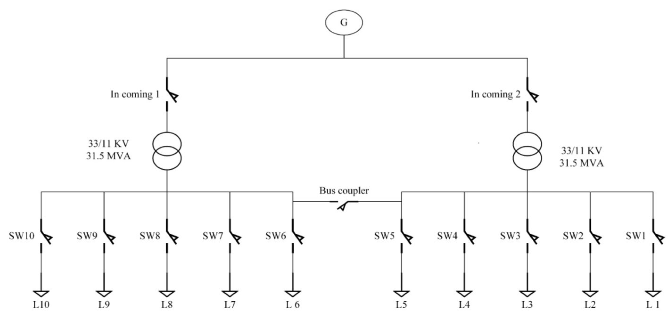
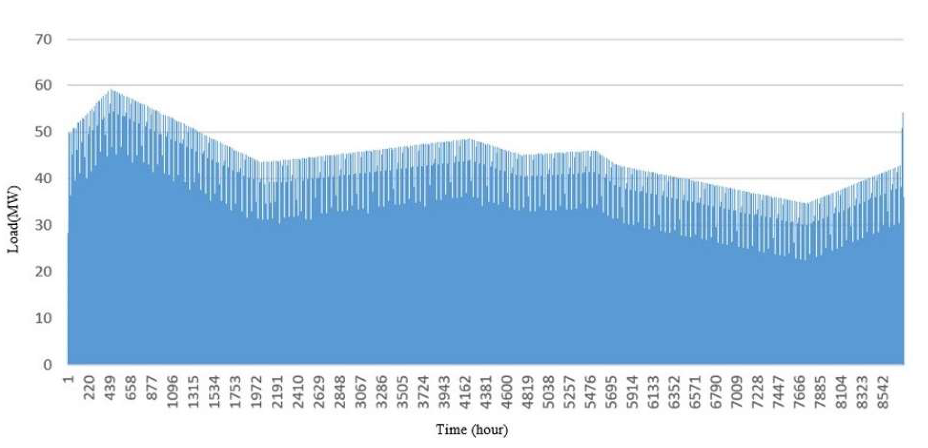
2.2. Collection of Input Data

The electrical load data at Iraq’s Al-Hussein Substation was obtained from the National Operation and Control Center for the city of Ramadi. Ten electrical feeders make up the station. The station provides service to a variety of clients, including residential customers, governmental organizations, industrial feeders, and commercial feeders, as shown in Figure 1. The substation is divided as follows:
  • Loads 1, 2, 3, 7 and 8 are residential feeders;
  • Loads 4 and 6 are the government institutions feeder;
  • Loads 5 and 9 are industrial feeders;
  • Load 10 is the commercial feeder.
The data is represented for years 2018, 2019, and 2020. Additionally, the data was listed based on hours (24 readings per day). It represents the maximum hourly electrical load data in MW. Additionally, 8760 readings are taken annually. Weather data included temperature °C and humidity %. NASA’s prediction of worldwide energy resources data set was used to obtain weather data. The date, hour, day, and month were used to organize the date’s data. For example, the fluctuation of the hourly consumption for the year 2020, which was used for training and testing, is shown in Figure 2. It demonstrates the historical trend in electricity consumption. When compared to other seasons, the value of consumption is higher in the winter. Figure 2 shows the importance of time factor information and contains crucial details about the load profile. So, it is assumed that it can be useful for predicting consumption.
The trend of the hourly temperature in °C for the year 2020 over time is illustrated in Figure 3. We also see that the temperature curve rises in the summer and falls in the winter. This also has an impact on the electrical load and forecasting processes. Additionally, the results will be shown later.
The hourly humidity trend in percentage for the year 2020 over time is shown in Figure 4. The inverse trend between the humidity factor and the temperature factor is seen. The pattern of these factors is similar to the rest of the other years. Therefore, we will investigate the link between these parameters shown in Figure 2, Figure 3 and Figure 4 and how it affects the predicted electrical load.

3. Methods of Load Forecasting

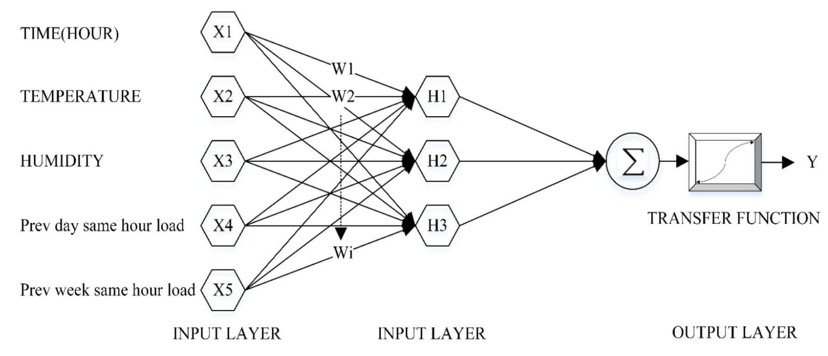
3.1. Artificial Neural Network (ANN)

An ANN is a computer system and mathematical tool that mimics the neural impulses and thought processes of the human brain via the use of interconnected structures or networks [28]. The basic processing units in artificial neural networks are called neurons. These cells are trained to perform in a manner like brain neurons by processing inputs and other factors [25]. An a rtificial neuron model that has been proposed is shown schematically in Figure 5.
X is the input, W is the weight, and Y is the output. H is the hidden layer. The ANN model consists of nodes that are interconnected and organized into layers [29]. Each node acts as a processing unit, as seen in Figure 5. Additionally, each of these nodes and layers works to address a specific problem. A total of three layers connects the neurons with nodes and weights. Neurons are made up of three parts; transfer functions, summation functions related to the contract, and weights attached to the contract. In addition, there are three layers in the neural network: the input, hidden, and output layers [3]. The private data is input and transmitted through the input layer using back-propagation until it reaches the output layer, where the weights are adjusted after each iteration to obtain the best mapping between the input and the output [30]. Three more inputs are almost always utilized in ANN programs:
  • Future-related entries;
  • Historical input that includes the max usual loads during a particular prior time;
  • Compressible input.
Feature selection is generally considered crucial for improving the performance of ANN algorithms during the training process for tasks such as load forecasting. In this study, we have taken the load value in MW for a specific hour and compared it with the load values for the same hour of the previous day and week. These values were used as inputs for the algorithm to determine the changes in load demand, including the amount and percentage of change. This information is used to identify whether the load demand is increasing or decreasing, which is crucial for load forecasting, as shown in Figure 5.
Neurons are the basic computational elements in artificial neural networks. These cells might deal with non-linear, non-parametric techniques that consider many different variables. Moreover the ANN models have capability to deal with nonlinear problems by using nonlinear activation function [31]. The flowchart for artificial neural network (ANNs) is shown in Figure 6. Changing the junction weights of the network to achieve the desired purpose is the task of the learning algorithm, which is the procedure used to train the network.
A transfer function is used to limit the amplitude of a neuron’s output. The following Equation (1) used in the transfer function to update every weight at each iteration:
W j i n e w = W j i o l d + ƞ   E W j i
where ( W j i ) and (ƞ) are the weights of the neurons and the learning rate, respectively. E represents the amount of error that can be calculated using Equation (2) as shown below:
E = k = 1 L j = 1 q b k j z k j 2
where ( b k j ) and ( z k j ) are the observed and predicted values by the ANN [32]. The use of linear and nonlinear transfer functions in artificial neural networks enables the application of solutions to complex and wide-ranging problems. Data is fed through the network in the feed-forward process. Additionally, errors are propagated through the network in the back-propagation process [33].

3.2. Adaptive Neuro-Fuzzy Inference System (ANFIS)

The combined ANFIS system includes fuzzy logic FL and artificial neural networks ANN. It is also a method that can be applied in artificial intelligence AI systems to predict electric loads. ANFIS is a hybrid system that combines learning in the ANN style with human logic in the FL style [34]. It is adaptable to networks where certain nodes are linked by directed links. Each node represents a processing element in addition to the linkages that join the nodes. Some nodes in ANFIS can be adjusted, while others are fixed. The adaptive nodes only have a single output. The adaptable nodes depend on a few variables that can be modified, such as the local weather conditions. The rule for updating these parameters, which is to minimize a prescribed error that measures the difference between the actual load (output) and expected output, is one of the most crucial things to understand. The ANFIS seen in Figure 7 is composed of 5 layers. Adaptive layers are represented by squares, whereas non-adaptive layers are represented by circles.
As indicated in Figure 7, we look at the prediction of the electrical load using adaptation. The fuzzy inference system is taken into consideration and has two inputs, X and Y, and one output, P. We take that into account while modeling IF-AND-THEN rules using a first-order Sugeno fuzzy model and formulated in Equations (3) and (4) [23]:
Rule   1 :   IF   X   is   A 1   AND   Y   is   B 1   THEN   P 1 = Ƥ 1 X + ɋ 1 Y + r 1
Rule   2 :   IF   X   is   A 2   AND   Y   is   B 2   THEN   P 2 = Ƥ 2 X + ɋ 2 Y + r 2
where A1, A2, B1, and B2 are the input membership functions. The neuron’s set parameters are Ƥ i , ɋ i , and r i , which are represented in Equations (5)–(7):
Ƥ 1 = W i ¯   ×   X 1
ɋ 1 = W i ¯   ×   X 2
r 1 = W i ¯
Additionally, W1 and W2 are the firing strength regulations as in Equations (8) and (9):
W 1 = µ A 1   ×   µ A B 1
W 2 = µ A 2   ×   µ A B 2
where µ is the membership degree. W1 and W2 are expressed in Equation (10) as follows:
P = W 1 Ƥ 1 + W 2 Ƥ 2 W 1 + W 1 = W 1 P 1 ¯ + W 2 P 2 ¯
ANFIS employs a hybrid learning algorithm that combines the error back-propagation EBP and least-squares estimator LSE techniques. EBP is performed in the first layer of the ANFIS structure [6], whereas LSE is performed in the fourth layer. The parameter from the fuzzy membership function that is non-linear toward system output is employed in the first layer. Many different membership function types, including, Gaussian, triangular, and trapezoidal, have been tested and trained in the ANFIS system. In this work, we selected the type of (triangular), which is defined in Equation (11):
f   ( x ,   a ,   b ,   c ) = 0 c x a x a b a a x b c x c b b x c
where x is the input data, a represents the standard deviation, b the slopes must always be positive, and c represents the mean.
For the present stage, an ANFIS input is supplied. These inputs are fuzzified with membership functions and trained using training data measured under normal and abnormal conditions to obtain the best membership function parameters. The ANFIS training and testing flowchart is shown in Figure 8.

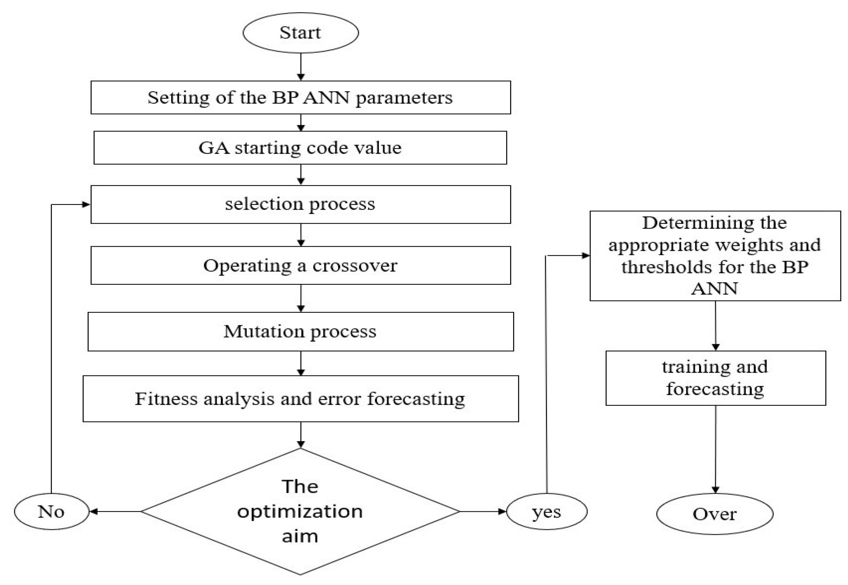
3.3. Schematic of ANN Optimized by GA

A technique called a genetic algorithm GA is based on a natural selection process that mimics biological evolution and can be used to solve both unnatural and constrained optimization problems. It mixes functional optimizations with the adaptable properties of natural genetics or the methods of organ natural selection. The ideal solution is found through randomizer information exchange by simulating the ability to survive among string structures. Every time there is a reproduction, a new batch of synthetic strings is created from the remains of the oldest, fittest individuals. It effectively uses historical data to make assumptions about a new search point with better performance predicted [35].
The genetic algorithm is effective at delivering the best results by considering more data and potentially offering larger search spaces. A GA that creates a population of n chromosomes is suitable for the situation at work. Each population’s chromosome x’s fitness f(x) is determined as well. Progress after each step is continuously made until the new population is finished. The parents are crossed over to create new offspring using a crossover prospect. In the absence of crossover, the offspring will be an identical copy of the parents. Additionally, new mutations are created at each locus with the aid of mutation probability. Afterward, after adding fresh offspring to the newly created population, a custom new population was built for the algorithm’s additional summation. If the last requirement is met, stop, then switch back to the current population that is most suitable. Thereafter, to retain fitness, the algorithm will automatically finish when the population converges on the effective solutions [36].
When GA and ANN are combined, the initial neurons in the BP artificial neural network model’s weights and thresholds are randomly selected, which could result in local minima. The BP artificial neural network, which combines ANN structure determination, GA optimization, and ANN prediction, is optimized using genetic algorithms GA. Figure 9 lists the GA processes for determining the ideal weight and threshold.

3.4. Error Validation

The user may confirm the trained algorithm can generate low-error forecasts After testing [18], the proposed algorithm forecast plot was compared to the test set data plot. The mean absolute percentage error MAPE and root mean square error RMSE were determined to decrease the forecast error. In this work, the error was validated by two Equations (12) and (13):
RMSE = 1 n i = 1 n ( y i y i ) 2
MAPE = 1 n 1 n ( y i y i ) y i   ×   100
Here, n is the number of samples, y i is the predicted value of the model, and y i is the actual desired value.

4. Methodology

4.1. Utilizing MATLAB to Implement the ANN’s Input Data

At first, we used weather data and statistics on the electrical load in Iraq from Al Hussein station for a year (from 1 January 2018 to 31 December 2018). The time data is divided into date, hour, day, and month. The weather data includes temperature in °C and humidity in %. The distribution of the data takes place in hours, meaning that it is given per hour of the day for all data. The duration was 365 days. Thus, each column in the provided data is 24 × 365 = 8760 characters long. Additionally, there are 7 columns in all. Thus, there are 61,320 cells in the entire Excel file. All data including weather and load data were entered into MATLAB to record the time of day for each input. 8760 rows of columns are imported from the Excel sheet. Each column has been given a specific variable to describe its impact on the load forecasting process. The entire data set was divided into two groups, the training set and the test set divided as:
  • 80% training—20% testing;
  • 70% training—30% testing;
  • 60% training—40% testing;
  • 50% training—50% testing.
The following inputs were used to create the training set:
  • Time in (hours);
  • Temperature (°C);
  • Humidity (%);
  • Previous Day Same Hour Load (MW);
  • Previous Week Same Day Same Hour Load (MW).
The number of neurons in ANN hidden layers was defined as 5, 10, and 15. The backpropagation training of the feed-forward ANN was performed using the training function of the Levenberg–Marquardt algorithm when using the training predictor dataset and a target dataset. This procedure iteratively changed the internal weight and bias parameters of the ANN to provide an output with a low error rate. The target dataset consists of the actual load values for a given predictor dataset by using only the training predictor dataset. The ANN was evaluated after training using the sample data provided in this stage. The forecast results were saved and the entire ANN training and testing with forecasting procedure was repeated a predetermined number of times. The results in Table 1 showed the algorithm function (Levenberg–Marquardt) for the year 2018. Additionally, it showed that increasing the number of hidden layers and the test ratio relative to the training ratio leads to an increased error rate in both MAPE and RMSE values. The best result appeared at a splitting rate of 80% training and 20% testing and when the number of hidden layers was 5. This yielded 3.2451% for the MAPE and 0.4248 for the RMSE, which are acceptable values. The error values correspond to days where a scheduled or unexpected outage or another sudden load shift occurred in the real load profile. The numbers used for the minimal inputs and the number of hidden-layer neurons directly affected the length of ANN training in the MATLAB software.
The same procedure appears in the year 2019. The best result appeared at a splitting rate of 80% training and 20% testing, and when the number of hidden layers was 5 with 3.7452% for the MAPE and 0.3177 for the RMSE as shown in Table 2. The year 2020 will be adopted as a source for matching and comparison.
The forecasted electrical load for the years 2018 and 2019 were plotted against time on a graph, and the forecasted load with test data (the actual load) was compared. A part of this graph is shown in Figure 10 and Figure 11. The forecasted electrical load compared to the actual load has a slight variance, as seen in the graph, where the solid red line represents the actual electrical load, and the blue dashed line represents the forecasted electrical load.
The regression value of the test set of the year 2018 was R = 0.99416, while the regression value of the training set was R = 0.99324. For validation, R = 0.99468, and R = 0.9936 for all, which are also acceptable. Additional, similar, and close values for 2019 are shown in Figure 12.

4.2. Implementation of the Adaptive Neuro-Fuzzy Inference System ANFIS Using MATLAB

The ANFIS modeling standard is modified to properly implement the membership function and to minimize output error and maximize performance indication. The data is used for training, testing, and verification. The next stage is to construct a fuzzy inference system FIS and choose a type of membership function. Table 3 and Table 4 display the tested and trained triangular membership function. Now, we have the required inputs, which are time, temperature, humidity, and previous load values for the years 2018 and 2019, from the same Excel table that was used previously in the ANN technique with the same division, i.e., 8760 h for all data. To be used with the input of the membership function, it produces rules in this way by listing all possible installations of the membership function for all inputs. When the algorithm is called in ANFIS, we perform looping for the electrical load values for the year to be worked on. In other words, during the test, the electrical load’s last value returns to become the first value. Additionally, the test is replicated by reading the loads repeatedly to determine the values and percentages of change while running tests with other variables [19]. Furthermore, the proposed ANFIS was defined to have the following number of membership functions: 3, 4, and 5. Epoch refers to a complete pass through the entire training dataset during the training process of a machine learning model. The study experimented with different epoch counts of 20, 30, and 40, where each epoch count indicates the number of times all the training data is used to update the model once. By varying the epoch count, this study aims to analyze the impact of the number of iterations on the performance of the model and determine the optimal epoch count for the given dataset. When we decided to change the membership function type while running tests and training, triangular membership functions were chosen because changing the form of a membership function has little to no impact on the extracted data or has a small impact that is not noticeable. Moreover, it has a small impact on the numbers of epochs, where the effect was very small. Only the number of membership functions affected the MAPE value’s outcome, which is also a rather small variation. So, based on the 5-membership function with 40 epoch numbers, we have low error rates of 2.8532% for the MAPE and 0.3301 for the RMSE in 2018, which are acceptable, as shown in Table 3. Additionally, we obtained 2.8036% for the MAPE and 0.3125 for the RMSE in 2019, as shown in Table 4. The year 2020 will be adopted as a source for matching and comparison.
To compare the actual load to the predicted load for the years 2018 and 2019, the actual load was plotted against the hourly time. Figure 13 and Figure 14, which are displayed below, show a part of this graph. The forecasted plot from the test data load has a slight variance against the real load; the previous real electrical load values are represented by the red continuous line, while the predicted electrical load values are represented by the dashed blue line.

4.3. Genetic Algorithms (GA) Optimize ANN Predictions

Genetic algorithm (GA) is used to optimize the BP artificial neural network’s predictions. The weights and thresholds between the initial neurons of the BP artificial neural network model are selected randomly. Based on the ANN outputs that have the lowest error rate, which are in 5 hidden layers and 80% training and 20% testing, the data will be normalized and entered into GA for processing. The GA was shown to include hidden layers of 5, 10, and 15. For the year 2018, the best result appeared when the number of hidden layers was 5, with 1.8663% for the MAPE and 0.0476% for the RMSE, as shown in Table 5. For the year 2019, the best result appeared when the number of hidden layers was 5, with 2.4571% for the MAPE and 0.0476 for the RMSE, as shown in Table 6. The year 2020 will be adopted as a source for matching and comparison.
To compare the actual load to the predicted load for the years 2018 and 2019. The actual load was plotted against the hourly time. Figure 15 and Figure 16, which are displayed below, show a part of this graph. The predicted plot from the test data load has a slight variance against the real load; the previous real electrical load values are represented by the red continuous line, while the predicted electrical load values are represented by the dashed blue line.

4.4. Results of Tests and Training in Purposed Techniques

This study described and focused on long-term load forecasting, which involves the use of a large amount of data. In order to make predictions, we used a maximum value approach for each month of the year, as detailed in Table 7.
We employ ANN–GA (Artificial Neural Networks–Genetic Algorithm) to establish a relationship of the predicted load between relative humidity and temperatures. During the forecasting process in 2018, we obtained electrical load values for the year 2019. The predicted values for 2018, as determined by ANN, ANFIS, and ANN–GA, were compared to the actual values (target) for 2019. The results indicate that ANN–GA produced more accurate predictions than the other two methods.
We repeated this process for the year 2019, comparing the predicted electrical load values for that year to the actual values (target) for 2020. Once again, the convergence between ANN–GA and the actual values was superior to the other methods. Addition-ally, the percentage error rates between these algorithms for the years 2018 and 2019 confirmed the superiority of ANN–GA over the other methods.

5. Conclusions and Suggestions

In this study, we utilized a sample of annual data in hours and applied three significant algorithms instead of using short-term patterns or dividing the data into days, weeks, months, holidays, etc., and including them in different algorithms for forecasting. By using the ANN, ANFIS, and ANN–GA techniques, the performance of all methods was evaluated for electrical load forecasting and demonstrated their dynamic response to the weather variables used in this study.
The results showed that ANN–GA performed better than the other two methods (ANN and ANFIS) in terms of accuracy and error rate for long-term load forecasting, with 1.866% for the MAPE and 0.047 for the RMSE for the year 2018. Compared to ANFIS technology with 2.853% for the MAPE and 0.330 for the RMSE and ANN with 3.245% for the MAPE and 0.424 for the RMSE in all test and training ratios.
At 2.457% for the MAPE and 0.062 for the RMSE for the year 2019, ANN–GA also reported good accuracy and error rate results compared to ANN technology, which had 5.017% for the MAPE and 0.654 for the RMSE in all test and training ratios, and ANFIS technology, which had 2.807% and 0.312 for the MAPE and RMSE, respectively.
Additionally, this study found that increasing the number of hidden layers and testing and training ratios in ANN leads to a decrease in accuracy and an increase in error rate. On the other hand, ANFIS technology shows a small increase in the error rate due to the effect of the membership function, which is hardly noticeable. The same applies to ANN–GA in terms of implementation time. Overall, this study suggests that ANN–GA is a more accurate and efficient method for long-term load forecasting compared to ANN and ANFIS.
Although the results of ANFIS appeared to be good in terms of convergence of the predicted values with the actual values of the electrical loads compared with ANN, the ANN technique is the most receptive and adaptive to all kinds of linear and non-linear parameters and inputs, such as time, weather, economic factors, etc., compared with the ANFIS technique, which is limited in the types of parameters that can be trained and tested and is difficult to implement. As it uses the input values of ANN to work on and enhance them, ANN–GA naturally assumes the same characteristics as ANN in this field. The reason ANN–GA technology is superior to other approaches is that it normalizes the data and ANN outputs that have been forecasted before determining the optimal fitness values, reformatting them, and using them. This is one of the features of hybrid systems, which includes other hidden layers to achieve the best optimal values. They choose the parameters’ best values, and thus they have the lowest error rate.
In addition to weather variables, there are other factors and variables that can significantly affect electric load forecasts. For example, economic factors, such as electricity prices and the total number of customers on a specific electrical network, can also be included in forecasting models to improve their reliability. Further research can explore the impact of these variables on electric load forecasting and develop models that integrate them effectively. By incorporating more factors and variables, we can improve the accuracy and robustness of electric load forecasting and make better decisions regarding energy planning and management.

Author Contributions

Conceptualization, A.M.M.A.-Q., A.B. and Y.A.; literature studies, A.M.M.A.-Q., A.B. and Y.A.; research methodology, A.M.M.A.-Q.; research and data analysis, A.M.M.A.-Q., A.B. and Y.A.; writing—original draft preparation, A.M.M.A.-Q., A.B. and Y.A.; writing—review and editing, A.M.M.A.-Q., A.B. and Y.A. All authors have read and agreed to the published version of the manuscript.

Funding

This research received no external funding.

Data Availability Statement

Not applicable.

Acknowledgments

This research was conducted as part of the Master’s thesis titled “Load forecasting models for power distribution systems”, which is being carried out under the auspices of the Yildiz Technical University Institute of Science.

Conflicts of Interest

The authors declare no conflict of interest.

References

  1. Matijaš, M. Electric Load Forecasting Using Multivariate Meta-Learning. Ph.D. Thesis, Fakultet elektrotehnike i računarstva, Sveučilište u Zagrebu, Zagreb, Croatia, 2013. [Google Scholar]
  2. Kotriwala, A.M. Load Forecasting for Temporary Power Installations. Master’s Thesis, KTH Royal Institute of Technology, Stockholm, Sweden, 2017. [Google Scholar]
  3. Han, L.; Peng, Y.; Li, Y.; Yong, B.; Zhou, Q.; Shu, L. Enhanced Deep Networks for Short-Term and Medium-Term Load Forecasting. IEEE Access 2018, 7, 4045–4055. [Google Scholar] [CrossRef]
  4. Nti, I.K.; Teimeh, M.; Nyarko-Boateng, O.; Adekoya, A.F. Electricity load forecasting: A systematic review. J. Electr. Syst. Inf. Technol. 2020, 7, 13. [Google Scholar] [CrossRef]
  5. Arfoa, A.A. Long-term load forecasting of southern governorates of Jordan distribution electric system. Energy Power Eng. 2015, 7, 242. [Google Scholar] [CrossRef] [Green Version]
  6. Shareef, H.; Ahmed, M.; Mohamed, A.; Al Hassan, E. Review on home energy management system considering demand responses, smart technologies, and intelligent controllers. IEEE Access 2018, 6, 24498–24509. [Google Scholar] [CrossRef]
  7. Al Mamun, A.; Sohel, M.; Mohammad, N.; Sunny, M.; Dipta, D.; Hossain, E. A comprehensive review of the load forecasting techniques using single and hybrid predictive models. IEEE Access 2020, 8, 134911–134939. [Google Scholar] [CrossRef]
  8. Baek, S.-M. Mid-term load pattern forecasting with recurrent artificial neural network. IEEE Access 2019, 7, 172830–172838. [Google Scholar] [CrossRef]
  9. Ibraheem, I.K.; Ali, M.O. Short term electric load forecasting based on artificial neural networks for weekends of Baghdad power grid. Int. J. Comput. Appl. 2014, 89, 30–37. [Google Scholar]
  10. Abdullah, A.G.; Suranegara, G.; Hakim, D.L. Hybrid PSO-ANN application for improved accuracy of short term load forecasting. WSEAS Trans. Power Syst. 2014, 9, 51. [Google Scholar]
  11. Alawode, K.O.; Oyedeji, M.O. Comparison of Neural Network models for Load Forecasting in Nigeria Power Systems. Int. J. Renew. Energy Technol. 2013, 2, 218–222. [Google Scholar]
  12. Ali, D.; Yohanna, M.; Ijasini, P.; Garkida, M.B. Application of fuzzy–Neuro to model weather parameter variability impacts on electrical load based on long-term forecasting. Alex. Eng. J. 2018, 57, 223–233. [Google Scholar] [CrossRef]
  13. Ammar, N.; Sulaiman, M.; Nor, A.F.M. Long-term load forecasting of power systems using artificial neural network and ANFIS. ARPN J. Eng. Appl. Sci. 2018, 13, 828–834. [Google Scholar]
  14. Xu, Y.; Cai, J.; Milanović, J.V. On accuracy of demand forecasting and its extension to demand composition forecasting using artificial intelligence based methods. In Proceedings of the IEEE PES Innovative Smart Grid Technologies, Europe, Istanbul, Turkey, 12–15 October 2014; pp. 1–6. [Google Scholar]
  15. Panda, S.K.; Mohanty, S.; Jagadev, A.K. Long term electrical load forecasting: An empirical study across techniques and domains. Indian J. Sci. Technol. 2017, 10, 1–16. [Google Scholar] [CrossRef]
  16. GÖKGÖZ, F.; Filiz, F. Electricity load forecasting via ANN approach in Turkish electricity markets. Bilgi Yönetimi 2020, 3, 170–184. [Google Scholar] [CrossRef]
  17. Arvanitidis, A.I.; Bargiotas, D.; Daskalopulu, A.; Laitsos, V.; Tsoukalas, L.H. Enhanced Short-Term Load Forecasting Using Artificial Neural Networks. Energies 2021, 14, 7788. [Google Scholar] [CrossRef]
  18. Pham, M.-H.; Nguyen, M.-N.; Wu, Y.-K. A novel short-term load forecasting method by combining the deep learning with singular spectrum analysis. IEEE Access 2021, 9, 73736–73746. [Google Scholar] [CrossRef]
  19. Oprea, S.-V.; Bâra, A. Machine learning algorithms for short-term load forecast in residential buildings using smart meters, sensors and big data solutions. IEEE Access 2019, 7, 177874–177889. [Google Scholar] [CrossRef]
  20. Selvi, M.V.; Mishra, S. Investigation of performance of electric load power forecasting in multiple time horizons with new architecture realized in multivariate linear regression and feed-forward neural network techniques. IEEE Trans. Ind. Appl. 2020, 56, 5603–5612. [Google Scholar] [CrossRef]
  21. Nespoli, A.; Leva, S.; Mussetta, M.; Ogliari, E.G.C. A Selective Ensemble Approach for Accuracy Improvement and Computational Load Reduction in ANN-Based PV Power Forecasting. IEEE Access 2022, 10, 32900–32911. [Google Scholar] [CrossRef]
  22. ZulfiqAr, M.; Kamran, M.; Rasheed, M.B.; Alquthami, T.; Milyani, A.H. A Short-Term Load Forecasting Model Based on Self-Adaptive Momentum Factor and Wavelet Neural Network in Smart Grid. IEEE Access 2022, 10, 77587–77602. [Google Scholar] [CrossRef]
  23. Faraji, J.; Ketabi, A.; Hashemi-Dezaki, H.; Shafie-Khah, M.; Catalão, J.P. Optimal day-ahead self-scheduling and operation of prosumer microgrids using hybrid machine learning-based weather and load forecasting. IEEE Access 2020, 8, 157284–157305. [Google Scholar] [CrossRef]
  24. Rafi, S.H.; Deeba, S.R.; Hossain, E. A short-term load forecasting method using integrated CNN and LSTM network. IEEE Access 2021, 9, 32436–32448. [Google Scholar] [CrossRef]
  25. Mahmud, K.; Ravishankar, J.; Hossain, M.J.; Dong, Z.Y. The impact of prediction errors in the domestic peak power demand management. IEEE Trans. Ind. Inform. 2019, 16, 4567–4579. [Google Scholar] [CrossRef]
  26. Mansoor, H.; Rauf, H.; Mubashar, M.; Khalid, M.; Arshad, N. Past vector similarity for short term electrical load forecasting at the individual household level. IEEE Access 2021, 9, 42771–42785. [Google Scholar] [CrossRef]
  27. Haq, M.R.; Ni, Z. A new hybrid model for short-term electricity load forecasting. IEEE Access 2019, 7, 125413–125423. [Google Scholar] [CrossRef]
  28. Song, J.; Xue, G.; Pan, X.; Ma, Y.; Li, H. Hourly heat load prediction model based on temporal convolutional neural network. IEEE Access 2020, 8, 16726–16741. [Google Scholar] [CrossRef]
  29. Chen, K.; Chen, K.; Wang, Q.; He, Z.; Hu, J.; He, J. Short-term load forecasting with deep residual networks. IEEE Trans. Smart Grid 2018, 10, 3943–3952. [Google Scholar] [CrossRef] [Green Version]
  30. Kong, W.; Dong, Z.Y.; Jia, Y.; Hill, D.J.; Xu, Y.; Zhang, Y. Short-term residential load forecasting based on LSTM recurrent neural network. IEEE Trans. Smart Grid 2017, 10, 841–851. [Google Scholar] [CrossRef]
  31. Dattatrey, M.; Tiwari, A.K.; Ghoshal, B.; Singh, J. Predicting bone modeling parameters in response to mechanical loading. IEEE Access 2019, 7, 122561–122572. [Google Scholar] [CrossRef]
  32. Akarslan, E.; Hocaoglu, F.O. Electricity demand forecasting of a micro grid using ANN. In Proceedings of the 2018 9th International Renewable Energy Congress (IREC), Hammamet, Tunisia, 20–22 March 2018; pp. 1–5. [Google Scholar]
  33. Liu, H.; Wang, Y.; Wei, C.; Li, J.; Lin, Y. Two-stage short-term load forecasting for power transformers under different substation operating conditions. IEEE Access 2019, 7, 161424–161436. [Google Scholar] [CrossRef]
  34. Moradzadeh, A.; Mohammadi-Ivatloo, B.; Abapour, M.; Anvari-Moghaddam, A.; Roy, S.S. Heating and cooling loads forecasting for residential buildings based on hybrid machine learning applications: A comprehensive review and comparative analysis. IEEE Access 2021, 10, 2196–2215. [Google Scholar] [CrossRef]
  35. Lin, T.; Pan, Y.; Xue, G.; Song, J.; Qi, C. A novel hybrid spatial-temporal attention-LSTM model for heat load prediction. IEEE Access 2020, 8, 159182–159195. [Google Scholar] [CrossRef]
  36. Ouyang, T.; He, Y.; Li, H.; Sun, Z.; Baek, S. Modeling and forecasting short-term power load with copula model and deep belief network. IEEE Trans. Emerg. Top. Comput. Intell. 2019, 3, 127–136. [Google Scholar] [CrossRef] [Green Version]
Figure 1. Al-Hussein Distribution 33/11.5 kV 31.5 MVA Substation.
Energies 16 02919 g001
Figure 2. The fluctuation of the Al-Hussein substation’s hourly load in 2020.
Energies 16 02919 g002
Figure 3. The city of Ramadi’s temperature variance in 2020.
Energies 16 02919 g003
Figure 4. The city of Ramadi’s humidity variance in 2020.
Energies 16 02919 g004
Figure 5. A schematic representation of a suggested ANN model.
Energies 16 02919 g005
Figure 6. Flowchart of artificial neural network (ANN).
Energies 16 02919 g006
Figure 7. The ANFIS architecture.
Energies 16 02919 g007
Figure 8. Flowchart of ANFIS training and testing process.
Energies 16 02919 g008
Figure 9. Flowchart of the ANN with GA optimization.
Energies 16 02919 g009
Figure 10. Actual and forecasted load for the purposed ANN for the year 2018.
Energies 16 02919 g010
Figure 11. Actual and forecasted load ANN in 2019.
Energies 16 02919 g011
Figure 12. The Purposed (ANN) 2018 Actual and Forecasted Load (regression Plot).
Energies 16 02919 g012
Figure 13. Actual and forecasted load for the purposed ANFIS for the year 2018.
Energies 16 02919 g013
Figure 14. Actual and forecasted load ANFIS in 2019.
Energies 16 02919 g014
Figure 15. Actual and forecasted load for the purposed ANN–GA for the year 2018.
Energies 16 02919 g015
Figure 16. Actual and forecasted load for the purposed ANN–GA for the year 2019.
Energies 16 02919 g016
Table 1. Training and testing results for the purposed ANN for the year 2018.
Splitting Rate80% Training—20% Testing70% Training—30% Testing60% Training—40% Testing50% Training—50% Testing
Training FunctionsLevenberg–MarquardtLevenberg–MarquardtLevenberg–MarquardtLevenberg–Marquardt
5 hidden layersMAPE%3.2451MAPE%5.3756MAPE%5.4447MAPE%5.9299
RMSE0.4248RMSE0.6928RMSE0.7059RMSE0.7318
10 hidden layersMAPE%5.4319MAPE%7.5222MAPE%7.6136MAPE%7.9921
RMSE0.7206RMSE1.0655RMSE1.1513RMSE1.2919
15 hidden layersMAPE%6.3252MAPE%8.2533MAPE%8.5213MAPE%9.3836
RMSE0.8350RMSE1.0885RMSE1.2918RMSE1.3370
Table 2. Training and test results for the purposed ANN for the year 2019.
Splitting Rate80% Training—20% Testing70% Training—30% Testing60% Training—40% Testing50% Training—50% Testing
Training FunctionsLevenberg–MarquardtLevenberg–MarquardtLevenberg–MarquardtLevenberg–Marquardt
5 hidden layersMAPE%3.7452MAPE%6.2402MAPE%6.5315MAPE%6.8512
RMSE0.3177RMSE0.8452RMSE0.8997RMSE0.9682
10 hidden layersMAPE%5.4613MAPE%8.1691MAPE%8.8338MAPE%9.2921
RMSE1.1954RMSE1.2181RMSE1.5890RMSE1.7019
15 hidden layersMAPE%6.9019MAPE%8.4002MAPE%9.1607MAPE%10.2756
RMSE1.2876RMSE1.3403RMSE1.6893RMSE1.7601
Table 3. Results for the purposed ANFIS for the year 2018.
Epoch Number 203040
Membership Function TypeTriangular Membership FunctionsTriangular Membership FunctionsTriangular Membership Functions
3 membership functionsMAPE%3.0165MAPE%3.0073MAPE%3.0039
RMSE0.3294RMSE0.3294RMSE0.3294
4 membership functionsMAPE%2.9318MAPE%2.9317MAPE%2.9330
RMSE0.3297RMSE0.3297RMSE0.3297
5 membership functionsMAPE%2.8785MAPE%2.8761MAPE%2.8532
RMSE0.3301RMSE0.3302RMSE0.3301
Table 4. Results for the purposed ANFIS for the year 2019.
Epoch Number 203040
Membership Function TypeTriangular Membership FunctionsTriangular Membership FunctionsTriangular Membership Functions
3 membership functionsMAPE%2.9065MAPE%2.9026MAPE%2.9005
RMSE0.3117RMSE0.3117RMSE0.3117
4 membership functionsMAPE%2.8273MAPE%2.8299MAPE%2.8303
RMSE0.3121RMSE0.3121RMSE0.3135
5 membership functionsMAPE%2.8189MAPE%2.8118MAPE%2.8036
RMSE0.3125RMSE0.3125RMSE0.3125
Table 5. Results for the Purposed ANN–GA for the year 2018.
Splitting RateError %
5 hidden layersMAPE%1.8663
RMSE0.0476
10 hidden layersMAPE%4.8722
RMSE0.1889
15 hidden layersMAPE%5.9395
RMSE0.1714
Table 6. Results for the Purposed ANN–GA for the year 2019.
Splitting RateError %
5 hidden layersMAPE%2.4571
RMSE0.0623
10 hidden layersMAPE%3.7701
RMSE0.0668
15 hidden layersMAPE%5.9110
RMSE0.1572
Table 7. Output results of the purposed techniques.
MonthLong-Term InputsTargetANNANFISANN–GA
Temp (°C)Hum (%)ACTUAL
2018 (MW)
ACTUAL
2019
(MW)
ACTUAL
2020
(MW)
Predicted
2018
(MW)
Predicted
2019 (MW)
Predicted
2018
(MW)
Predicted
2019 (MW)
Predicted
2018
(MW)
Predicted
2019
(MW)
JAN20.4097.4453.85655.8559.3553.8855.8456.4456.4354.2759.96
FEB23.4296.8151.01253.0156.5150.9652.9451.5352.9853.9754.45
MAR35.7383.1243.66545.6658.9243.6945.6744.8344.9146.2047.49
APR33.3795.6239.91541.9145.4739.7941.7841.2043.9440.1544.40
MAY39.8280.7541.62543.6247.1841.5043.4849.5844.0242.2644.41
JUN41.4261.4443.05045.0548.5542.9844.9643.8647.6745.4447.88
JULY42.5560.3142.15644.0047.3542.1643.9841.5544.3544.7045.46
AUG49.5960.2540.61542.6146.1140.5542.5442.8543.6342.7643.90
SEP42.8155.1937.17439.1742.5737.1139.0839.0140.1440.9540.87
OCT38.0086.6234.07436.0739.4734.0936.0638.1439.4034.7037.02
NOV26.2091.2031.37433.3737.0731.2333.2933.8635.5033.4136.86
DEC20.1397.6637.37439.454.1837.1639.2337.6340.0037.3440.16
MAPE3.245%5.017%2.853%2.807%1.866%2.457%
RMSE0.424%0.654%0.330%0.312%0.047%0.062%
Disclaimer/Publisher’s Note: The statements, opinions and data contained in all publications are solely those of the individual author(s) and contributor(s) and not of MDPI and/or the editor(s). MDPI and/or the editor(s) disclaim responsibility for any injury to people or property resulting from any ideas, methods, instructions or products referred to in the content.

