
EU: The Effect of Energy Factors on Economic Growth
Abstract
:1. Introduction
2. Materials and Methods
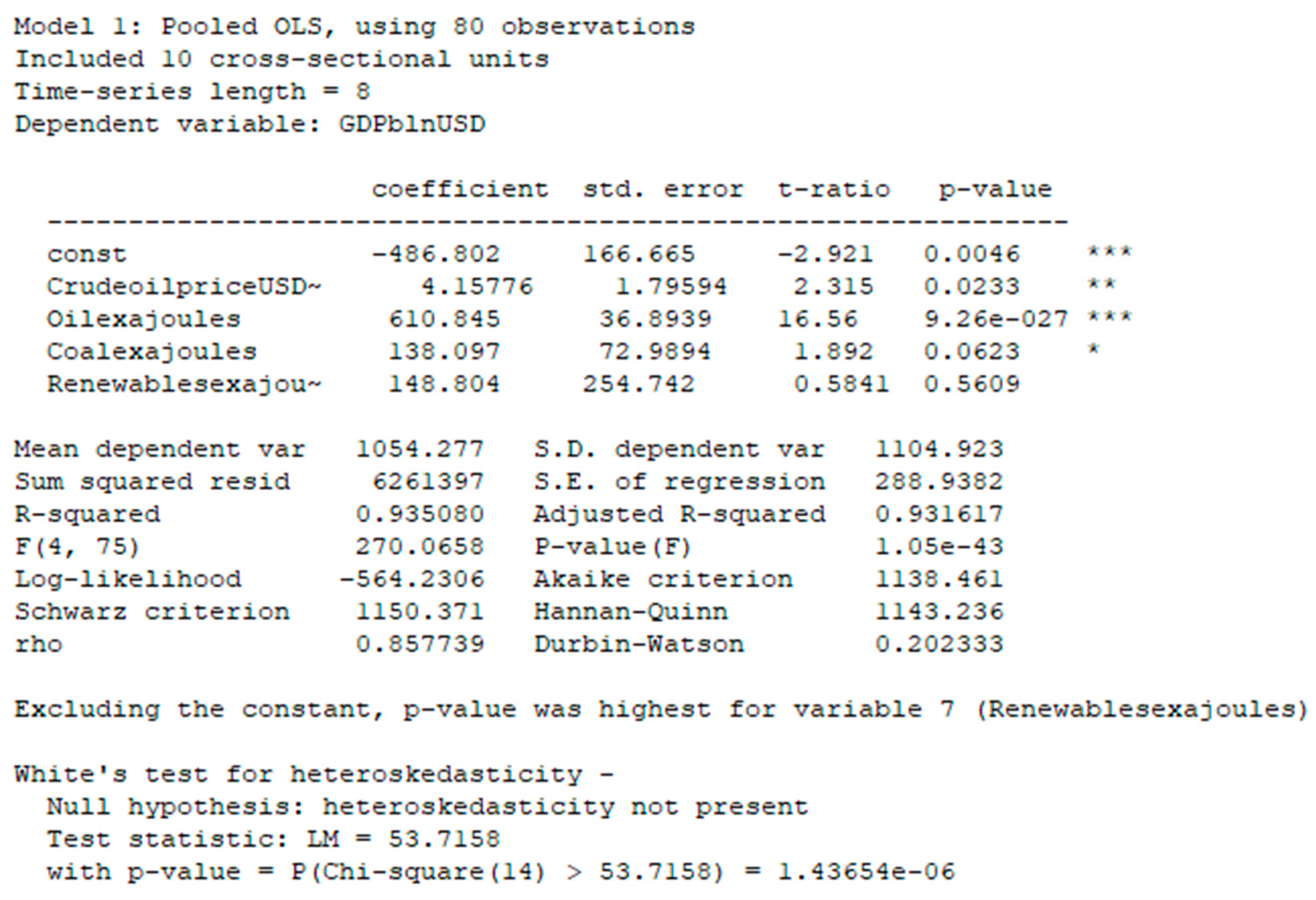
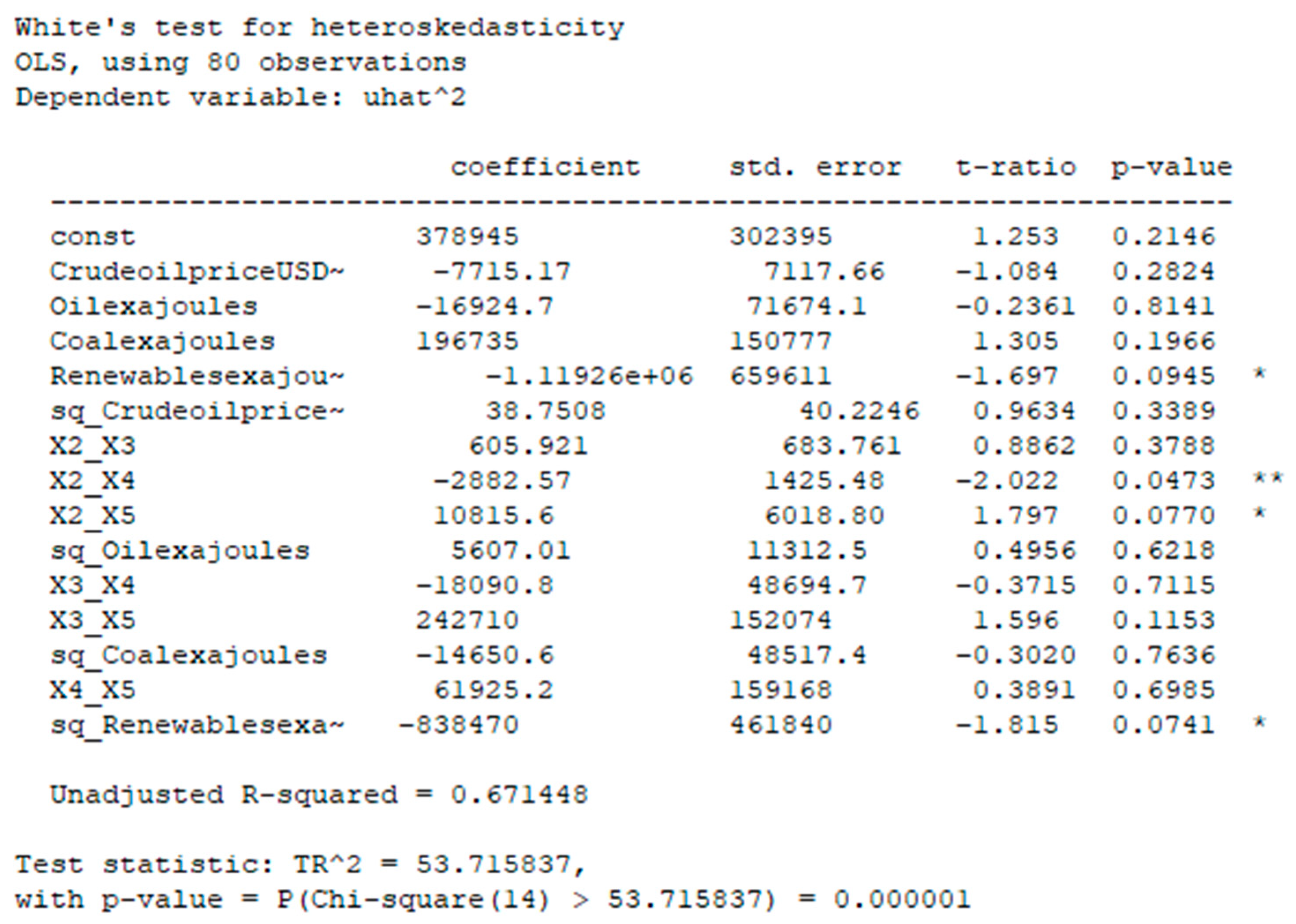
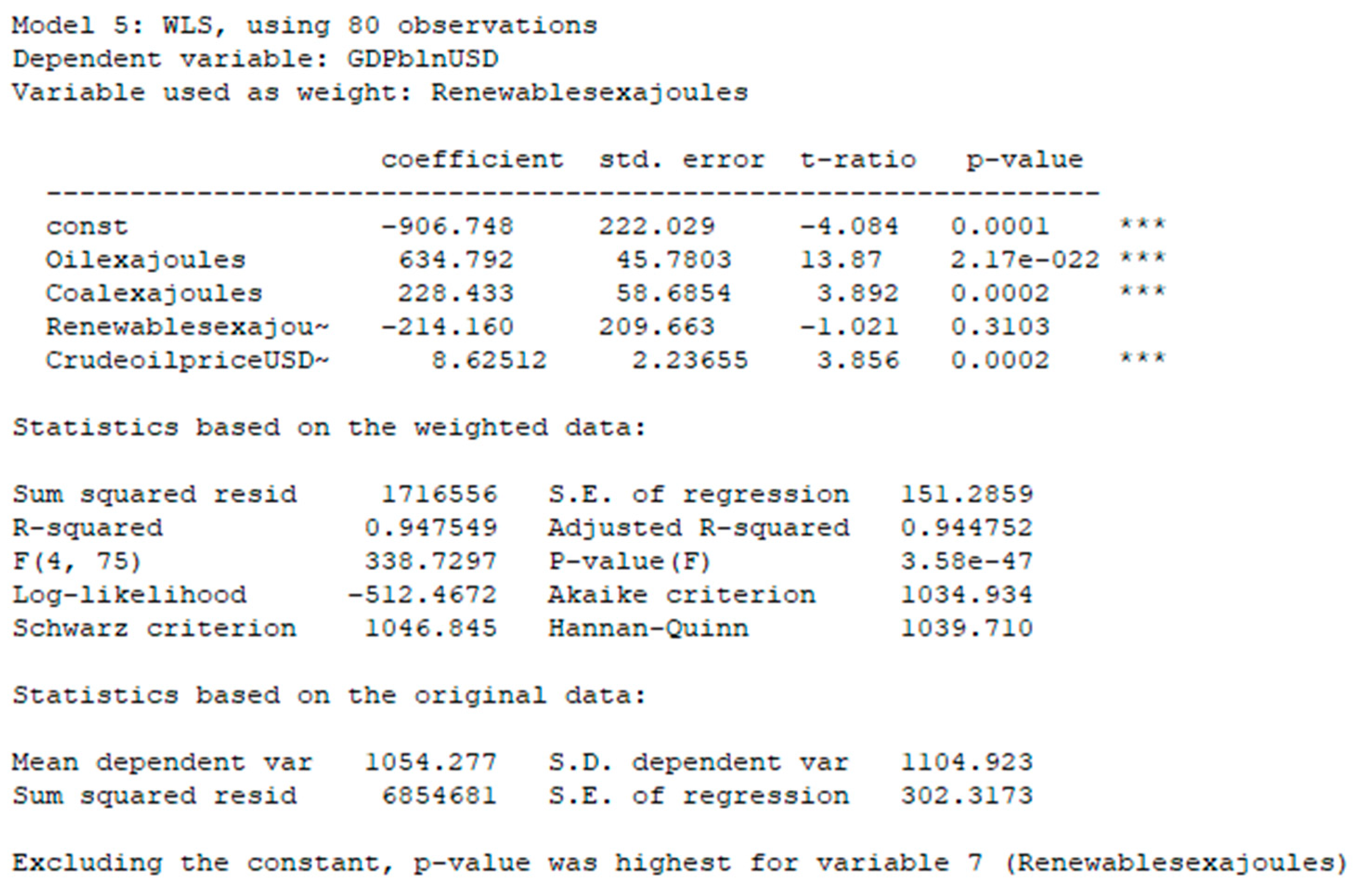
2.1. Building Models, Modelling, Testing Models
- Crude oil price per barrel.
- Crude oil consumption (exajouls).
- Coal consumption (exajouls).
- Renewable energy consumption (exajouls).
- Time dummy variable.
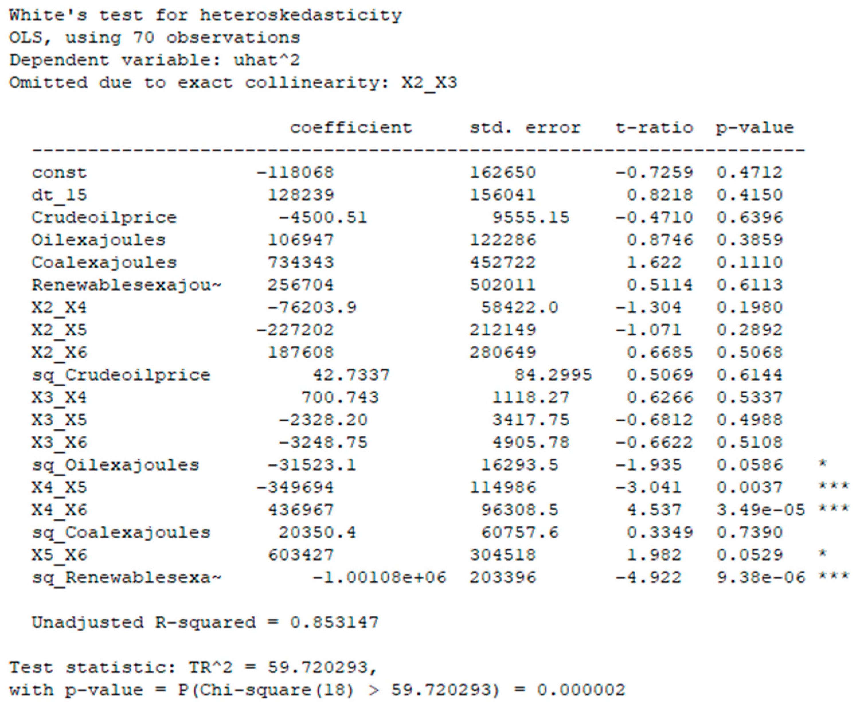
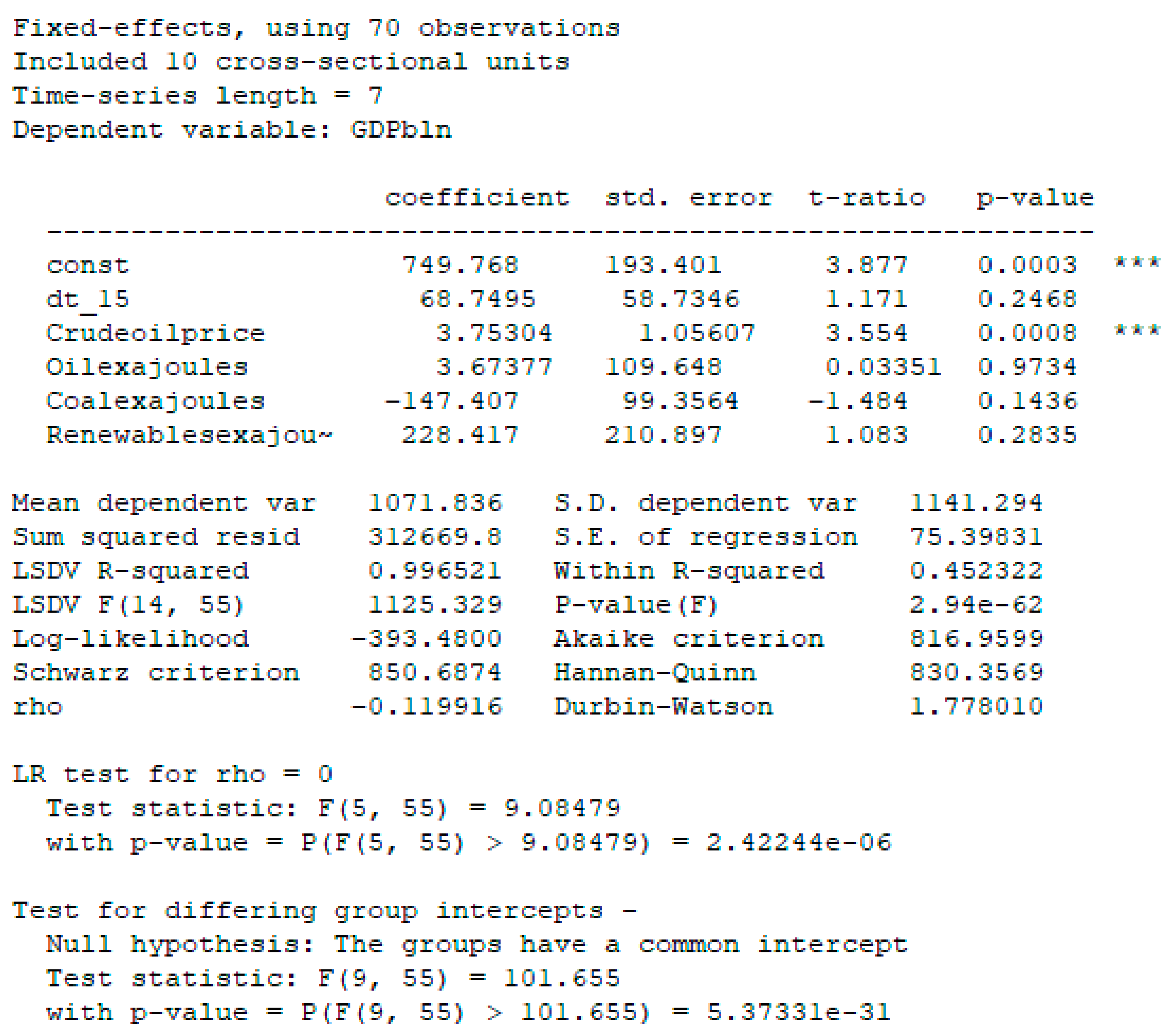
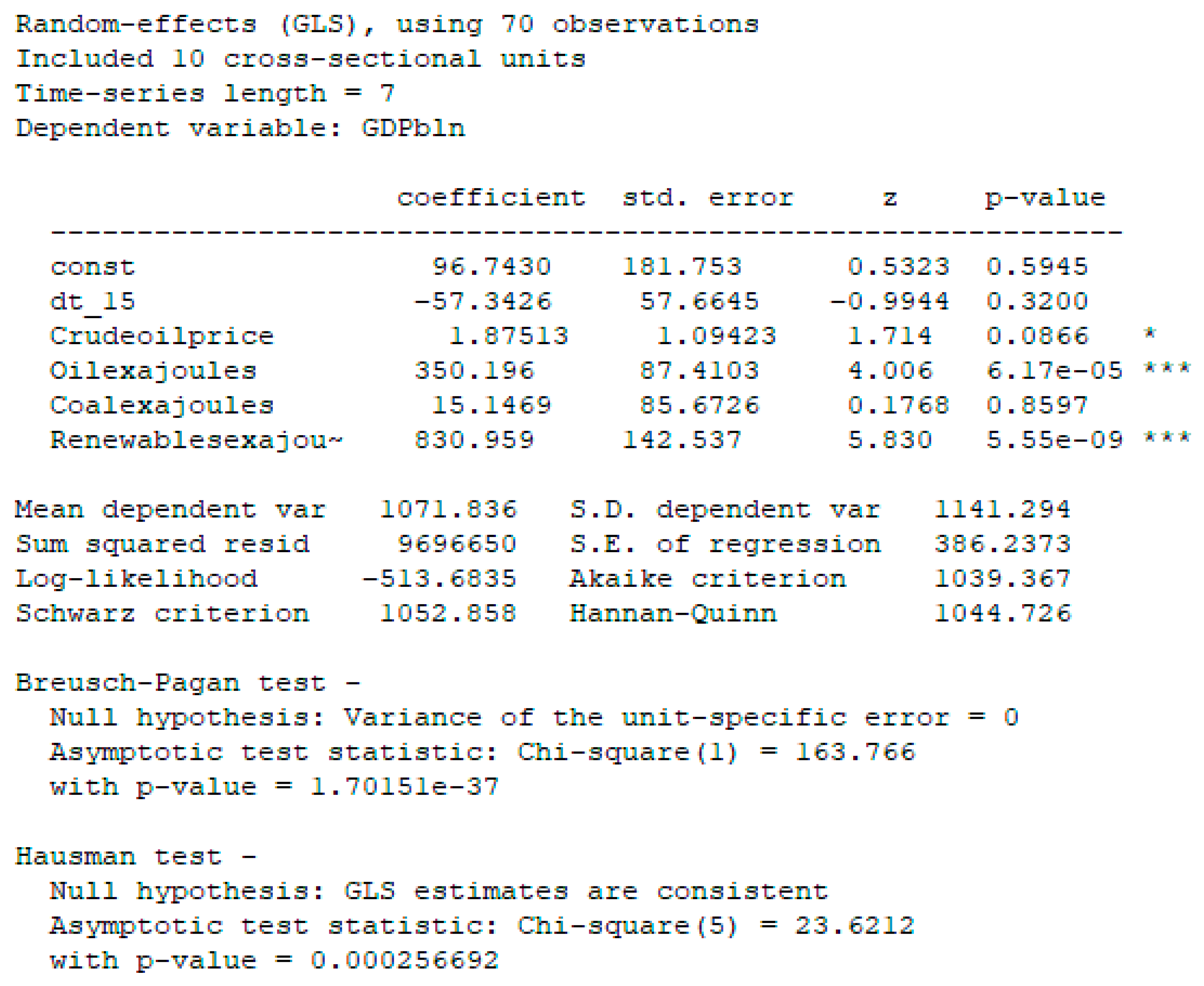
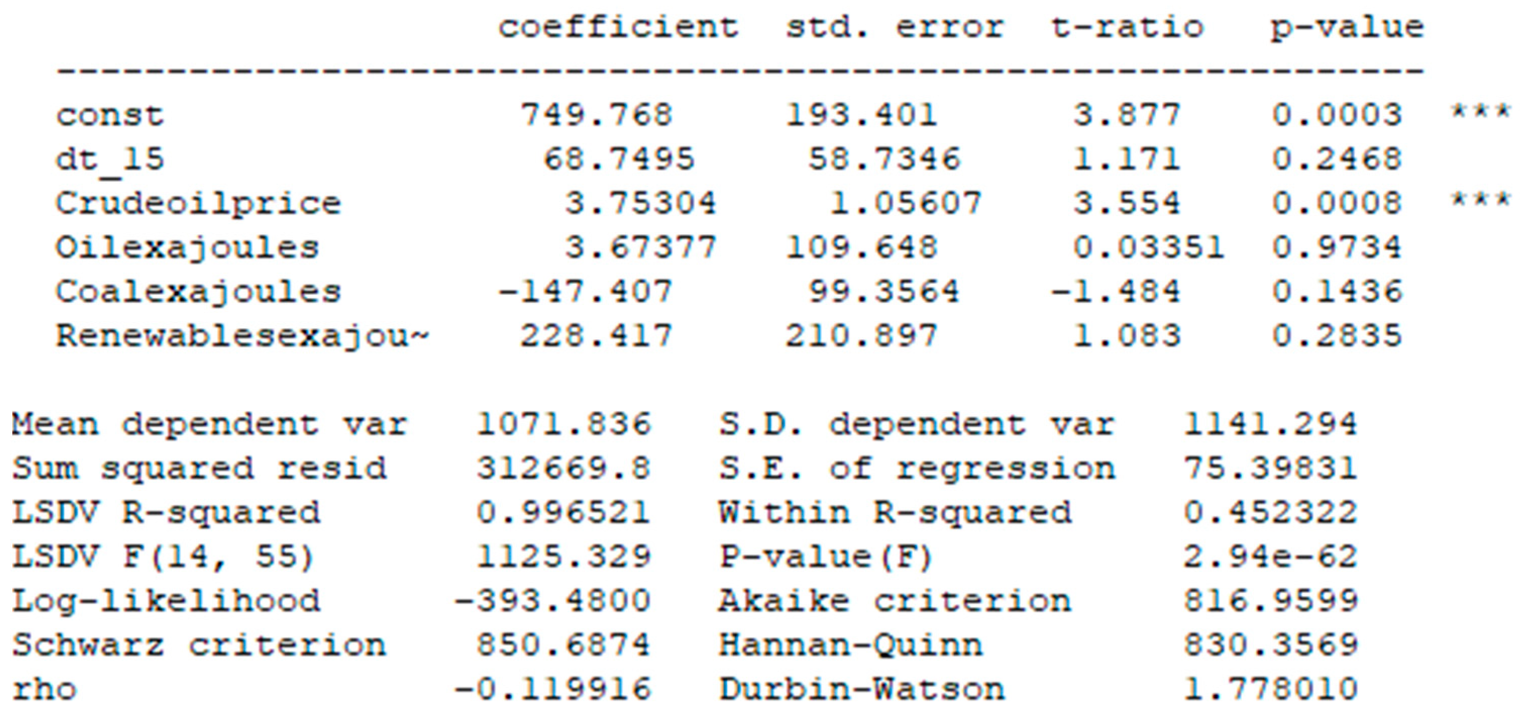
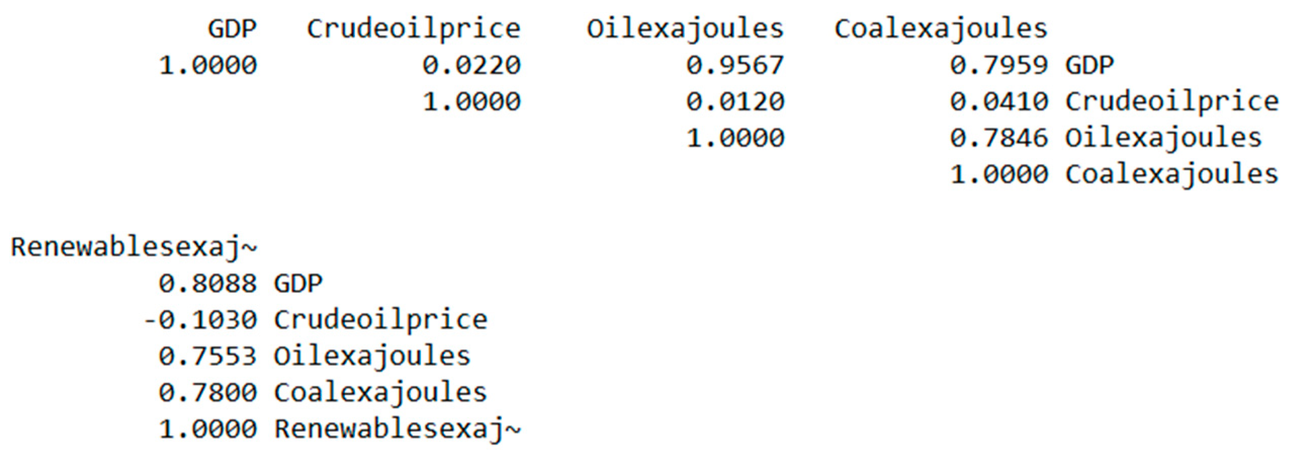
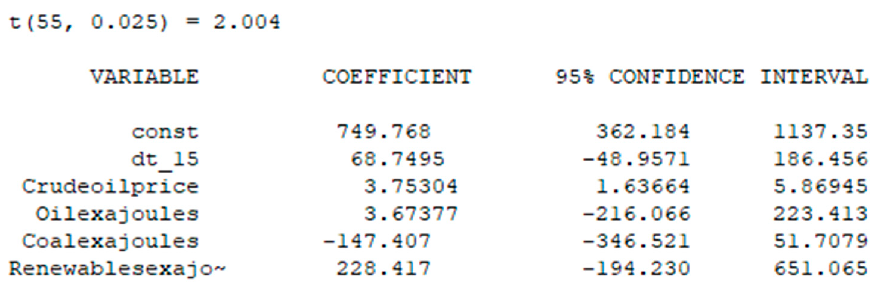
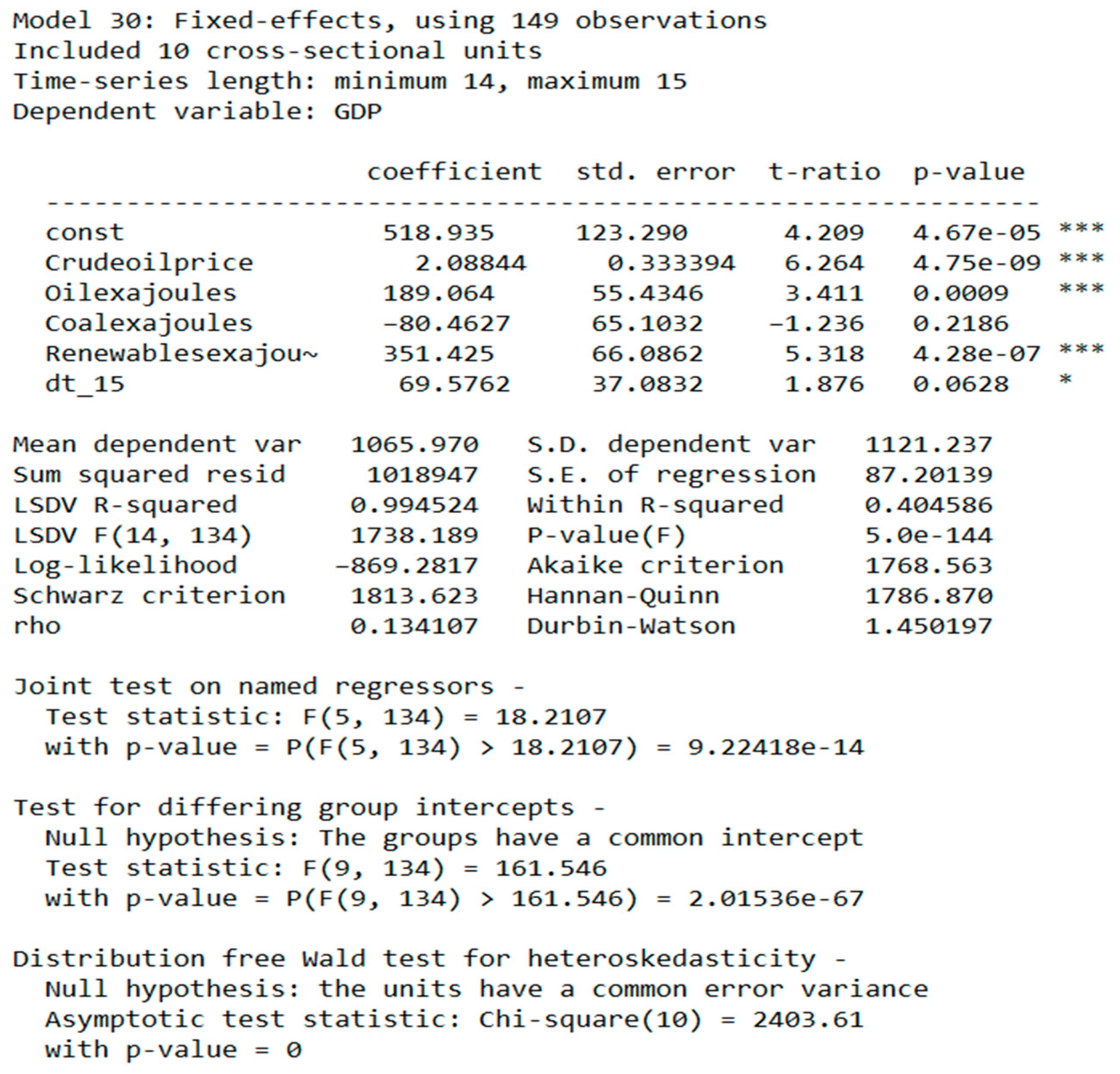
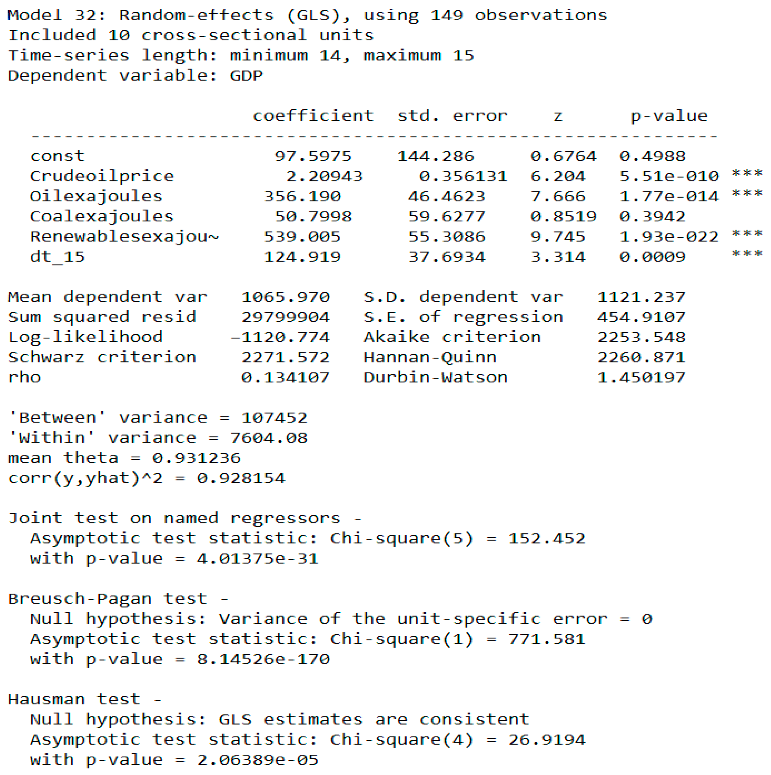
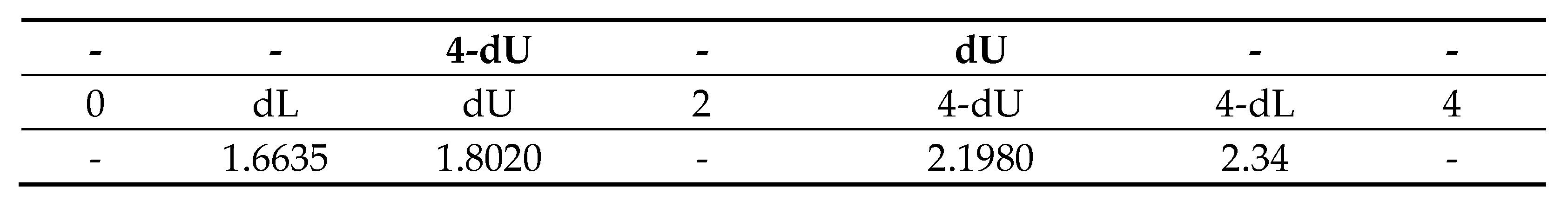
2.2. Analysis of the Model Received
2.3. Simulation Results and Their Discussion

- Oilprice—Crude oil price.
- Oil(ex)—oil consumption (exajoules).
- Coal(ex)—coal consumption (exajoules).
- Renewables (ex)—renewable energy consumption (exajoules).
- Dt15—time dummy variable (for 2020 COVID pandemic).
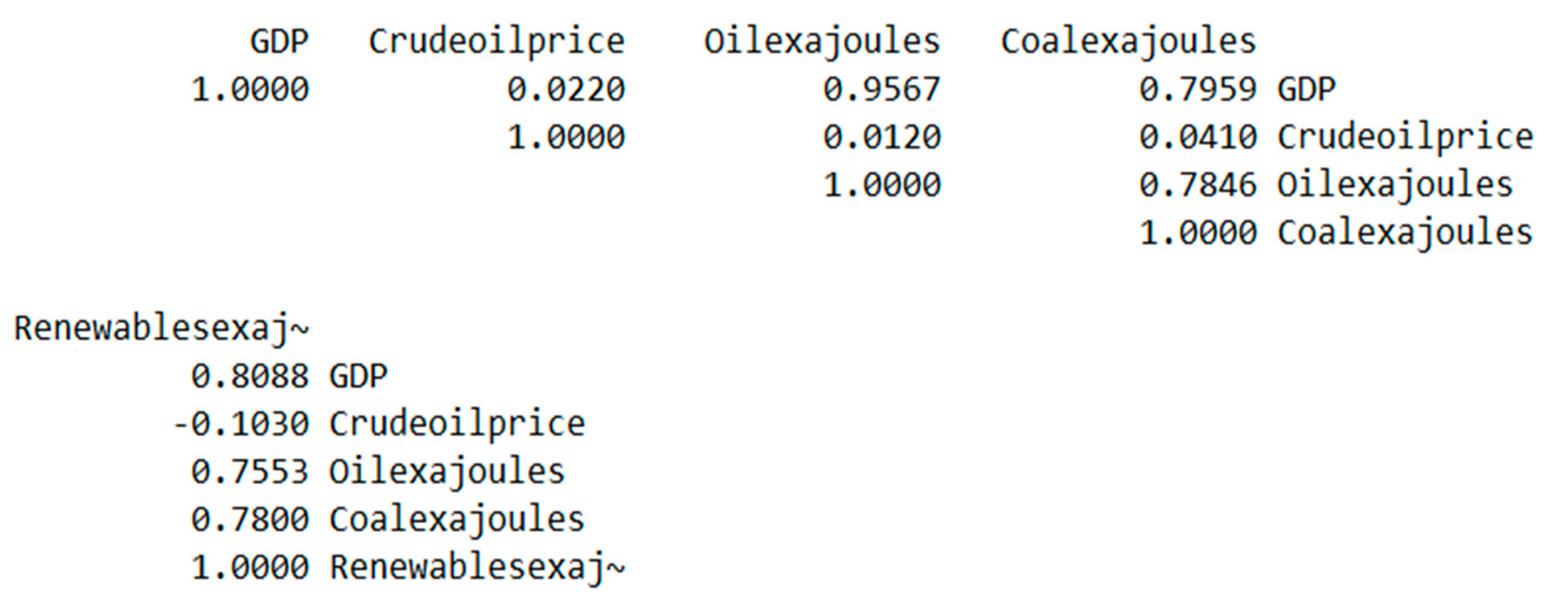
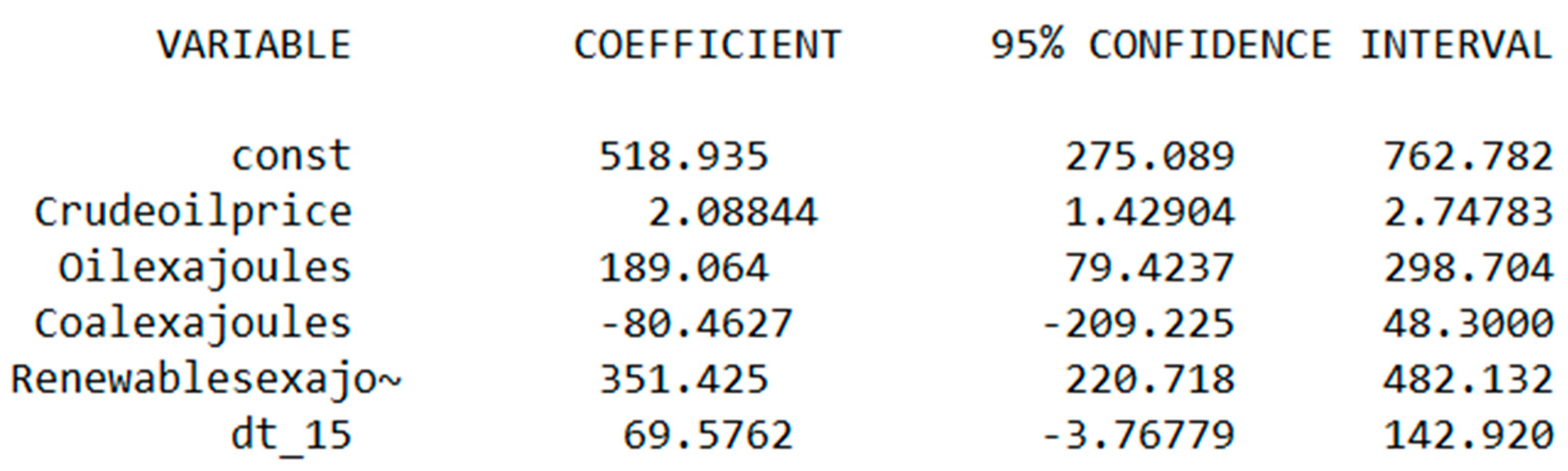
- In the period from 2014 to 2020, alternative energy played a higher role, and therefore it was a significant variable. At the same time, the volatility of oil prices and its consumption were still important for the economic growth of countries.
- Changes in oil prices, consumption of oil, and renewables positively influenced the value of GDP of given countries (Austria, Belgium, Germany, Finland, France, Netherlands, Portugal, Romania, Spain, Sweden).
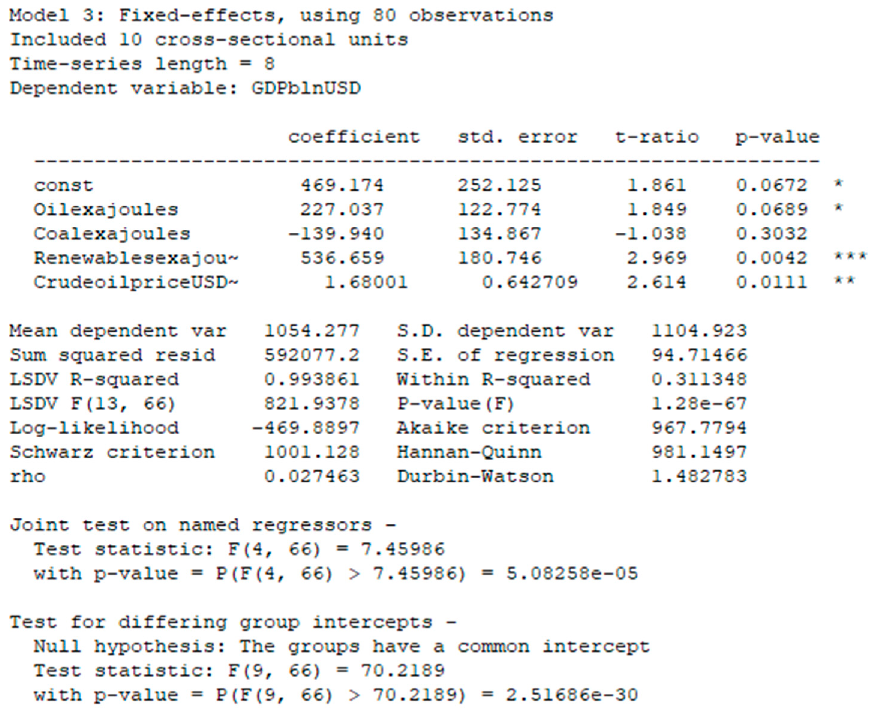
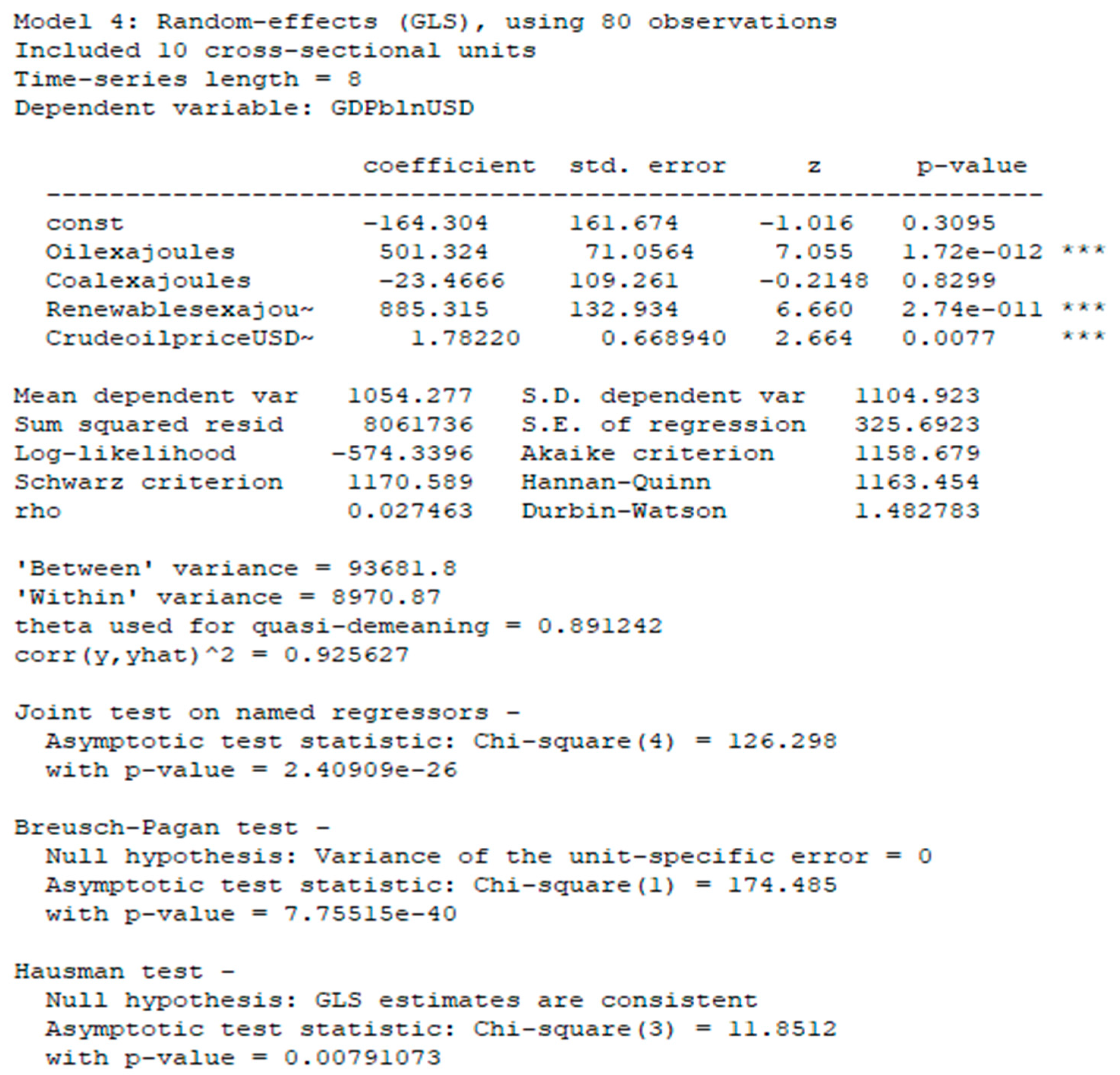
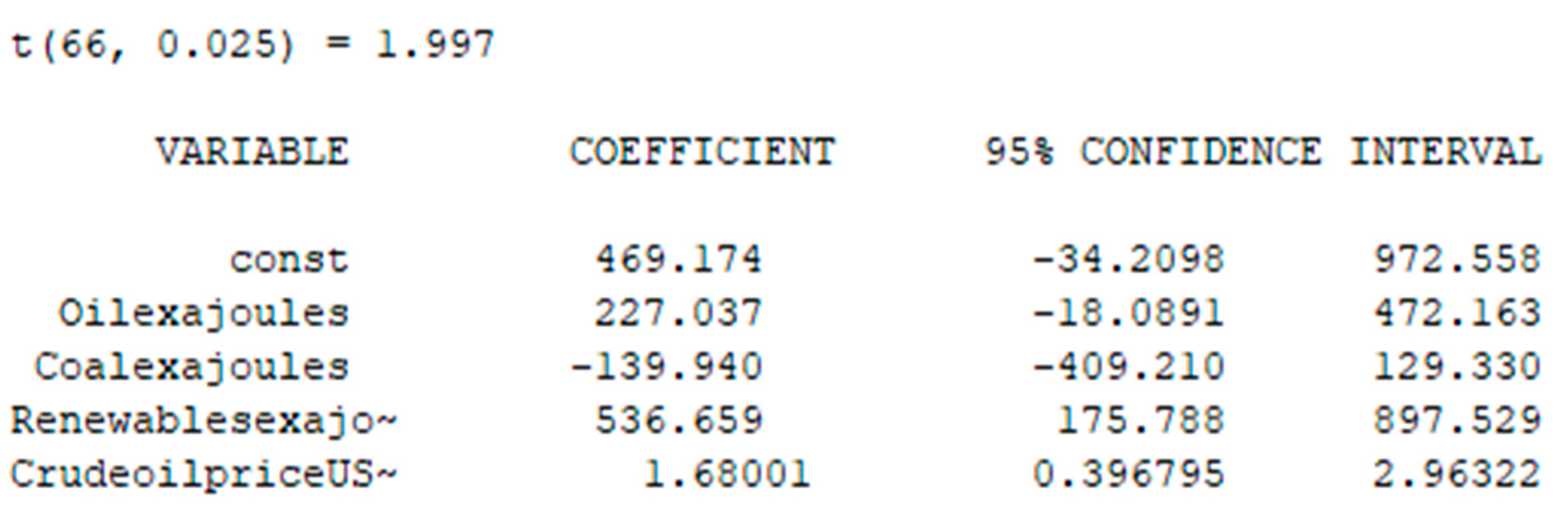
3. Simulation Results
- Oilprice—Crude oil price.
- Oil(ex)—oil consumption (exajoules).
- Coal(ex)—coal consumption (exajoules).
- Renewables (ex)—renewable energy consumption (exajoules).
- Dt15—time dummy variable (for 2020 COVID pandemic).
4. Discussion
5. Conclusions and Recommendations
Author Contributions
Funding
Institutional Review Board Statement
Data Availability Statement
Conflicts of Interest
References
- Burcu, O. Nuclear Energy-Economic Growth Nexus in OECD Countries: A Panel Data Analysis. Int. J. Econ. Perspect. 2017, 11, 138–154. [Google Scholar]
- Dynan, K.; Sheiner, L. GDP as a Measure of Economic Well–being. In Hutchins Center Working Paper 43; The Brookings Institution: Washington, DC, USA, 2018; p. 4. [Google Scholar]
- Rehman Khan, Z.Y.; Belhadi, A.M. Investigating the effects of renewable energy on international trade and environmental quality. J. Environ. Manag. 2020, 272, 15. [Google Scholar]
- Raduzzi, R. The macroeconomics outcome of oil shocks in the small Eurozone economies. World Econ. 2019, 43, 191–211. [Google Scholar] [CrossRef]
- Rafindadi, A. Impacts of renewable energy consumption on the German economic growth: Evidence from combined cointegration test. Renew. Sustain. Energy Rev. 2017, 75, 1130–1141. [Google Scholar] [CrossRef]
- Awrejcewicz, J.; Krysko, V.A.; Kutepov, I.E.; Vygodchikova, I.Y. Quantifying chaos of curvilinear beam via exponents. Commun. Non-Linear Sci. Numer. Simul. 2015, 27, 81–92. [Google Scholar] [CrossRef]
- Vazquez, P.V. Estimation of the potential effects of offshore wind on the Spanish economy. Renew. Energy 2017, 111, 815–824. [Google Scholar] [CrossRef]
- Baldoni, E.; Coderoni, S.; di Giuseppe, E.; D’orazio, M.; Esposti, R.; Maracchini, G. A software tool for a stochastic life cycle assessment and costing of buildings’ energy efficiency measures. Sustainability 2021, 13, 7975. [Google Scholar] [CrossRef]
- Borodin, A.; Zaitsev, V.; Mamedov, Z.F.; Panaedova, G.; Kulikov, A. Mechanisms for Tax Regulation of CO2-Equivalent Emissions. Energies 2022, 15, 7111. [Google Scholar] [CrossRef]
- Tong, D.; Zhang, Q.; Zheng, Y.; Caldeira, K.; Shearer, C.; Hong, C.; Qin, Y.; Davis, S.J. Committed Emissions from Existing Energy Infrastructure Jeopardize 1.5 °C Climate Target. Nature 2019, 572, 373–377. [Google Scholar] [CrossRef]
- Sobamowo, G.M.; Ojolo, S.J. Techno-economic analysis of biomass energy utilization through gasification technology for sustainable energy production and economic development in Nigeria. Energy 2018, 2018, 4860252. [Google Scholar] [CrossRef] [Green Version]
- Levi-Oguike, J.; Sandoval, D.; Ntagwirumugara, E. A Comparative Life Cycle Investment Analysis for Biopower Diffusion in Rural Nigeria. Sustainability 2022, 14, 1423. [Google Scholar] [CrossRef]
- Breusch, T.S.; Pagan, A.R. A Simple Test for Heteroscedasticity and Random Coefficient Variation. Econometrica 1979, 47, 1287–1294. [Google Scholar] [CrossRef]
- Subbotin, Y.; Shevaldin, V. On one method of constructing local parabolic splines with additional nodes. Proc. Inst. Math. Mech. Ural. Branch Russ. Acad. Sci. 2019, 25, 205–219. [Google Scholar]
- Halunga, A.; Orme, C.; Yamagata, T. A Heteroskedasticity Robust Breusch-Pagan Test for Contemporaneous Correlation in Dynamic Panel Data Models. J. Econom. 2017, 198, 209–230. [Google Scholar] [CrossRef] [Green Version]
- Tao, L.; Chen, Y.; Liu, X.; Wang, X. An integrated multiple criteria decision making model applying axiomatic fuzzy set theory. Appl. Math. Model. 2012, 36, 5046–5058. [Google Scholar] [CrossRef]
- Büscher, C.; Ufer, U. The (Un)availability of Human Activities for Social Intervention: Reflecting on Social Mechanisms in Technology Assessment and Sustainable Development Research. Sustainability 2022, 14, 1394. [Google Scholar] [CrossRef]
- Powell, D.J.; Romero, D.; Gaiardelli, P. New and Renewed Manufacturing Paradigms for Sustainable Production. Sustainability 2022, 14, 1279. [Google Scholar] [CrossRef]
- Arellano, M.; Bover, O. Another look at the instrumental variables estimation of error components models. J. Econom. 1995, 68, 29–51. [Google Scholar] [CrossRef] [Green Version]
- Lu, T. A Fuzzy Network DEA Approach to the Selection of Advanced Manufacturing Technology. Sustainability 2021, 13, 4236. [Google Scholar] [CrossRef]
- Mamedov, Z.F.; Qurbanov, S.H.; Streltsova, E.; Borodin, A.; Yakovenko, I.; Aliev, A. Mathematical models for assessing the investment attractiveness of oil companies. SOCAR Proc. 2021, 4, 102–114. [Google Scholar] [CrossRef]
- Wu, Z.; Zhao, Z.; Niu, G. Introduction to the Popular Open Source Statistical Software (OSSS); Open Source Software for Statistical Analysis of Big Data; Bryant University: Smithfield, RI, USA, 2020. [Google Scholar]
- Borodin, A.; Panaedova, G.; Ilyina, I.; Harputlu, M.; Kiseleva, N. Overview of the Russian Oil and Petroleum Products Market in Crisis Conditions: Economic Aspects, Technology and Problems. Energies 2023, 16, 1614. [Google Scholar] [CrossRef]
- Kisswani, A.; Kisswani, K. Modeling the employment–oil price nexus: A non-linear cointegration analysis for the U.S. market. J. Int. Trade Econ. Dev. 2019, 28, 1–17. [Google Scholar] [CrossRef]
- Fatima, T.; Mentel, G.; Doğan, B.; Hashim, Z.; Shahzad, U. Investigating the role of export product diversifcation for renewable, and non-renewable energy consumption in GCC (gulf cooperation council) countries: Does the Kuznets hypothesis exist? Environ. Dev. Sustain. 2022, 24, 8397–8417. [Google Scholar] [CrossRef] [PubMed]
- Alzaid, A.; Al-Osh, M.A. First-Order Integer-Valued Autoregressive (INAR (1)) Process: Distributional and Regression Properties. Stat. Neerl. 1988, 42, 53–61. [Google Scholar] [CrossRef]
- Brown, R.P.C.; Carmignani, F.; Fayad, G. Migrants’ remittances and financial development: Macro- and micro-level evidence of a perverse relationship. World Econ. 2013, 36, 636–660. [Google Scholar] [CrossRef]
- Steutel, F.W.; van Harn, K. Discrete Analogues of Self-Decomposability and Stability. Ann. Probab. 1979, 7, 893–899. [Google Scholar] [CrossRef]
- Lima, V.; Souza, T.; Cribari-Neto, F.; Fernandes, G. Heteroskedasticity-robust inference in linear regressions. Comm. Statist. Simulation Comput. 2009, 39, 194–206. [Google Scholar] [CrossRef]
- Sovacool, B.K.; Schmid, P.; Stirling, A.; Walter, G.; MacKerron, G. Differences in carbon emissions reduction between countries pursuing renewable electricity versus nuclear power. Nat. Energy 2020, 5, 928–935. [Google Scholar] [CrossRef]
- Değirmen, S.; Saltık, Ö. Could Nuclear Energy Production and Economic Growth Relationship for Developed Countries Be an Incentive for Developing Ones?: A Panel ARDL Evidence Including Cointegration Analysis; GELISIM-UWE 2019 Special Issue, İstanbul Gelişim Üniversitesi Sosyal Bilimler Dergisi; Mersin University: Mersin, Turkey, 2019; pp. 1–28. [Google Scholar] [CrossRef]
- Hausman, J.A. Specification Tests in Econometrics. Econometrica 1978, 46, 1251–1271. [Google Scholar] [CrossRef] [Green Version]
- Greene, W. Fixed and Random Effects in Stochastic Frontier Models. J. Product. Anal. 2005, 23, 7–32. Available online: http://www.jstor.org/stable/41770178 (accessed on 8 February 2023). [CrossRef] [Green Version]
- deHaan, E. Using and Interpreting Fixed Effects Models. 2021. Available online: https://papers.ssrn.com/sol3/papers.cfm?abstract_id=3699777 (accessed on 8 February 2023).
- Lepore, D.; Micozzi, A.; Spigarelli, F. Industry 4.0 Accelerating Sustainable Manufacturing in the COVID-19 Era: Assessing the Readiness and Responsiveness of Italian Regions. Sustainability 2021, 13, 2670. [Google Scholar] [CrossRef]
- Basu, A.; Mandal, A.; Mart´ın, N.; Pardo, L. Generalized Wald-type tests based on minimum density power divergence estimators. Statistics 2016, 50, 1–26. [Google Scholar] [CrossRef]
- Borodin, A.; Mityushina, I.; Harputlu, M.; Kiseleva, N.; Kulikov, A. Factor Analysis of the Efficiency of Russian Oil and Gas Companies. Int. J. Energy Econ. Policy 2023, 13, 172–188. [Google Scholar] [CrossRef]
- Lee, C. Adkins, Using gretl for Monte Carlo experiments. J. Appl. Econom. 2010, 5, 880–885. [Google Scholar]
- Segarra-Blasco, A.; Teruel, M.; Cattaruzzo, S. The economic reaction to non-pharmaceutical interventions during Covid-19. Econ. Anal. Policy 2021, 72, 592–608. [Google Scholar] [CrossRef]
- COVID-19. European Centre for Disease Prevention and Control. Published 2021. Available online: https://www.ecdc.europa.eu/en (accessed on 14 January 2022).
- Hale, T.; Angrist, N.; Goldszmidt, R.; Kira, B.; Petherick, A.; Phillips, T. A global panel database of pandemic policies (Oxford COVID-19 Government Response Tracker). Nat. Hum. Behav. 2021, 5, 529–538. [Google Scholar] [CrossRef]
- Claeson, M.; Hanson, S. COVID-19 and the Swedish enigma. Lancet 2021, 397, 259–261. [Google Scholar] [CrossRef]
- Olagnier, D.; Mogensen, T.H. The COVID-19 pandemic in Denmark: Big lessons from a small country. Cytokine Growth Factor Rev. 2020, 53, 10–12. [Google Scholar] [CrossRef]
- Mamedov, Z.F.; Qurbanov, S.H.; Streltsova, E.; Borodin, A.; Yakovenko, I.; Aliev, A. Assessment of the potential for sustainable development of electric power enterprises: Approaches, models, technologies. SOCAR Proc. 2022, 2, 15–27. [Google Scholar] [CrossRef]
- Borodin, A.; Natocheeva, N.; Khominich, I.; Kulikov, A.; Shchegolevatykh, N. The Impact of the Business Environment on the Effectiveness of the Implementation of the Financial Strategy of the Oil and Gas Company. Int. J. Energy Econ. Policy 2021, 11, 13–21. [Google Scholar] [CrossRef]


Disclaimer/Publisher’s Note: The statements, opinions and data contained in all publications are solely those of the individual author(s) and contributor(s) and not of MDPI and/or the editor(s). MDPI and/or the editor(s) disclaim responsibility for any injury to people or property resulting from any ideas, methods, instructions or products referred to in the content. |
© 2023 by the authors. Licensee MDPI, Basel, Switzerland. This article is an open access article distributed under the terms and conditions of the Creative Commons Attribution (CC BY) license (https://creativecommons.org/licenses/by/4.0/).
Share and Cite
Aliev, A.; Magomadova, M.; Budkina, A.; Harputlu, M.; Yusifova, A. EU: The Effect of Energy Factors on Economic Growth. Energies 2023, 16, 2908. https://doi.org/10.3390/en16062908
Aliev A, Magomadova M, Budkina A, Harputlu M, Yusifova A. EU: The Effect of Energy Factors on Economic Growth. Energies. 2023; 16(6):2908. https://doi.org/10.3390/en16062908
Chicago/Turabian StyleAliev, Ayaz, Madina Magomadova, Anna Budkina, Mustafa Harputlu, and Alagez Yusifova. 2023. "EU: The Effect of Energy Factors on Economic Growth" Energies 16, no. 6: 2908. https://doi.org/10.3390/en16062908