A Numerical Model for Pressure Analysis of a Well in Unconventional Fractured Reservoirs

Abstract

Fractured reservoirs are highly heterogeneous in both matrix and fracture properties, which results in significant variations in well production. Assessing and quantifying the influence of fractures on fluid flow is essential for developing unconventional reservoirs. The complicated effects of fractures in unconventional fractured reservoirs on fluid flow highly depend on fracture geometry, fracture distribution, and fracture properties, which can be reflected in pressure transient testing. The biggest challenge lies in delineating the pre-existing natural fracture distribution pattern, density, azimuth, and connectivity. Using the advanced finite element method, this paper builds a finely characterized near-wellbore model to numerically simulate the pressure transient testing process in naturally fractured reservoirs and further evaluates fracture-related effects to obtain a more accurate solution. First, the numerical program is benchmarked by the analytical solutions and numerical results of Eclipse. Next, different fracture models with single fractures or fracture networks are set up to investigate the effects of fracture parameters numerically (e.g., fracture location, fracture dip angle, fracture spacing, the ratio of fracture permeability to matrix permeability, fracture network orientation, horizontal fracture distribution, etc.) on pressure transient behaviors in naturally fractured reservoirs. Velocity and pressure profiles are presented to visualize and analyze their effects, and new features in the flow regimes of the derivative plots of the bottom-hole pressure are identified and discussed. Finally, based on geological and geophysical data, including image logs, core descriptions, wireline logs, and seismic and well test data, a practical fractured model of the Dalwogan 2 well in the Surat basin is built, analyzed, and compared with homogenous and measured data. The results show significance in characterizing the complex fracture networks in near-wellbore models of unconventional fractured reservoirs.

1. Introduction

The high degree of uncertainty involved in the development of unconventional fractured reservoirs leads to the need to understand the flow behavior in reservoirs [1]. Generally, fractures serve as both storage spaces and the main flow channels in reservoir rocks [2]. Fractures control the storage, impact the distribution of the natural gas storage in reservoirs, and provide necessary information related to tectonics, overpressure, burial history, and diagenesis [3,4]. The fluctuation of well production in fractured reservoirs is caused by the extreme heterogeneity of the matrix and fractures, and a large proportion of the production might come from a short, intensely fractured interval within a single well [5]. Research on fractures in actual unconventional reservoirs has received attention [6,7]. Therefore, improving the understanding of fracture characteristics is critical for the efficient development of unconventional fractured reservoirs, such as carbonate reservoirs.

Various methods are used for fracture identification in reservoirs. (1) Direct observation of fracture-based well cores and natural outcrops is used, but cost constraints affect the number of implementations [8]. (2) Fracture identification using new seismic methods based on pre-stacked seismic data has emerged based on the principles of amplitude variation with azimuth [9,10], travel-time variation with azimuth [11], and velocity variation with azimuth [12], and fracture proximity, thinned fault likelihood, fracture density [13], and post-stack reflective seismic waves [14,15]. Each method provides fracture information on a different scale and has its own limitations. (3) Fracture classification and prediction through artificial intelligence and machine learning methods. Conventional logging, downhole videos, and image logging are all tools used in fracture identification [7,16]. The geological characteristics of fractures, including fracture density, fracture spacing, and fracture conductivity, can present many features of the flow in naturally fractured reservoirs. Furthermore, seismic wave attenuation, which is closely related to fracture properties because of its scattering and fluid-related mechanisms [17], can be used to detect fractures and define their orientation, density, and fluid content in carbonate rocks [18]. However, the biggest challenge lies in delineating the pre-existing natural fracture distribution pattern, density, azimuth, and connectivity [19]. While the mechanics and geologic conditions that generate natural fractures are generally well understood, the actual complex characteristics of unconventional fractured reservoirs cannot be accurately described. Therefore, further research is needed to better characterize fractures in unconventional fractured reservoirs. Fracture parameters, including fracture location, fracture spacing, the ratio of fracture permeability to matrix permeability, fracture network orientation, and fracture dip angle, have rarely been investigated and are researched in detail in this paper.

The properties of fractures at the meter scale are mostly characterized by using pressure transient testing, which is also widely used to estimate reservoir pressure, reservoir permeability, and wellbore conditions (e.g., well completion, wellbore damage, and wellbore storage) and detect faults and sealing boundaries in conventional oil and gas wells by observing the pressure responses resulting from the change in the production rate [20,21]. However, the conventional pressure transient testing method is proposed based on the assumptions of a single-phase flow in a homogeneous infinite reservoir with constant fluids and reservoir properties. These assumptions are obviously not suitable for unconventional fractured reservoirs that have complex fractures at various scales with different fracture distributions, fracture spacings, fracture conductivities, fracture orientations, and fracture geometries. Therefore, the utility of pressure transient testing to obtain the properties of fractures in unconventional fractured reservoirs is a challenge for petroleum engineers. Pressure transient testing interpretation for unconventional fractured reservoirs is quite difficult due to the existence of complex fracture networks, which give rise to the appearance of numerous complex flow regimes reflected in pressure transient testing data. The classical pressure transient analysis for fractured reservoirs is based on the dual porosity model [22], which causes a distinct “V”-shape in the middle time region of the pressure derivative [23,24,25]. This is due to recharge, which occurs because the fluids in the fractures are produced at a faster rate than they are replaced from the matrix [26]. Classical theory predicts that this recharge effect increases with increasing fracture-matrix permeability contrast and that the width and depth of the “V” in the pressure transient allow us to back-calculate the fracture-matrix permeability contrast and the difference in fluids stored in the fracture and matrix [23,24]. Numerous research outcomes about a specific topic—the effects of fractures on pressure transient testing behaviors—have been published. Nobakht, Clarkson, and Kaviani [27] discussed the effects of reservoir types and induced hydraulic fracturing geometries. A series of type curves were developed to capture the flow regimes for various horizontal well lengths, fracture numbers, fracture lengths, and fracture spacings. Kuchuk and Biryukov [28,29] proposed a semianalytical method to investigate the pressure transient behaviors of continuously and discretely naturally fractured reservoirs and found that more than ten flow regimes may exist in fractured reservoirs. Deng et al. [30] presented an analytical solution for a fractured well with an eccentric well location in composite reservoirs and considered the well location and multi-region radial composite systems of a fully or partially penetrating fractured well. Chen et al. [31] presented an efficient semianalytical model for pressure-transient analysis in fractured wells by considering arbitrarily distributed fracture networks. Liu et al. [32,33] proposed a discrete fracture–matrix method based on a numerical well testing model to study the pressure transient behavior of discretely distributed natural fractures in a 2D reservoir. Additionally, in their sensitivity analysis, the “dip” on the pressure derivative is an important signal to identify the properties and the impacts of natural fractures. However, because of the limitations of existing analytical and semianalytical methods, most of the considered fracture characteristics are simplified, and some new features of the flow regimes identified in the derivative plots in naturally fractured low-permeability reservoirs could not be described and clarified clearly [34,35]. Numerical well testing is an effective tool to solve this problem [36,37]. It can compute a complicated model more accurately, especially by using a finite element method-based numerical simulation that can simulate models with a variety of complex structures or fractures and flow patterns in unconventional reservoirs, such as carbonate reservoirs.

It is proposed to integrate static data, including seismic, wireline logs, core, and geological data, and dynamic data, including well test data and production data, to characterize the fractures near the wellbore at the meter scale [38]. However, most of the existing well-test models for transient analysis in fractured reservoirs, using either analytical or numerical methods, are based on continuum models or simplify the fractures to a high-permeability matrix, which cannot accurately describe the actual complex features in unconventional fractured reservoirs [37]. Therefore, further studies are needed to characterize the fracture characteristics of unconventional fractured reservoirs. This paper considers more fracture parameters in unconventional fractured reservoirs and studies their effects on reservoir seepage through numerical pressure transient tests. Based on all the collected data, an integrated near-wellbore model of coal seam gas (CSG) reservoirs was built to investigate the pressure transient behaviors of fractures and better characterize naturally fractured reservoirs in this paper. The in-house developed finite element method-based code PANDAS (Parallel Adaptive Nonlinear Deformation Analysis Software) is used in this paper for the related numerical simulation of all the proposed models [39,40,41,42]. It was first verified by comparison with the available analytical solutions and numerical results obtained from Eclipse. Then, the sensitivity of various fracture parameters on pressure transient testing behaviors in low-permeability coal seams was investigated numerically and visualized using velocity and pressure profiles. Some new features in the flow regimes of the Bourdet derivative plots of the bottom-hole pressure were presented and discussed. Finally, based on the available geological and geophysical data from the Dalwogan 2 well in the Surat Basin, including image logs, core descriptions, wireline logs, and well test data, a finely characterized fracture near-wellbore model was built and analyzed to demonstrate the necessity of further investigating the effects of fractures on pressure transient testing in low-permeability CSG reservoirs and the fine characterization of heterogeneous coal seams in geological models.

2. Numerical Modeling

A numerical simulation of the finite element method was applied to investigate the effects of fractures on pressure transient testing behaviors in near-wellbore regions of a CSG reservoir. PANDAS, an in-house finite element method-based code, is an advanced multiphysics coupling software that has been applied in various scenarios, including interacting fault system dynamics and geothermal and unconventional reservoir analysis [39,40,41,42]. The fluid module of PANDAS is extended and applied to investigate the pressure transient testing behaviors in naturally fractured low-permeability coal seams.

2.1. Equation of Continuity

It is assumed that the formation is nondeformable with constant porosity and permeability. The formation and the fluid have small and constant compressibilities. The formation is assumed to be homogeneous and isotropic in one material except for the fractures. The gravity effect in our models is negligible because the thicknesses of all models are less than 10 m. Because the focus of this paper is on the effects of fractures on pressure transient behaviors, CSG adsorption and desorption are ignored. Only the low permeability and complex fracture characteristics of CSG reservoirs are considered and analyzed here, as detailed below, using PANDAS.

For a single-phase fluid flowing in a porous medium, the differential continuity equation is written as:

$$\frac{\partial \left(\rho \varphi \right)}{\partial t}+\nabla \left(\rho v\right)=q\rho$$

(1)

where $\rho$ is fluid density; $\varphi$ is formation porosity; $v$ is fluid velocity, and $q$ is flow rate.

Darcy’s law is:

$$v=-\frac{k}{\mu }\left(\nabla P\right)$$

(2)

where k is the formation permeability; $\mu$ is the viscosity, and $P$ is the pressure.

Combining Equations (1) and (2), the equation of continuity is expressed by pressure as:

$$\frac{\partial \left(\rho \varnothing \right)}{\partial t}-\nabla \left[\frac{\rho k}{\mu }\left(\nabla P\right)\right]=\rho q$$

(3)

The inner boundary condition is a constant flow rate. The flow rate varied from negative to positive depending on the well test methods. The outer boundary condition is constant pressure in our models.

2.2. Validation of the Numerical Model

Chupin et al. [43] recommended that a near-wellbore region (approximately 10 m to 100 m) around the wellbore in a low-permeability CSG reservoir should be investigated, taking into account the flow regions of the fast-flow pressure transient testing and computing expense. In this paper, the radius of our following models was chosen as 50 m. To validate our code, a drawdown test was simulated, and the results were analyzed.

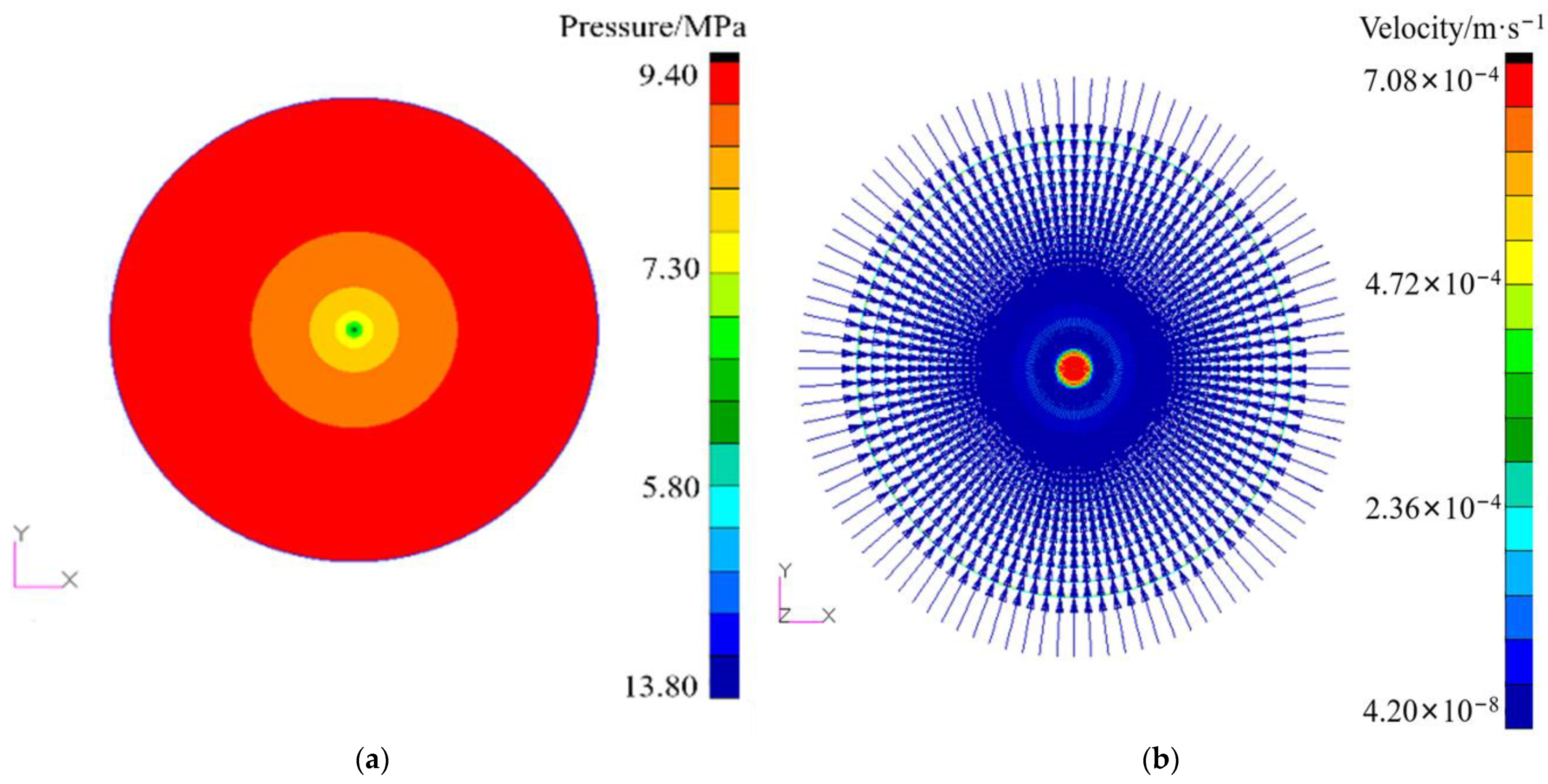
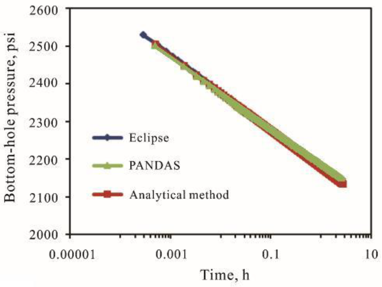
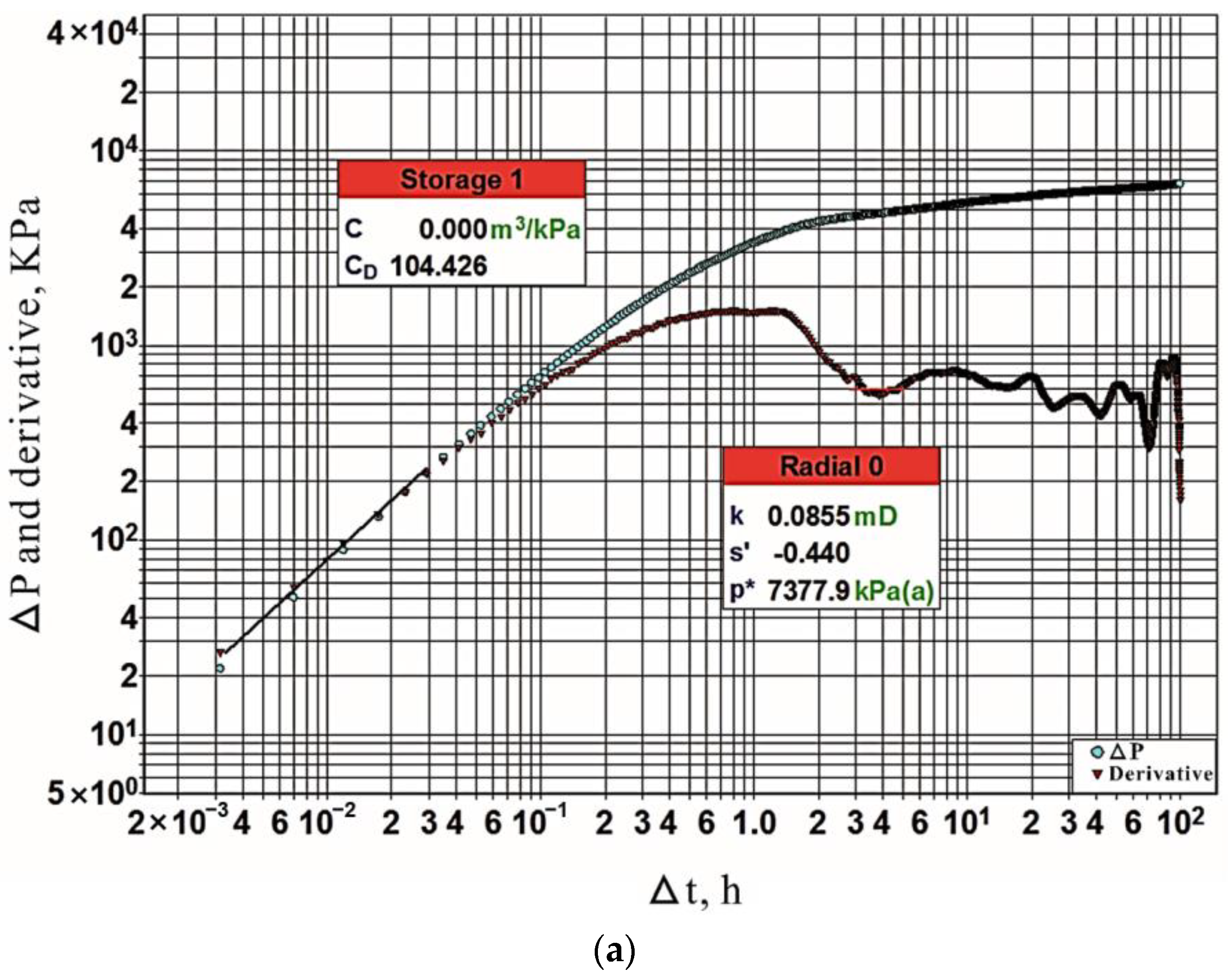
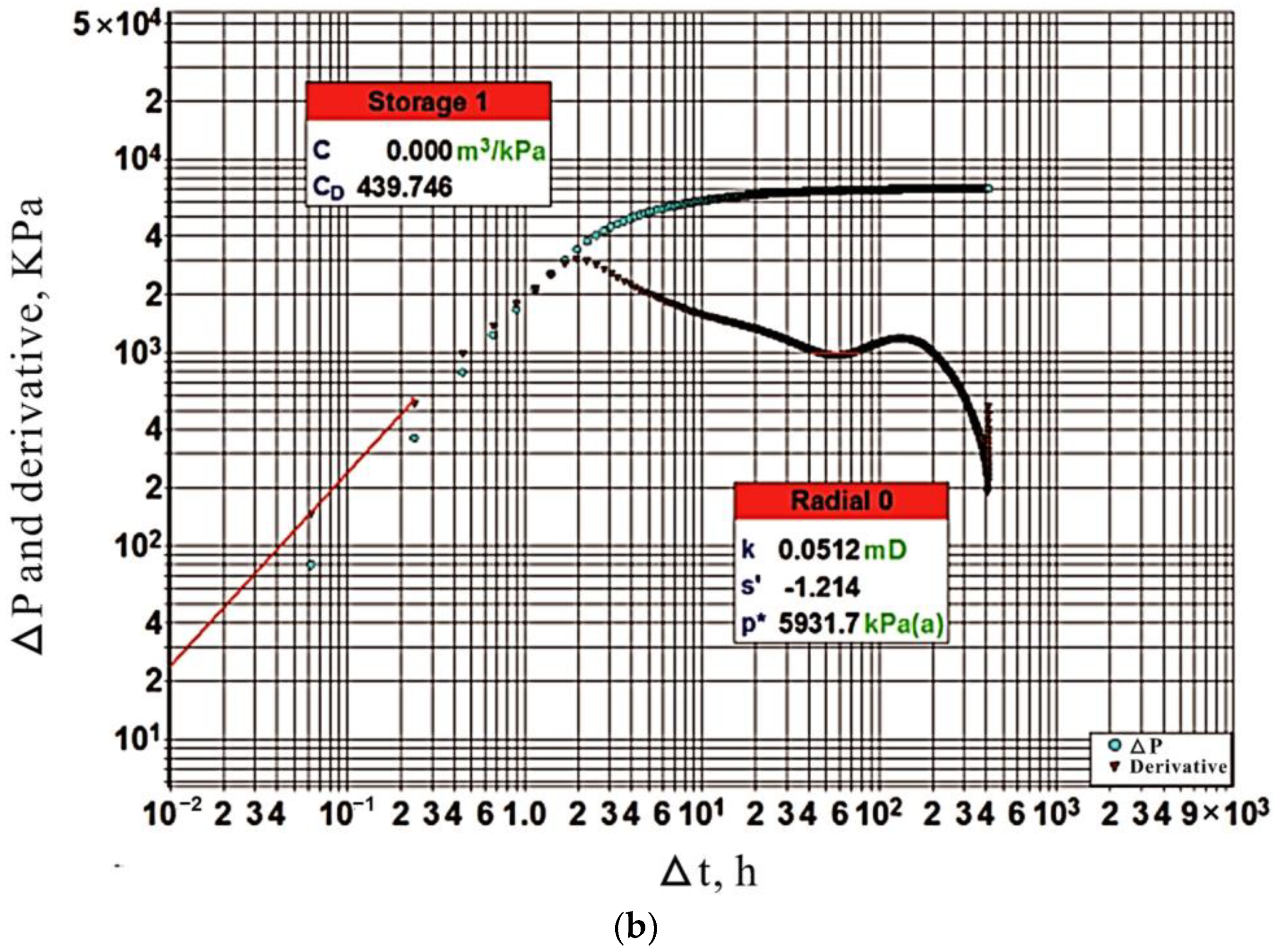
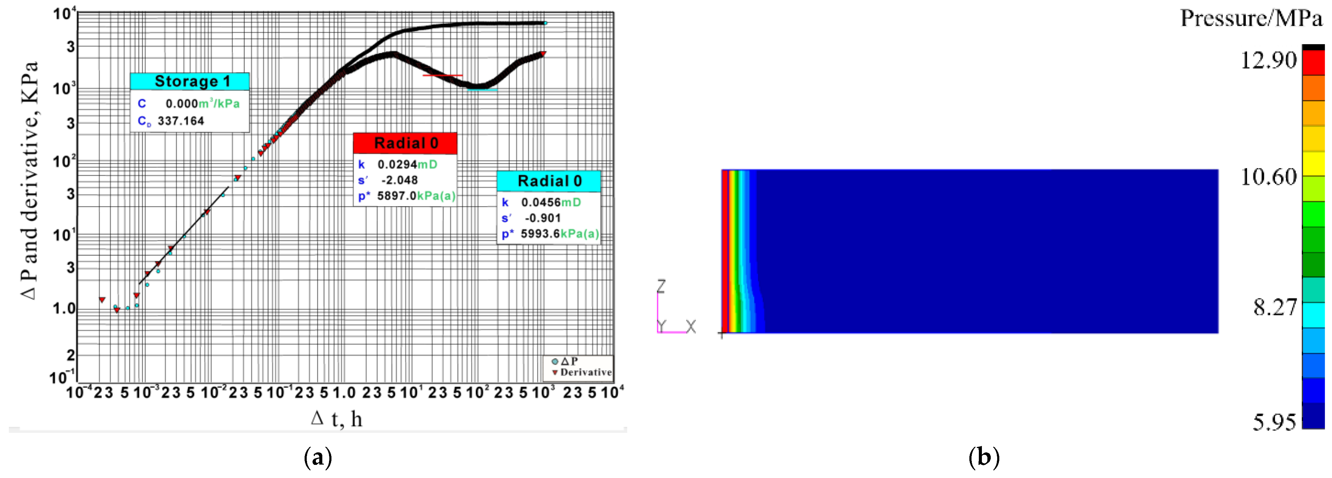
2.2.1. Bottom-Hole Pressure Validation

A numerical model was built to simulate a pressure drawdown test, and the obtained bottom-hole pressure was compared with the analytical solution and numerical results from the commercial numerical software Eclipse. The primary input data are listed in

Table 1. Well and reservoir parameters.

Parameters	Values	Parameters	Values
Wellbore radius, ft	0.25	Permeability, mD	48
Net thickness, ft	17	Reservoir pressure, psi	2810
Porosity	0.2	Formation volume factor	1.0
Compressibility, psi−1	1.0 × 10−6	Flow rate(surface), STB/D	500
Viscosity, cp	1.0

. For a more detailed description of the model, please refer to Ramey Jr. [44]. The pressure and velocity distributions at 6.5 hours are shown in Figure 1a,b.

Analytical solutions of the diffusivity equation for a pressure drawdown test in an infinite-acting reservoir can be obtained by taking the well as a line source [45]. The bottom-hole pressure $P_w$can be approximated by

$$P_w=P_i-162.6\frac{qB\mu }{kh}\left(logt+log\frac{k}{\varnothing \mu C_t{r}_w^2}+0.867S-3.2274\right)$$

(4)

where $P_i$ is the initial reservoir pressure; $B$ is the formation volume factor; $h$is the formation thickness;$C_t$ is the total compressibility of the fluid and formation, and S is the skin factor. Other parameters are the same as those introduced above. Figure 2 shows the comparison of the bottom-hole pressure change over the flow time obtained from the mentioned three methods. The result shows that during the steady-state radial flow, the numerical results from PANDAS and Eclipse and the analytical solution (Equation (4)) match each other very well.

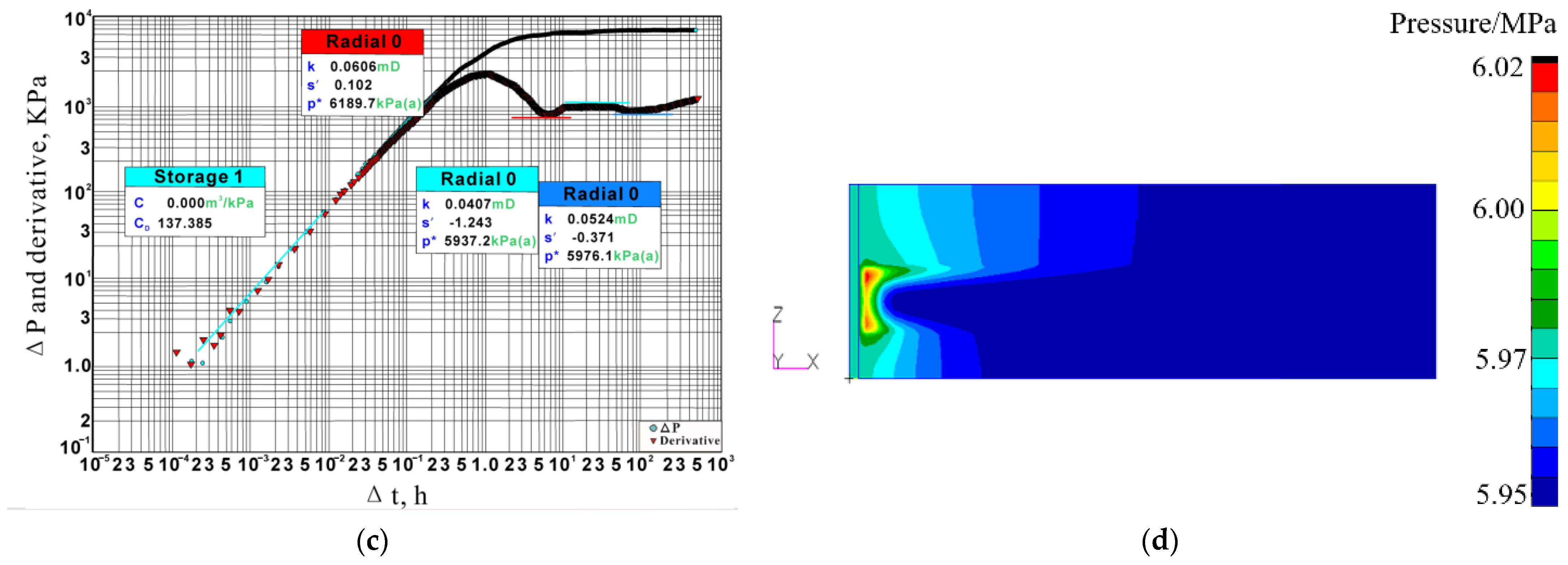
2.2.2. Permeability Calculation and Validation

After the numerical drawdown test, the reservoir permeability can be determined by analyzing the bottom-hole pressure and the production rate. If the interpreted permeability is equal to the input permeability in our model or their difference is less than 10% of the input value, the simulated results are accurate [46,47]. In log-log coordinates, based on the bottom-hole pressure difference and pressure derivative obtained by PANDAS, the radial flow regime can be identified, and then the reservoir permeability is calculated to be 48.1219 mD. The difference between the interpreted permeability and the input value is 0.1219 mD, less than 1% of 48 mD. Therefore, the simulated results from PANDAS are accurate and can be used to simulate the pressure transient testing process.

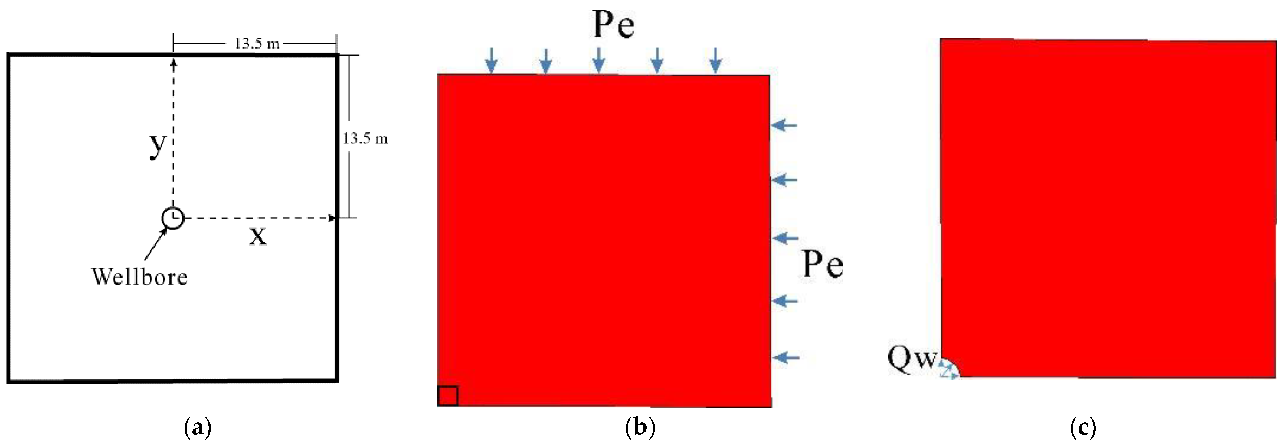
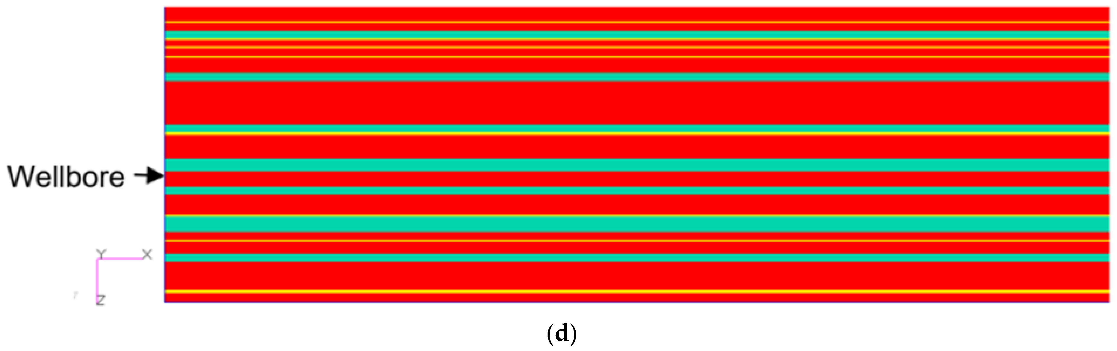
2.3. Model Parameters

When the geological conditions are complex, more grids are needed for depiction, and more computing resources are required. Therefore, a symmetrical case was assumed, and only one-fourth of the rectangular model was built to study the pressure transient behaviors of naturally fractured low-permeability coal seams in this paper to reduce the computing time and cost (Figure 3). The size of the model in the X and Y directions was 13.5 m × 13.5 m. In the following models, the inner boundaries (Qw) have a constant injection rate or no flow rate, and the outer boundaries (Pe) have a constant pressure. The initial condition is the initial reservoir pressure. The input data in the models are summarized in

Table 2. Well and reservoir parameters for all models in Section 3.

Parameters	Values	Parameters	Values
Wellbore radius, m	0.10	Matrix permeability, mD	0.048
Net thickness, m	1.90	Reservoir pressure, Pa	5.954 × 106
Porosity	0.02	Formation volume factor	1.0
Compressibility, Pa−1	3.67 × 10−11	Flow rate(surface), m3/d	0.125
Viscosity, Pa.s	1.0 × 10−3	Fracture permeability, mD	4.8
		(Unless otherwise prescribed)

. Since vertical wellbores are the most common wellbore types used for CSG development [48,49], all numerical models built in this paper are vertical wellbores.

3. Results and Discussion

3.1. Single-Fracture Parametric Study

Single fractures are the basic component of naturally fractured coal seams. Various fracture parameters, including fracture geometry, fracture location, fracture permeability relative to the matrix permeability, and fracture dip angle, affect the flow in coal seam gas reservoirs. These effects were investigated using numerical pressure transient testing in this section. Kuchuk and Biryukov [50] applied the semianalytical method to reveal and emphasize its critical effects by analyzing derivative plots. Therefore, the Bourdet derivative plots of the bottom-hole pressure were presented, and velocity and pressure profiles were used to explain the effects.

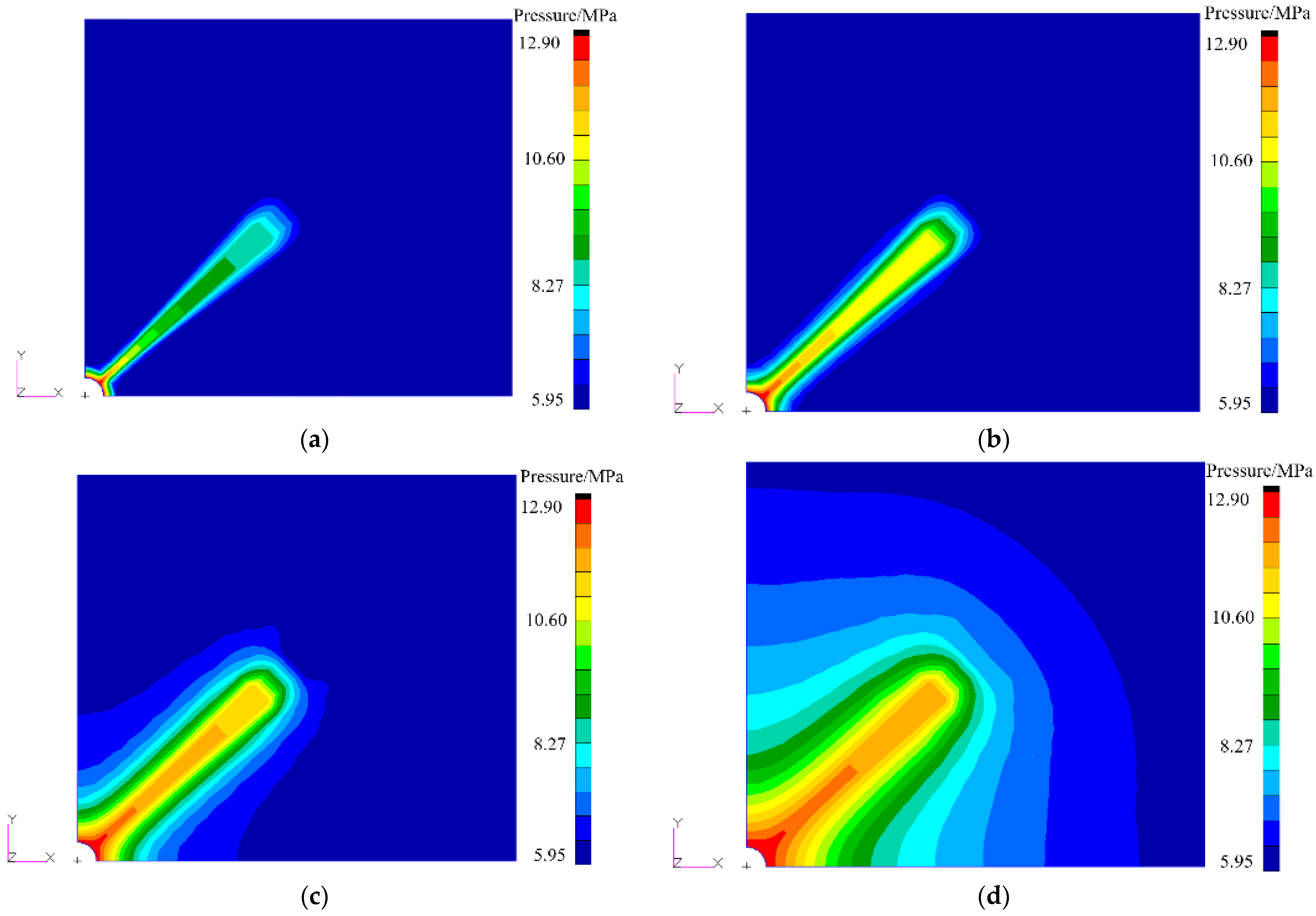
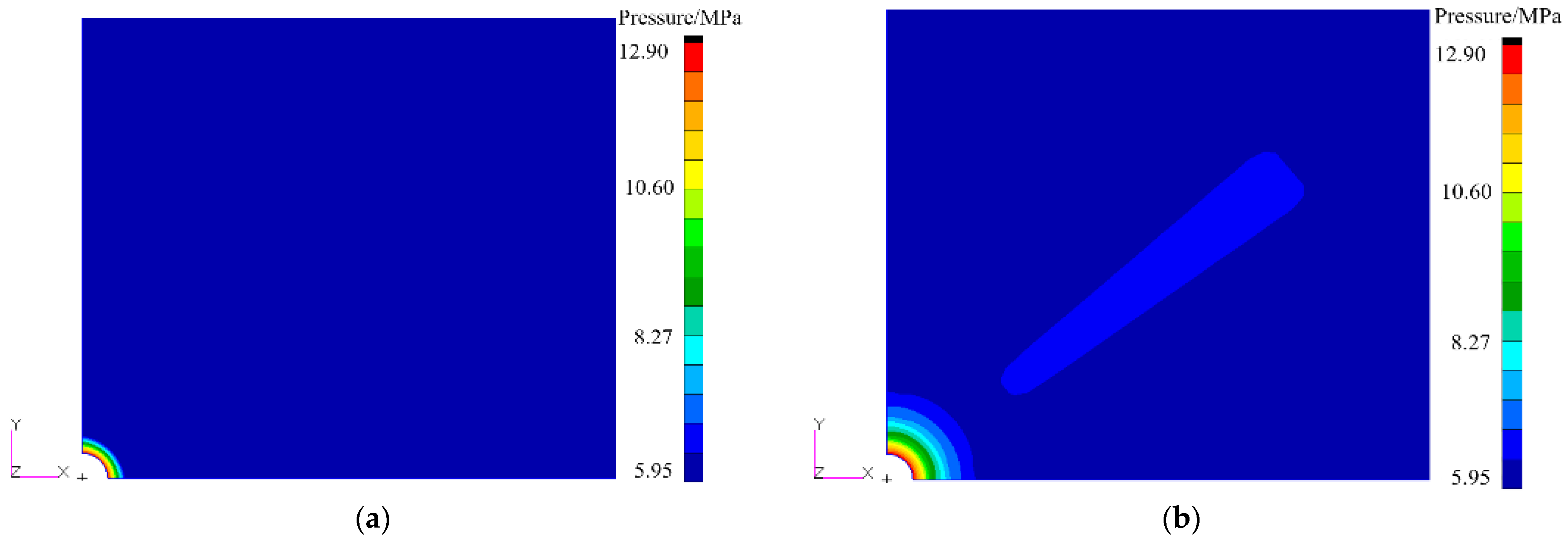
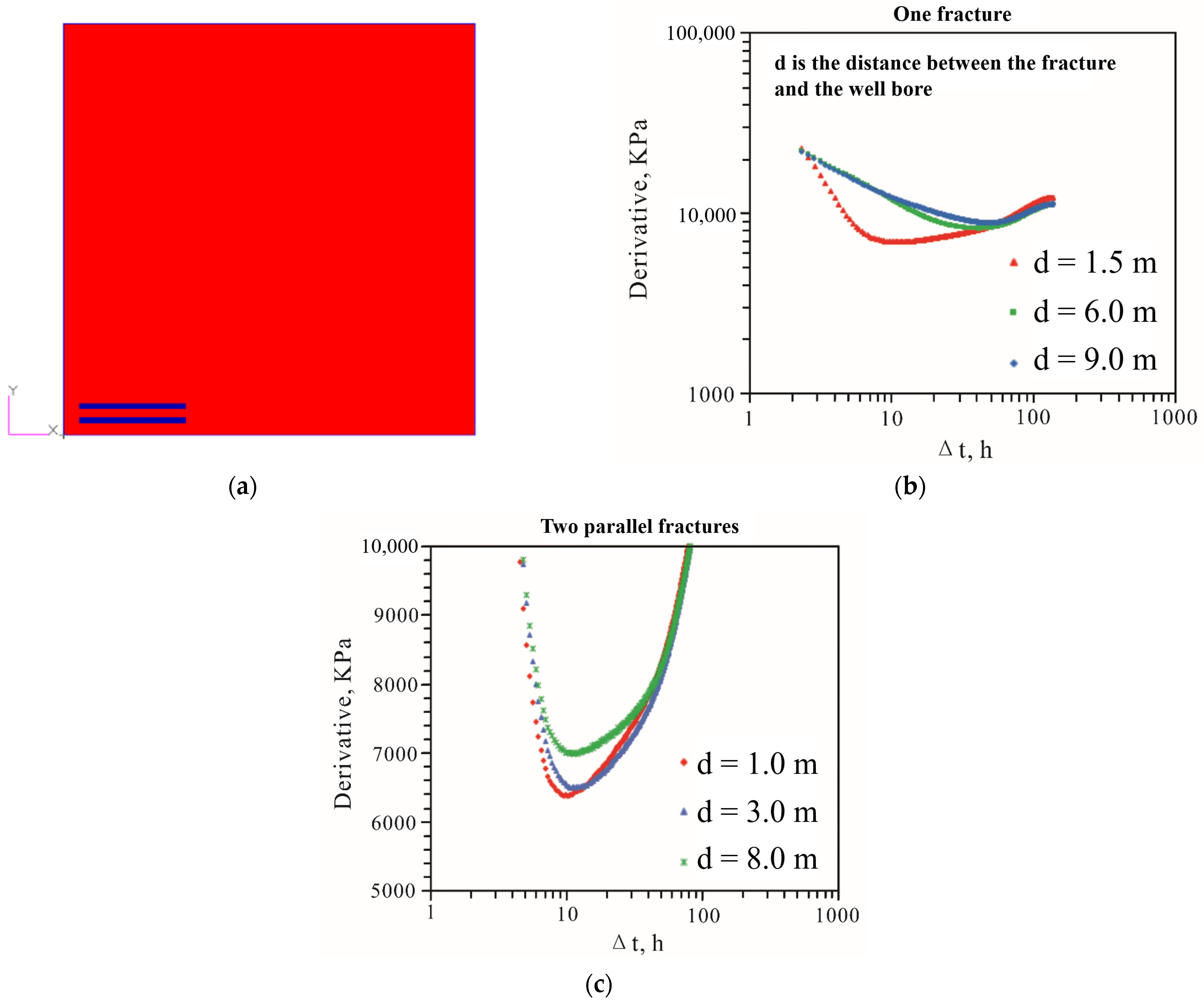
3.1.1. Effect of Relative Fracture Location on the Test Well

Whether or not the fractures intersect the wellbore has a significant impact on pressure transient behaviors. In some wells, wellbores are intersected by fractures. However, most natural fractures are located near the wellbore but do not intersect the wellbore. The propagation process of the pressure gradient near the wellbore during water injection and the variation of bottom-hole pressure with shut-in time were studied. When the wellbore was intersected by a fracture, the pressure gradient propagated with the water injection. The fluid quickly filled the fracture (Figure 4a). Then, the fracture linear flow dominated the pressure transient behavior (Figure 4b). Later, the radial flow regime occurred (Figure 4c). Figure 4d shows that the longer the fracture, the larger the swept area. In other words, the longer the fracture, the higher the fluid recovery. However, when the fracture did not intersect the wellbore, the pressure propagation process was quite different. The formation’s radial flow regime was observed until the fracture was encountered (Figure 5a). Then, linear fracture flow occurred (Figure 5b) and became apparent (Figure 5c). Finally, the flow reached another radial flow regime (Figure 5d).

Figure 6 shows the pressure difference and bottom-hole pressure derivatives of the above two models after shut-in in the well. Figure 6a shows that serious fluctuation of the bottom-hole pressure occurred in the late flow period after shut-in in the well, and the equivalent formation permeability increased from the matrix permeability of 0.048 mD to 0.0855 mD due to the contribution of the fracture. Figure 6b shows that the formation permeability increased from 0.048 mD to 0.0512 mD due to the existence of the fracture near the wellbore. By comparing Figure 6a,b, it can be seen that when a small pressure difference occurred in the near-wellbore region, fluid in a fractured wellbore quickly filled the fracture and then reached a radial flow regime, but when unsteady flow occurred in the later stage of flow, the storage effect of the wellbore was significantly reduced.

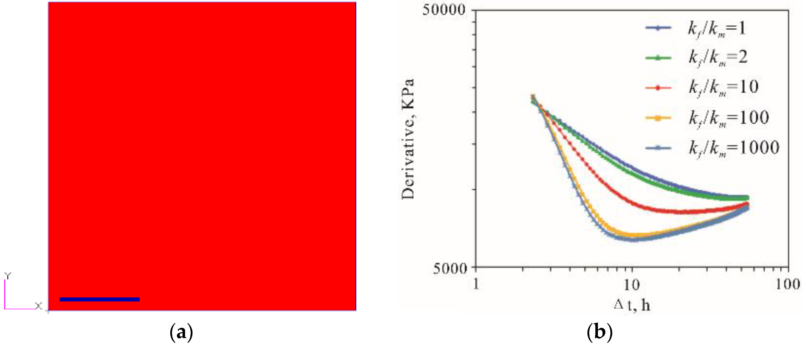
3.1.2. Effect of Fracture Permeability Relative to Matrix Permeability

Fracture permeability is one of the most significant parameters that affect the capacity of fractures to allow fluids to flow. Theoretically speaking, the higher the fracture permeability, the greater the flow capacity. However, fracture permeability is mostly limited in CSG reservoirs. Therefore, it is necessary to study the effects of fracture permeability on the flow behavior in low-permeability coal seams. A fracture was located near the wellbore (Figure 7a). The fracture half-length was 3.5 m, and the fracture width was 0.4 m. The matrix permeability was 0.048 mD, and the fracture permeabilities were 0.048 mD, 0.096 mD, 0.48 mD, 4.8 mD, and 48 mD. The ratio of the fracture permeability to the matrix permeability was denoted as k_f/k_m. The results shown in Figure 7b indicated that the derivative decreased with an increase in k_f/k_m. However, when k_f/k_m was less than 10, k_f/k_m had little effect on the derivative, and after k_f/k_m increased over 100, the derivative did not vary much. This means that when the permeability of the coal seam matrix is extremely low, a fracture with relatively high permeability cannot significantly improve the formation flow capacity, and the fracture permeability is not the main factor affecting the formation flow capacity.

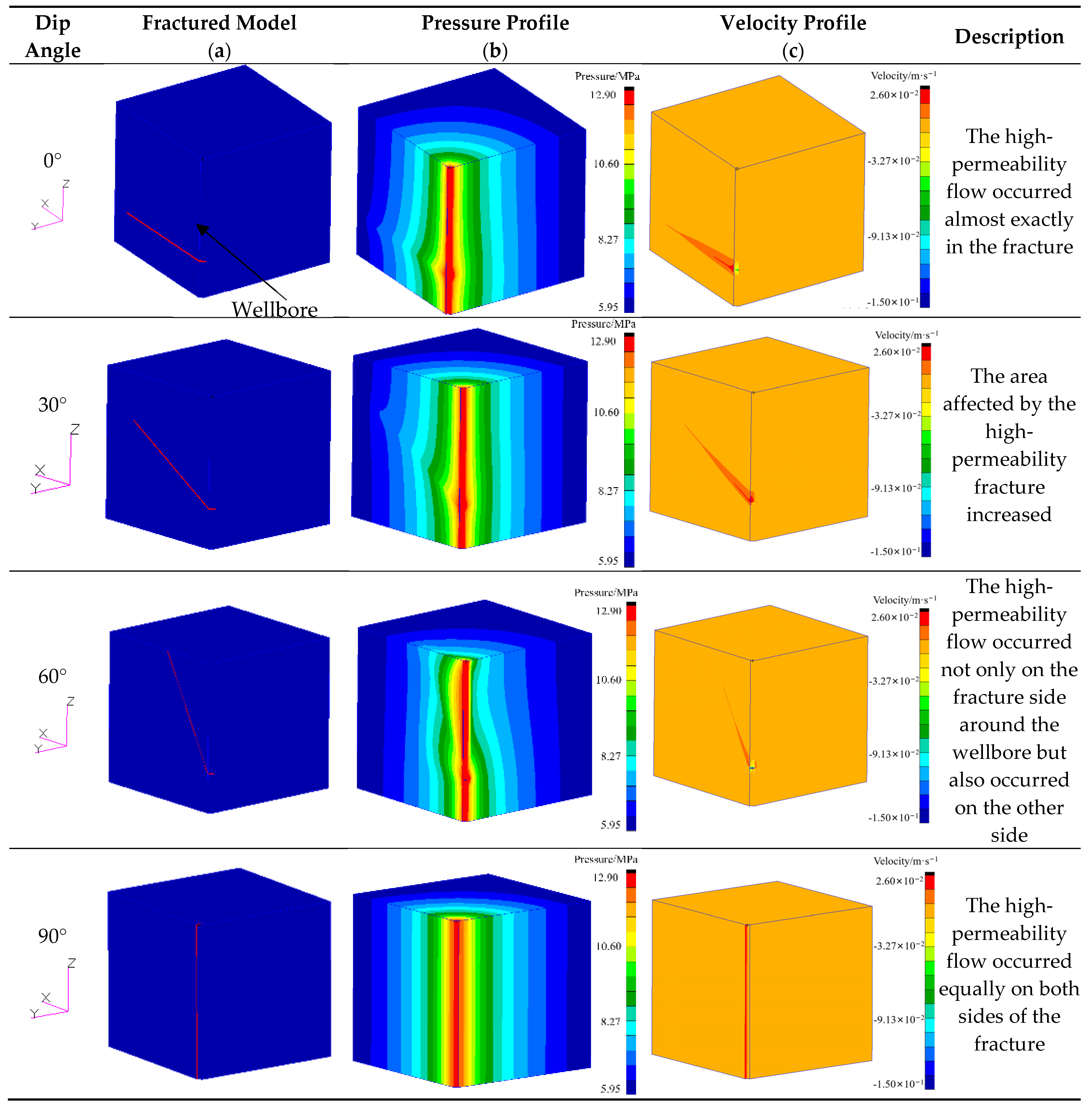
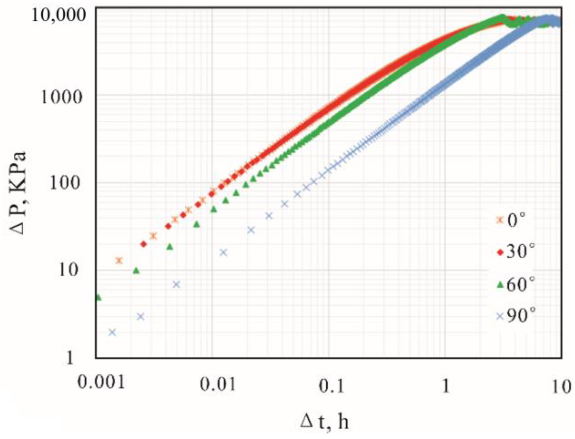
3.1.3. Effect of Fracture Dip Angles

Several inclined fracture models were built to see how pressure transient behaviors respond to these fractures. Four models contained fractures with dip angles of 0°, 30°, 60°, and 90° (Figure 8a). The fracture width was 0.4 m, and the fracture height was 0.05 m. The half-length of the fracture with a dip angle of 90° was the same as the formation thickness of 5.00 m, and the half-length of the other fractures was 5.47 m. The boundary conditions were the same as in the above models. Then, a water injection/falloff test was simulated in each model. Pressure profiles and velocity profiles were extracted to show how fractures with various dip angles affect the flow in the four models (Figure 8b,c).

Figure 8 shows that as the dip angle increased, the area affected by high-permeability fractures increased. When the fracture was perpendicular to the wellbore, the high-permeability flow occurred almost exactly in the fracture. When the dip angle was 30°, the area affected by the high-permeability fracture increased. However, when the dip angle was 60°, the high-permeability flow occurred not only on the fracture side around the wellbore but also on the other side. Additionally, when the dip angle was 90°, the high-permeability flow occurred equally on both sides of the fracture. After analyzing the bottom-hole pressure obtained from the falloff test, the relationship between pressure difference and flow time was plotted in log-log coordinates (Figure 9). Figure 9 shows the effects of fractures with different dip angles on the pressure difference in the falloff test. The early flow time greatly increased as the dip angle increased. Therefore, fractures with smaller dip angles are beneficial for fluid flow over a short period of time. However, fractures with larger dip angles are helpful in increasing the swept area and enhancing gas recovery.

3.2. Fracture Network Parametric Study

3.2.1. Effect of Fracture Spacing

Two parallel high-permeability fractures were added to the near-wellbore area in the model (Figure 10a). Figure 10b shows the effect of the fracture distance between the fracture and the wellbore. The derivative decreased as the distances decreased. In other words, when the fracture does not intersect the wellbore, the contribution of fracture permeability to formation permeability is highly dependent on the distance between the fracture and the wellbore. If a fracture is located far away from the wellbore, its contribution to the formation’s permeability is much less than that of the closer one. Then, one fracture was located 1.5 m from the wellbore, and another fracture was gradually moved farther away from the wellbore at distances of 1.00 m, 3.00 m, and 8.00 m from the fixed fracture. Figure 10c shows the effect of different fracture spacings on the derivative. It shows that fracture spacing has a significant effect on formation permeability in extremely low-permeability formations. As fracture spacing increased, the formation permeability decreased sharply.

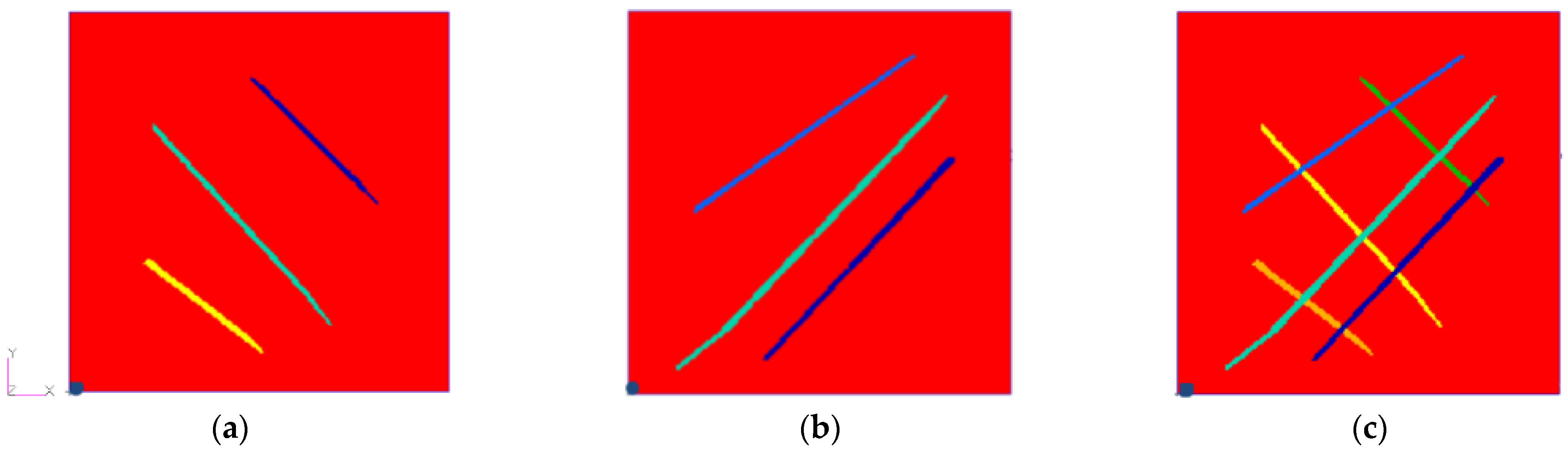
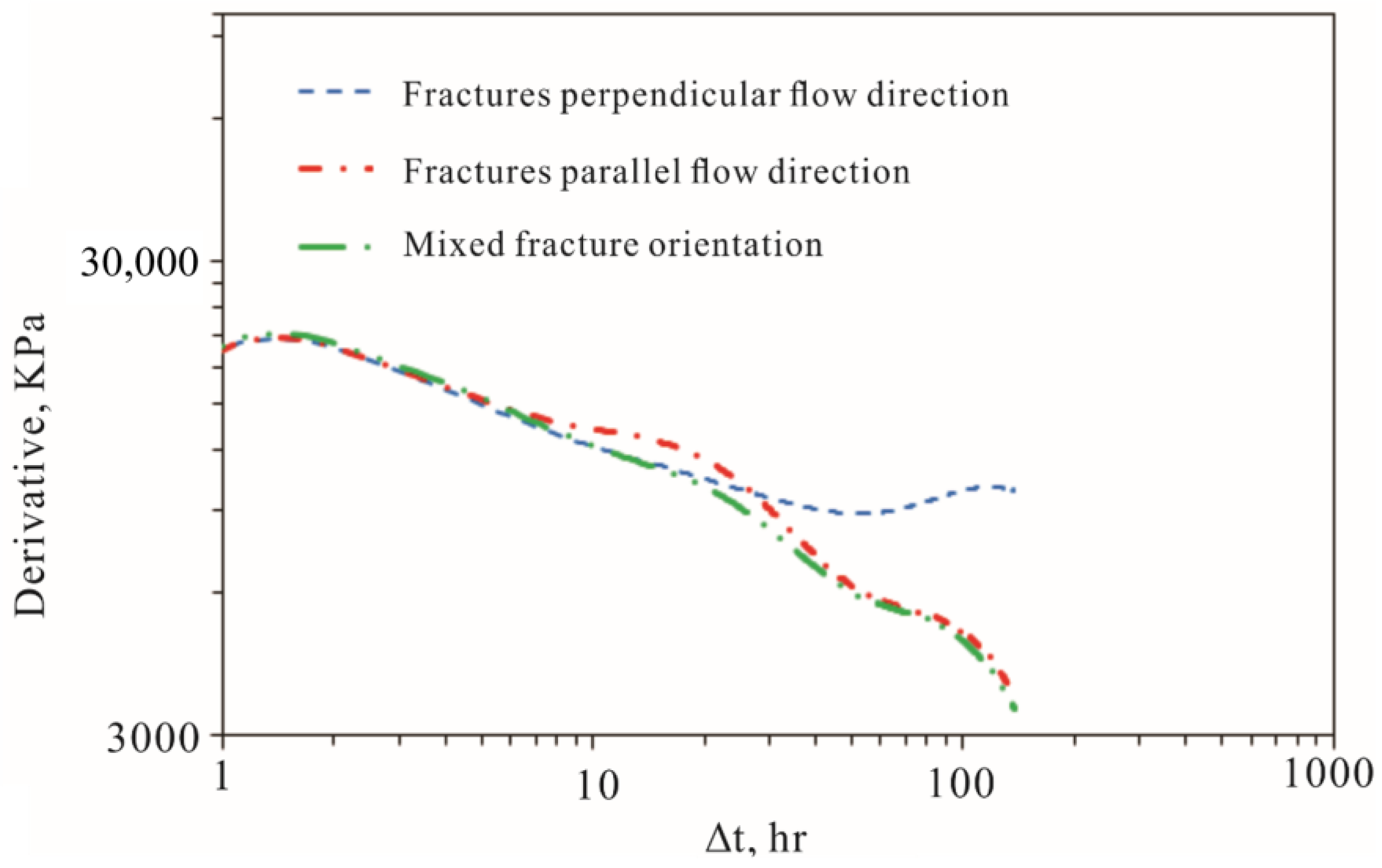
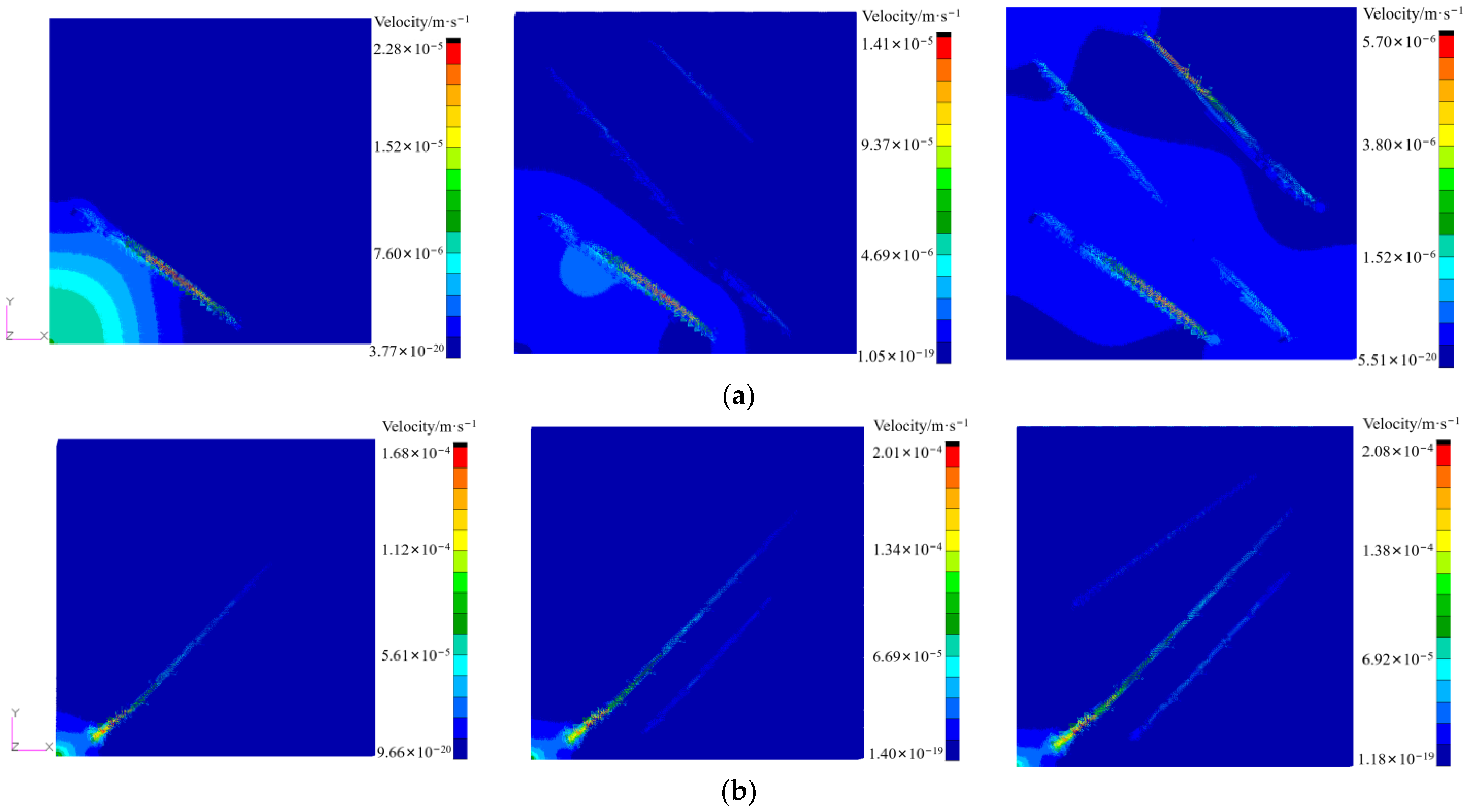
3.2.2. Effect of Fracture Network Orientation

Since fracture orientations vary widely in coal seam reservoirs at the wellbore scale, many techniques have been proposed to detect fracture orientations [51]. This section investigated numerically how different fracture orientations affect pressure transient behaviors. Different fracture orientations were set in the model (Figure 11). The fracture orientation is perpendicular to the flow direction in the formation in Figure 11a, while the fracture orientation is parallel to the flow direction in Figure 11b. Moreover, Figure 11c is the combination of the models in Figure 11a,b. Red represents the matrix in the formation; other colors represent fractures with different orientations. The blue points in the bottom left corner are the wellbores.

Figure 12 indicates that the orientation of fractures near the wellbore plays a key role in the formation’s conductivity. When the fractures were perpendicular to the flow direction, the derivative gradually decreased after the early time period and then had an upward trend. When the fracture parallel to the flow direction dominated the whole flow in the formation, the derivative of bottom-hole pressure decreased with two plateaus. This feature is usually regarded as the typical identification character of multilayers in pressure transient testing interpretation. The reason it also appears in fracture networks could be explained by analyzing the velocity profiles. As shown in Figure 13a, when the fracture orientation was perpendicular to the flow direction, the velocities in the three fractures increased sequentially along the direction of fluid diffusion, and the flow swept from the wellbore to the reservoir. In other words, the majority of the formation contributes to the whole flow. However, the flow in Figure 13b at first only occurred on the three paralleled fractures, which is quite similar to the high-permeability layers in multilayer flow. The formation velocity around fractures was almost unchanged. Therefore, two plateaus occurred in the derivative plots of both multi-layered formations and specific fractured formations.

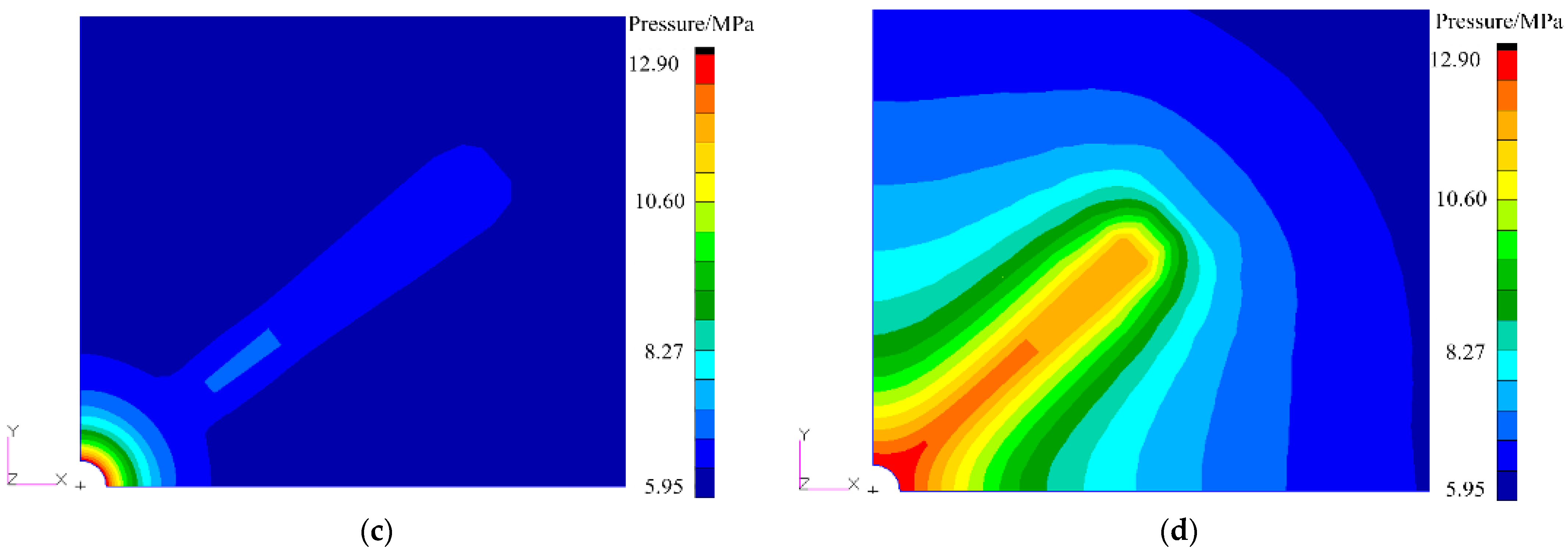
3.3. Effects of Horizontal Fracture Networks

The layers that are composed of weak minerals are easily fractured or deformed during the injection or production period, which is likely to cause high vertical heterogeneity in coal seams. The average permeability calculated for the tested multilayer, including intervals, usually overstates the expected individual single-seam outcomes [52]. This section studies the effect of the distribution of horizontal fractures (thin, high-permeability layers) on pressure transient tests. The homogeneous model was built as the reference model. The permeability was 0.048 mD. Then, the other models with horizontal fractures were built with the same average permeability as the reference model. The average permeabilities for these three heterogeneous models were calculated using the arithmetic mean method, taking the thickness weight into account [53]. The first model had two layers with thicknesses of 0.43 m and 1.47 m. Their permeabilities were 0.078 mD and 0.039 mD, respectively (Figure 14a). The second model had three layers with thicknesses of 0.77 m, 0.70 m, and 0.43 m. Their permeabilities were 0.0918 mD, 0.023 mD, and 0.0459 mD, respectively (Figure 14b). In the third model, the layer with 0.078 mD permeability in the first model was divided into eight thinner layers and distributed between the higher permeability layers (Figure 14c). The results show that the velocity in fractures increased faster, and fractures dominated the flow at the early flow time with fast-moving flow boundaries.

Figure 15 shows the derivative plots and pressure profiles of the two-layer model and the three-layer model. The pressure profiles have the same shape as the derivative in each model, which reflects the change in permeability in the vertical direction. Figure 15a shows a clear property for a two-layer model with two radial flow periods that can be identified in the derivative plot. The effective formation permeability is lower than that of the high-permeability layer but higher than that of the low-permeability layer. This is because of the interacting effect between the low-permeability layer and the high-permeability layer. Similarly, Figure 15c shows a typical feature of the three-layer model.

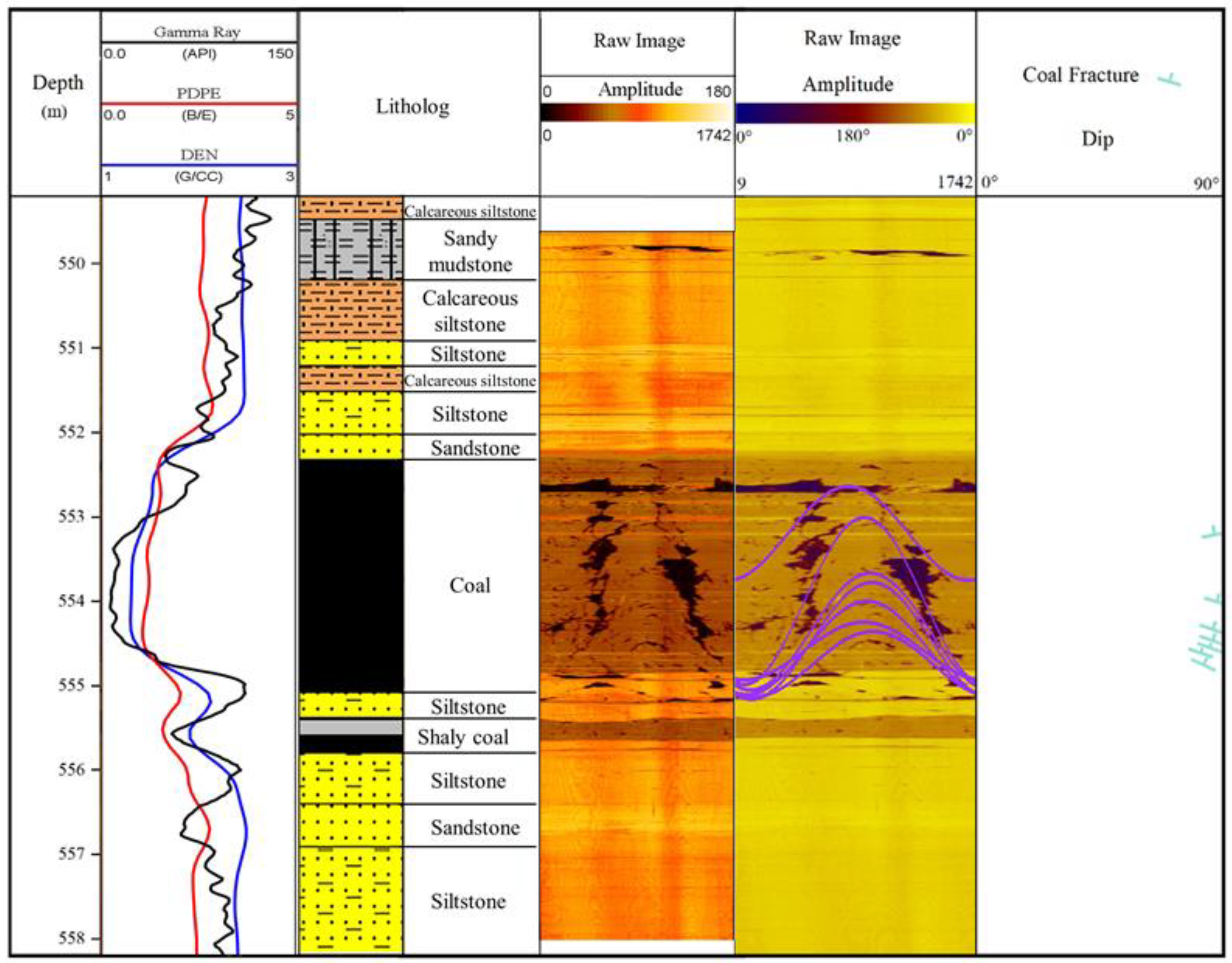
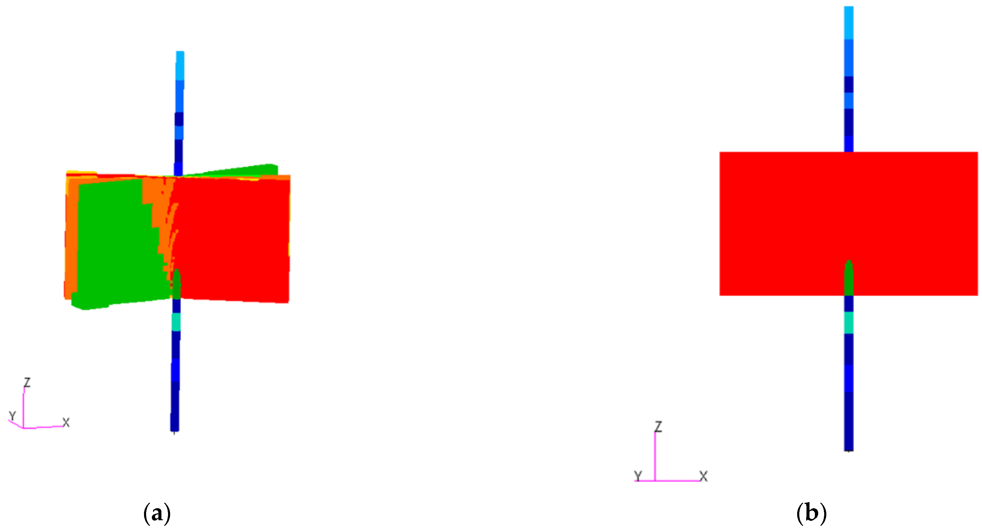
3.4. Application of the Finely Characterized Near-Wellbore Model

Conventional geological models are usually at the field scale of tens of kilometers with an extremely coarse grid that is acceptable for homogenous conventional oil and gas reservoirs. However, they may not be suitable for naturally fractured, heterogeneous, low-permeability coal seams. All the above studies have shown that both horizontal and vertical fractures have significant influences on pressure transient behaviors and how each fracture parameter affects the derivative of the pressure transient analysis. Considering the complex fracture distribution in CSG reservoirs, a finely characterized near-wellbore model was developed. In this section, a workflow based on the above research results was developed and applied to improve the accuracy of the fractured near-wellbore model of the Dalwogan 2 well. All the original static and dynamic data for the Dalwogan 2 well in this section was collected from Qdex [54].

The Dalwogan 2 well is located in the northeastern Surat Basin in southeastern Queensland. Three intervals were used in the drill stem tests (DST) at this well. This section investigated DST 1, which operated in the interval of 549.6–558 m. This interval is in the Upper Juandah Coal Measures, which belongs to the Walloon Subgroup [55]. Walloon coals typically form thin plies interbedded with claystone and siltstone beds to form thick coaly packages. Therefore, it is necessary to consider vertical heterogeneity in geological models. According to the geological description of the 549.6–558.0 m formation based on the drill stem test data (Figure 16), the tested interval is composed of 4.4 m siltstone, 0.8 m sandstone, 0.4 m shaly coal, and 2.6 m coal. Image logs can detect a large quantity of fracture information near the wellbore. According to the interpreted fractures in Figure 16, the fracture model of the actual formation thickness was built (Figure 17). The initial reservoir pressure was 5.45 MPa (Figure 18).

Table 3. Input properties of the near-wellbore model for the Dalwogan 2 well.

Parameters	Values	Units
Model radius, re	100	m
Formation thickness, h	8.3	m
Coal porosity, ϕ1	0.02
Coal permeability, k1	15.5	mD
Sandstone porosity, ϕ2	0.1
Sandstone permeability, k2	15.5	mD
Siltstone porosity, ϕ3	0.01
Siltstone permeability, k3	0.015	mD
Shaly coal porosity, ϕ4	0.02
Shaly coal permeability, k4	1.55	mD
Fracture porosity, ϕf	0.05
Fracture permeability, kf	240	mD
Initial reservoir pressure, pe	5.45	MPa

summarizes the available parameters for the Dalwogan 2 well in the Surat Basin.

After the simulated pressure buildup test in the near-wellbore model, which is the same as what has been carried out in the field, and monitoring the bottom-hole pressure, the history matching results of the measured bottom-hole pressure and simulated results for the fracture model are shown in Figure 18. The bottom-hole pressure from the pressure gauge and the fractured numerical model match very well with each other except in the middle flow time during the pressure buildup period. To show the influence of fractures on the bottom-hole pressure during the DST test, a homogeneous near-wellbore model was also built with a lower permeability of 15.5 mD. The comparison of bottom-hole pressure from the fractured model and homogeneous model is shown in Figure 19. In the early stage of pressure buildup, the bottom-hole pressure of the fractured model is greater than that of the homogeneous model. In the later stage, the gap between the two is gradually narrowed, and the pressure is approximately restored to the initial reservoir pressure. Figure 18 and Figure 19 show that a finely characterized fracture model using history matching can capture more pressure transient behaviors than the homogeneous model.

4. Conclusions

By using the in-house developed finite element software PANDAS, this paper analyzed the effect of various fracture parameters, including fracture location, the ratio of fracture permeability to matrix permeability, fracture dip angle for single fractures and fracture spacing, and fracture orientation for fracture networks, which has important guiding significance for the study of unconventional fractured reservoirs, such as carbonate reservoirs. A few conclusions are drawn as follows, based on the present research:

(1)

Fractures intersecting the wellbore can decrease the wellbore storage, but they may cause unstable flow at the late flow time when a minor pressure gradient occurs.

(2)

A longer fracture can increase formation permeability and obtain higher gas recovery because it can obtain a larger swept area in the formation than a shorter fracture. However, the increase in fracture spacing and the distance between the fracture and the wellbore significantly decrease the formation permeability in low-permeability coal seams.

(3)

The ratio of k_f/k_m equal to 100 is the optimized ratio of fracture permeability to matrix permeability in our models. In other words, the high-permeability fractures are limited in improving the formation permeability when the matrix permeability is extremely low.

(4)

The swept area when fractures are perpendicular to the flow direction is much larger than when fractures are parallel to the flow direction; however, the latter model obtains a higher formation permeability.

(5)

The fractures with smaller dip angles can allow fluids to flow more quickly to the wellbore compared to the fractures with large dip angles; however, the latter can obtain a larger affected (swept) area.

(6)

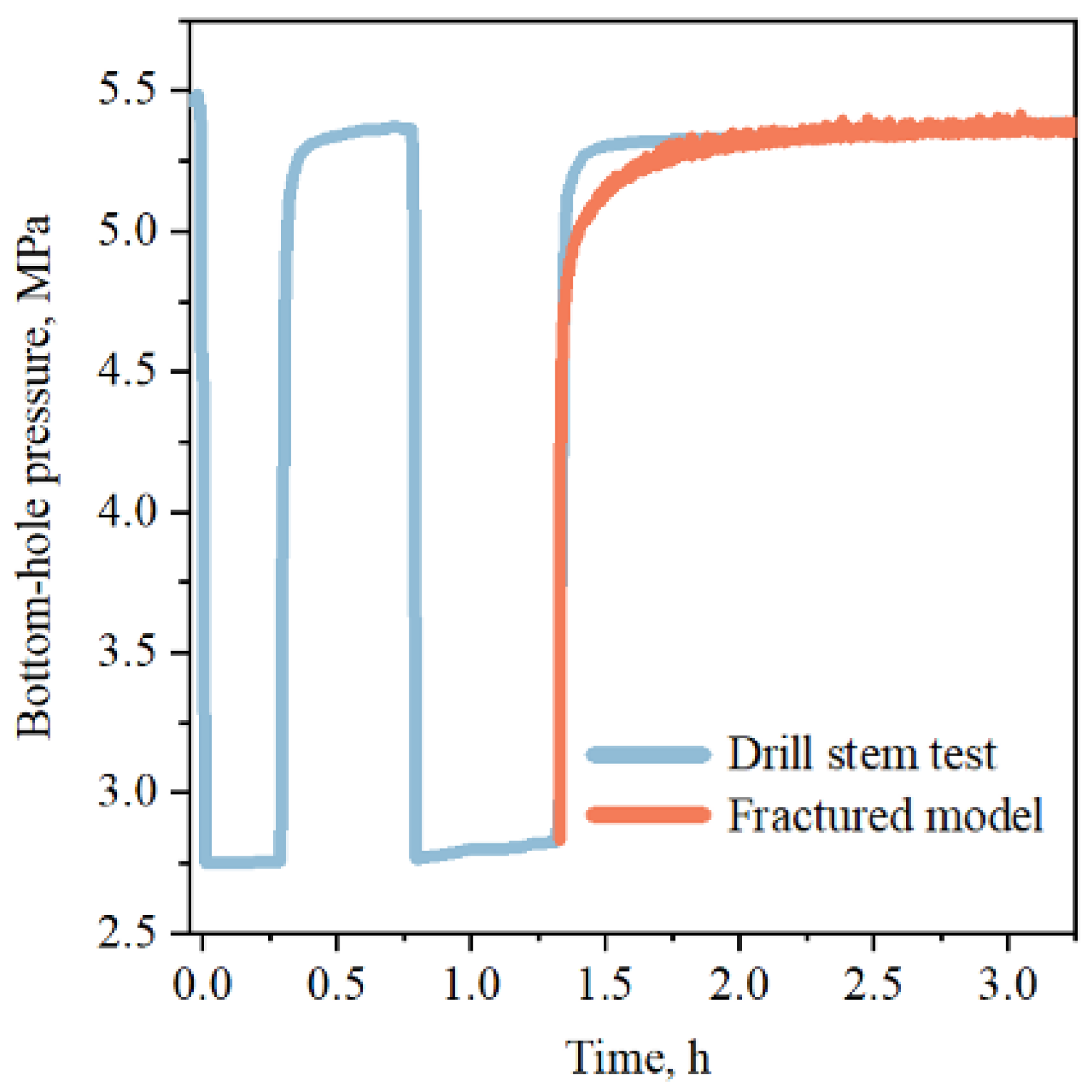
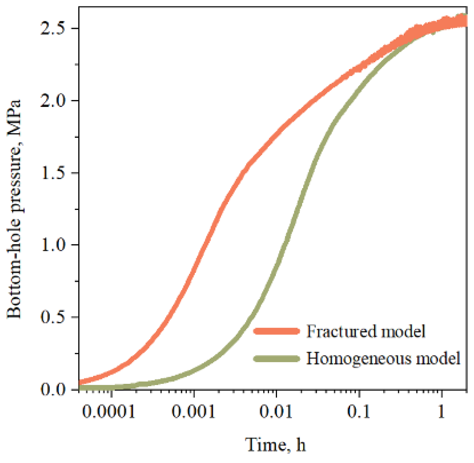
A fractured near-wellbore model is built and applied to match the history of the drill stem test in the Dalwogan 2 well in the Surat Basin. The previous parametric study results helped identify the key drivers for history matching and improved the efficiency of fracture modeling. Compared to the conventional homogeneous geological model, the bottom-hole pressure obtained from the fracture model matches very well with that measured in the field. Therefore, fractures in naturally fractured low-permeability coal seams must be accurately characterized and described in the near-wellbore model.

References

1. Ahr, W.M. Geology of carbonate reservoirs: The identification. Descr. Charact. Hydrocarb. Reserv. Carbonate Rocks 2008, 10, 269–277. [Google Scholar]
2. Xu, Z.; Li, S.; Li, B.; Chen, D.; Liu, Z.; Li, Z. A review of development methods and EOR technologies for carbonate reservoirs. Pet. Sci. 2020, 17, 990–1013. [Google Scholar] [CrossRef]
3. Zhou, Y.; Ji, Y.; Zhang, S.; Wan, L. Controls on reservoir quality of Lower Cretaceous tight sandstones in the Laiyang Sag, Jiaolai Basin, Eastern China: Integrated sedimentologic, diagenetic and microfracturing data. Mar. Pet. Geol. 2016, 76, 26–50. [Google Scholar] [CrossRef]
4. Zeng, L. Microfracturing in the Upper Triassic Sichuan Basin tight-gas sandstones: Tectonic, overpressure, and diagenetic origins. AAPG Bull. 2010, 94, 1811–1825. [Google Scholar] [CrossRef]
5. Wennberg, O.P.; Casini, G.; Jonoud, S.; Peacock, D.C. The characteristics of open fractures in carbonate reservoirs and their impact on fluid flow: A discussion. Pet. Geosci. 2016, 22, 91–104. [Google Scholar] [CrossRef]
6. Ali, J.; Ashraf, U.; Anees, A.; Peng, S.; Umar, M.U.; Vo Thanh, H.; Khan, U.; Abioui, M.; Mangi, H.N.; Ali, M.; et al. Hydrocarbon potential assessment of carbonate-bearing sediments in a Meyal Oil Field, Pakistan: Insights from logging data using machine learning and quanti elan modeling. ACS Omega 2022, 7, 39375–39395. [Google Scholar] [CrossRef]
7. Delavar, M.R. Hybrid machine learning approaches for classification and detection of fractures in carbonate reservoir. J. Pet. Sci. Eng. 2022, 208, 109327. [Google Scholar] [CrossRef]
8. Otchere, D.A.; Ganat, T.O.A.; Gholami, R.; Ridha, S. Application of supervised machine learning paradigms in the prediction of petroleum reservoir properties: Comparative analysis of ANN and SVM models. J. Pet. Sci. Eng. 2021, 200, 108182. [Google Scholar] [CrossRef]
9. Chen, H.; Yin, X.; Gao, C.; Zhang, G.; Chen, J. AVAZ inversion for fluid factor based on fracture anisotropic rock physics theory. Chin. J. Geophys. 2014, 57, 968–978. [Google Scholar]
10. Zong, Z.; Sun, Q.; Li, C.; Yin, X. Young’s modulus variation with azimuth for fracture-orientation estimation. Interpretation 2018, 6, T809–T818. [Google Scholar] [CrossRef]
11. Craft, K.L.; Mallick, S.; Meister, L.J.; Van Dok, R. Azimuthal anisotropy analysis from P-wave seismic traveltime data. In SEG Technical Program Expanded Abstracts 1997; Society of Exploration Geophysicists: Dallas, TX, USA, 2–7 November 1997; pp. 1214–1217. [Google Scholar]
12. Al Dulaijan, K.; Margrave, G. VVAZ Analysis for Seismic Anisotropy in the Altamont-Bluebell Field. In Proceedings of the 2016 SEG International Exposition and Annual Meeting, Dallas, TX, USA, 16–21 October 2016. [Google Scholar]
13. Ashraf, U.; Zhang, H.; Anees, A.; Nasir Mangi, H.; Ali, M.; Ullah, Z.; Zhang, X. Application of unconventional seismic attributes and unsupervised machine learning for the identification of fault and fracture network. Appl. Sci. 2020, 10, 3864. [Google Scholar] [CrossRef]
14. Jiang, R.; Zhao, L.; Xu, A.; Ashraf, U.; Yin, J.; Song, H.; Su, N.; Du, B.; Anees, A. Sweet spots prediction through fracture genesis using multi-scale geological and geophysical data in the karst reservoirs of Cambrian Longwangmiao Carbonate Formation, Moxi-Gaoshiti area in Sichuan Basin, South China. J. Pet. Explor. Prod. Technol. 2022, 12, 1313–1328. [Google Scholar] [CrossRef]
15. Shi, H.; Luo, X.; Xu, H.; Wang, X.; Zhang, L.; Wang, Q.; Lei, Y.; Jiang, C.; Cheng, M.; Ma, S. Identification and distribution of fractures in the Zhangjiatan shale of the Mesozoic Yanchang Formation in Ordos Basin. Interpretation 2017, 5, SF167–SF176. [Google Scholar] [CrossRef]
16. Xue, Y.; Cheng, L.; Mou, J.; Zhao, W. A new fracture prediction method by combining genetic algorithm with neural network in low-permeability reservoirs. J. Pet. Sci. Eng. 2014, 121, 159–166. [Google Scholar] [CrossRef]
17. Matsushima, J.; Ali, M.Y.; Bouchaala, F. A novel method for separating intrinsic and scattering attenuation for zero-offset vertical seismic profiling data. Geophys. J. Int. 2017, 211, 1655–1668. [Google Scholar] [CrossRef]
18. Bouchaala, F.; Ali, M.Y.; Matsushima, J.; Bouzidi, Y.; Takougang, E.M.T.; Mohamed, A.A.; Sultan, A. Azimuthal investigation of compressional seismic-wave attenuation in a fractured reservoirSeismic wave attenuation anisotropy. Geophysics 2019, 84, B437–B446. [Google Scholar] [CrossRef]
19. Wang, H. Hydraulic fracture propagation in naturally fractured reservoirs: Complex fracture or fracture networks. J. Nat. Gas. Sci. Eng. 2019, 68, 102911. [Google Scholar] [CrossRef] [Green Version]
20. Earlougher, R.C. Advances in Well Test Analysis; Henry, L., Ed.; Doherty Memorial Fund of AIME New York: New York, NY, USA, 1977; Volume 5. [Google Scholar]
21. Economides, M.J.; Hill, A.D.; Ehlig-Economides, C.; Zhu, D. Petroleum Production Systems; Pearson Education: London, UK, 2013. [Google Scholar]
22. Warren, J.E.; Root, P.J. The behavior of naturally fractured reservoirs. Soc. Pet. Eng. J. 1963, 3, 245–255. [Google Scholar] [CrossRef] [Green Version]
23. Cinco-Ley, H. Well-test analysis for naturally fractured reservoirs. J. Pet. Technol. 1996, 48, 51–54. [Google Scholar] [CrossRef]
24. Bourdet, D. Well Test Analysis: The Use of Advanced Interpretation Models; Elsevier: Amsterdam, The Netherlands, 2002. [Google Scholar]
25. Kuchuk, F.; Biryukov, D. Transient pressure test interpretation for continuously and discretely fractured reservoirs. In Proceedings of the SPE Annual Technical Conference and Exhibition, San Antonio, TX, USA, 8–10 October 2012. [Google Scholar]
26. Agada, S.; Chen, F.; Geiger, S.; Toigulova, G.; Agar, S.; Benson, G.; Shekhar, R.; Hehmeyer, O.; Amour, F.; Mutti, M. Deciphering the fundamental controls of flow in carbonates using numerical well-testing, production optimisation, and 3D high-resolution outcrop analogues for fractured carbonate reservoirs. In Proceedings of the EAGE Annual Conference & Exhibition Incorporating SPE Europec, London, UK, 10–13 June 2013. [Google Scholar]
27. Nobakht, M.; Clarkson, C.R.; Kaviani, D. New type curves for analyzing horizontal well with multiple fractures in shale gas reservoirs. J. Nat. Gas. Sci. Eng. 2013, 10, 99–112. [Google Scholar] [CrossRef]
28. Biryukov, D.; Kuchuk, F.J. Transient pressure behavior of reservoirs with discrete conductive faults and fractures. Transp. Porous Med. 2012, 95, 239–268. [Google Scholar] [CrossRef] [Green Version]
29. Kuchuk, F.; Biryukov, D. Pressure-transient behavior of continuously and discretely fractured reservoirs. SPE Reserv. Eval. Eng. 2014, 17, 82–97. [Google Scholar] [CrossRef]
30. Deng, Q.; Nie, R.; Jia, Y.; Guo, Q.; Jiang, K.; Chen, X.; Liu, B.; Dong, X. Pressure transient behavior of a fractured well in multi-region composite reservoirs. J. Pet. Sci. Eng. 2017, 158, 535–553. [Google Scholar] [CrossRef]
31. Chen, Z.; Liao, X.; Sepehrnoori, K.; Yu, W. A semianalytical model for pressure-transient analysis of fractured wells in unconventional plays with arbitrarily distributed discrete fractures. SPE J. 2018, 23, 2041–2059. [Google Scholar] [CrossRef]
32. Liu, H.; Zhao, X.; Tang, X.; Peng, B.; Zou, J.; Zhang, X. A Discrete fracture-matrix model for pressure transient analysis in multistage fractured horizontal wells with discretely distributed natural fractures. J. Pet. Sci. Eng. 2020, 192, 107275. [Google Scholar] [CrossRef]
33. Liu, X.; Li, D.; Yang, J.; Zha, W.; Zhou, Z.; Gao, L.; Han, J. Automatic well test interpretation based on convolutional neural network for infinite reservoir. J. Pet. Sci. Eng. 2020, 195, 107618. [Google Scholar] [CrossRef]
34. Najurieta, H.L. A theory for pressure transient analysis in naturally fractured reservoirs. J. Pet. Technol. 1980, 32, 1241–1250. [Google Scholar] [CrossRef]
35. Jochen, V.A.; Lee, W.J.; Semmelbeck, M.E. Determining permeability in coalbed methane reservoirs. In Proceedings of the SPE Annual Technical Conference and Exhibition, New Orleans, LO, USA, 29 September–1 October 1994; pp. 203–215. [Google Scholar]
36. Meng, M.; Chen, Z.; Liao, X.; Wang, J.; Shi, L. A well-testing method for parameter evaluation of multiple fractured horizontal wells with non-uniform fractures in shale oil reservoirs. Adv. Geo-Energy Res. 2020, 4, 187–198. [Google Scholar] [CrossRef]
37. Liu, H.; Liao, X.; Zhao, X.; Sun, L.; Tang, X.; Zhao, L. A high-resolution numerical well-test model for pressure transient analysis of multistage fractured horizontal wells in naturally fractured reservoirs. J. Pet. Sci. Eng. 2022, 208, 109417. [Google Scholar] [CrossRef]
38. Lake, L.W.; Carroll, H.B.; Wesson, T.C. Reservoir Characterization II; Academic Press: Cambridge, MA, USA, 1991; Volume 2. [Google Scholar]
39. Xing, H.L.; Makinouchi, A. Three dimensional finite element modeling of thermomechanical frictional contact between finite deformation bodies using R-minimum strategy. Comput. Method Appl. M 2002, 191, 4193–4214. [Google Scholar] [CrossRef]
40. Xing, H.L. Numerical simulation of transient geothermal flow in extremely heterogeneous fractured porous media. J. Geochem. Explor. 2014, 144, 168–178. [Google Scholar] [CrossRef]
41. Xing, H.L.; Makinouchi, A.; Mora, P. Finite element modeling of interacting fault system. Phys. Earth Planet. Inter. 2007, 163, 106–121. [Google Scholar] [CrossRef]
42. Jin, G.; Xing, H.; Li, T.; Zhang, R.; Liu, J.; Guo, Z.; Ma, Z. An integrated approach of numerical well test for well intersecting fractures based on FMI image. Lithosphere 2022, 2021, 4421135. [Google Scholar] [CrossRef]
43. Chupin, G.; Hu, B.; Haugset, T.; Sagen, J.; Claudel, M. Integrated wellbore/reservoir model predicts flow transients in liquid-loaded gas wells. In Proceedings of the SPE Annual Technical Conference and Exhibition, Anaheim, CA, USA, 11–14 November 2007. [Google Scholar]
44. Ramey, H.J. Advances in practical well-test analysis (includes associated paper 26134). J. Pet. Technol. 1992, 44, 650–659. [Google Scholar] [CrossRef]
45. Goode, P.A.; Thambynayagam, R. Pressure drawdown and buildup analysis of horizontal wells in anisotropic media. SPE Form. Eval. 1987, 2, 683–697. [Google Scholar] [CrossRef]
46. Kamal, M.M.; Morsy, S.; Suleen, F.; Pan, Y.; Dastan, A.; Stuart, M.R.; Mire, E.; Zakariya, Z. Determination of in-situ reservoir absolute permeability under multiphase-flow conditions using transient well testing. SPE Reserv. Eval. Eng. 2019, 22, 336–350. [Google Scholar] [CrossRef]
47. Feitosa, G.S.; Chu, L.; Thompson, L.G.; Reynolds, A.C. Determination of permeability distribution from well-test pressure data. J. Pet. Technol. 1994, 46, 607–615. [Google Scholar] [CrossRef]
48. Karacan, C.Ö. Integration of vertical and in-seam horizontal well production analyses with stochastic geostatistical algorithms to estimate pre-mining methane drainage efficiency from coal seams: Blue Creek seam, Alabama. Int. J. Coal Geol. 2013, 114, 96–113. [Google Scholar] [CrossRef] [Green Version]
49. Tao, S.; Tang, D.; Xu, H.; Gao, L.; Fang, Y. Factors controlling high-yield coalbed methane vertical wells in the Fanzhuang Block, Southern Qinshui Basin. Int. J. Coal Geol. 2014, 134, 38–45. [Google Scholar] [CrossRef]
50. Kuchuk, F.; Biryukov, D. Pressure-transient tests and flow regimes in fractured reservoirs. SPE Reserv. Eval. Eng. 2015, 18, 187–204. [Google Scholar] [CrossRef]
51. Pérez, M.A.; Gibson, R.L.; Toksöz, M.N. Detection of fracture orientation using azimuthal variation of P-wave AVO responses. Geophysics 1999, 64, 1253–1265. [Google Scholar] [CrossRef] [Green Version]
52. Burgoyne, M.W.; Clements, G.M. A probabilistic approach to predicting coalbed methane well performance using multi-seam well test data. In Proceedings of the SPE Asia Pacific Oil & Gas Conference and Exhibition, Adelaide, Australia, 14–16 October 2014. [Google Scholar]
53. Salmachi, A.; Rajabi, M.; Reynolds, P.; Yarmohammadtooski, Z.; Wainman, C. The effect of magmatic intrusions on coalbed methane reservoir characteristics: A case study from the Hoskissons coalbed, Gunnedah Basin, Australia. Int. J. Coal Geol. 2016, 165, 278–289. [Google Scholar] [CrossRef]
54. Qdex. Queensland-Geosciences Data. Available online: https://geoscience.data.qld.gov.au/data/borehole/bh060813 (accessed on 13 December 2021).
55. Jones, G.D.; Patrick, R.B. Stratigraphy and coal exploration geology of the northeastern Surat Basin. Coal Geol. 1981, 1, 153–163. [Google Scholar]
Figure 1. (a) Pressure distribution at t = 6.5 h; (b) Velocity distribution at t = 6.5 h.
Energies 16 02505 g001
Figure 2. Comparison of semilog plots of bottom-hole pressure during the pressure drawdown test calculated by PANDAS and Eclipse.
Energies 16 02505 g002
Figure 3. (a) The near-wellbore model scheme; (b) A quarter of the near-wellbore model with constant pressure and flow rate (top view); (c) Magnification of the black block in (a); (d) A heterogeneous coal package (cross-section).
Energies 16 02505 g003aEnergies 16 02505 g003b
Figure 4. (ad) Pressure propagation during water injection in the model when a fracture intersects the wellbore (top view), MPa.
Energies 16 02505 g004
Figure 5. (ad) Pressure propagation during water injection in the model when the fracture does not intersect the wellbore (top view), MPa.
Energies 16 02505 g005aEnergies 16 02505 g005b
Figure 6. Log-log plot of the pressure difference and derivative of bottom-hole pressure. (a) A fracture intersecting the wellbore; (b) A fracture near the wellbore.
Energies 16 02505 g006aEnergies 16 02505 g006b
Figure 7. (a) Near-wellbore model with one fracture (blue); (b) Comparison of derivative plots with different kf/km.
Energies 16 02505 g007
Figure 8. Fracture models with different dip angles. (a) Fractures (in red) in the model; (b) A pressure profile, MPa; (c) A velocity profile at the same time during water injection, m/s.
Energies 16 02505 g008
Figure 9. Log-log plots of the pressure difference in four fracture models with different dip angles.
Energies 16 02505 g009
Figure 10. (a) Near-wellbore model with two parallel fractures; (b) A comparison of the derivative plots for models with different distances between the fracture and the wellbore; (c) A comparison of derivative plots with different distances between two parallel fractures.
Energies 16 02505 g010
Figure 11. (a) Fractures perpendicular to the flow direction; (b) Fractures parallel to the flow direction; (c) Mixed fracture orientations. The blue points represent the wellbores.
Energies 16 02505 g011
Figure 12. Comparison of the derivative plots between different fracture orientations.
Energies 16 02505 g012
Figure 13. Velocity profiles changing with water injection. (a) Fractures perpendicular to the flow direction; (b) Fractures parallel to the flow direction.
Energies 16 02505 g013
Figure 14. Velocity profiles of (a) the two-layer model, (b) the three-layer model, and (c) the multilayer model in the x-z section.
Energies 16 02505 g014aEnergies 16 02505 g014b
Figure 15. (a) The derivative plot of the two-layer model; (b) The pressure profile of bottom-hole pressure for the two-layer model; (c) The derivative plot of the three-layer model; (d) The pressure profile of bottom-hole pressure for the three-layer model.
Energies 16 02505 g015aEnergies 16 02505 g015b
Figure 16. The well log of Dalwogan 2. Log interpretation shows that there are seven open fractures in the interval 548.5–558.5 m.
Energies 16 02505 g016
Figure 17. (a) Partial fracture networks near the wellbore area; (b) Partial single fracture near the wellbore area.
Energies 16 02505 g017
Figure 18. Comparison of the bottom-hole pressure from the gauge and the fractured model.
Energies 16 02505 g018
Figure 19. Comparison of the bottom-hole pressure from the fractured model and homogeneous model.
Energies 16 02505 g019