The Maximum Power Point Tracking (MPPT) of a Partially Shaded PV Array for Optimization Using the Antlion Algorithm

Abstract

The antlion optimizer (ALO) algorithm is used in this article for maximum power point tracking (MPPT) of a solar array. The solar array consists of a single module, while there are 20 cells in the module. The voltage and current ratings of each cell are 2 V and 2.5 A, making a 100 W array in ideal condition. However, the voltage and current characteristics of the PV cell are unable to achieve maximum power. Therefore, the ALO was used for MPPT. The results of the ALO are compared with the traditional metaheuristic approaches, perturb and observe ($P\&O$) and flower pollination (FP) algorithms. Comparison of the ALO with the stated algorithms is conducted for two cases: when solar irradiance is 1000 W/m${}^2$ and when it drops to 200 W/m${}^2$ at first then reaches 1000 W/m${}^2$. The change of irradiance is performed to simulate the partial shading condition. The simulation results depict that maximum power for the first case using the ALO reaches 91.3 W in just 0.05 s, while the $P\&O$ and PFA reach 90 W after 0.64 and 2 s, respectively. For the case of partial shading, maximum power using the ALO drops to 55 W when irradiance decreases to 200 W/m${}^2$ and then increases with the increase in irradiance reaching 91.3 W which clearly shows that the ALO outperforms the P&O and FPA.

1. Introduction

The maximum power point tracking problem of a solar power generation system was solved using a biologically inspired metaheuristic and an antlion optimisation algorithm. The proposed method is evaluated for no shading and partial shading. The case of partial shading is simulated by reducing the irradiance value over time. Simulation results depict that the ALO tracks maximum power (MP) whether the environment conditions are normal or adverse. Results of the antlion optimizer (ALO) are compared with traditional and metaheuristic maximum power point tracking (MPPT) techniques, namely perturb and observe ($P\&O$) and flower pollination (FPA). The simulation results demonstrate that the ALO has better performance in terms of time taken to reach MPP. The transients of the proposed algorithms decay in $0.02$ s, while the $P\&O$ decays in 0.7 s, and the FPA transients decay in $1.4$ s. The ALO has an output power around 91 watts, whereas the existing algorithms can provide up to 90 watts. These findings increase our confidence in the performance of the ALO and demonstrate that it outperforms existing algorithms. It should be noted that the proposed method has also been tested for maximum power extraction from the photovoltaic system under partial shading conditions and compared to the $P\&O$ and FP algorithms for the same case. When shading is introduced, that is, the solar irradiance is reduced from 1000 W/m${}^2$ to 200 W/m${}^2$, the maximum power extracted from the photovoltaic system drops to 55 W and then increases after maintaining the irradiance. This research also investigates the case of a 25${}^{°}$ temperature reduction. Finally, the ALO algorithm was compared to the P&O, and FPA. It was demonstrated that the ALO has superior performance in terms of maximum power extraction compared to the others. However, there is the disadvantage of high-frequency ripples in voltage when using the ALO for MPPT in photovoltaic system.

Power extracted from the ALO has high-frequency oscillations, as can be seen in the output voltage at MPP. Although the magnitude of the oscillations is too small to damage the systems or affect the load, when the same algorithm is used to extract power in megawatts, the ripple magnitude may become too large to affect the load. Minimising voltage power ripples at MPP using the ALO can be considered a future problem to be worked on. The solar cell absorbs sunlight, causing electrons to leave their positions and form an electron-hole pair. Photons are electromagnetic energy packets found in sunlight. Photons are the fundamental constituents of electromagnetic (EM) waves.

According to Max Planck and Albert Einstein [1,2,3,4,5], EM waves have no charge or mass and only exist at energy levels. According to Planck’s findings, matter can absorb or emit light in the form of energy packets [3].

In these packets, c denotes the speed of light (3.8 × 108 ms${}^{-1}$), h denotes the Planck constant (6.626 × 10${}^{-34}$ J·s), and it denotes the wavelength of a photon. When entering the energy of the gap in the silicon band, the specific wavelength required to separate electrons from covalent bonds in the silicon material can be calculated so that they can enter the conduction band. Photons with wavelengths of 1.2 m or greater, according to [4,5,6,7,8,9], can generate electron-hole pairs in a solar cell. 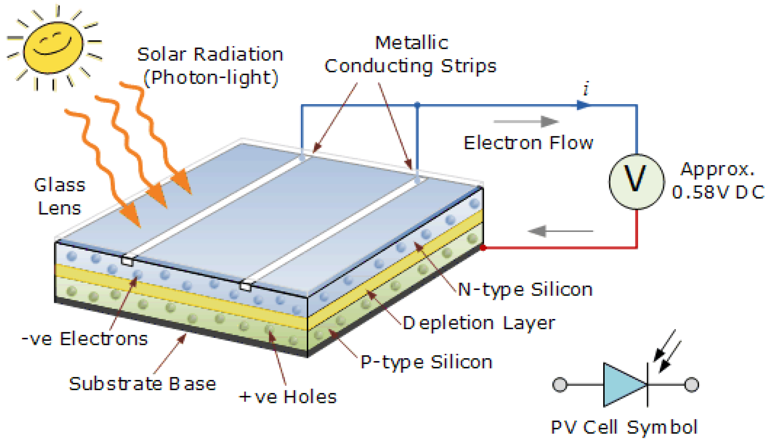When the solar cell is exposed to sunlight, it is bombarded with photons; however, only photons with a wavelength of 1.2 m or higher are absorbed by the electron of the solar cell material [10].These electrons break free of the covalent bond and form massive electron-hole pairs. Whether they are made of P-type or N-type material, electrons move to the N-type terminal and then through the external circuit to power a load before moving back to the P-type terminal and entering the solar cell. When exposed to light, a single solar cell can produce up to 0.58 volts. For voltage/current requirements, cells are connected in series/parallel to make arrays/modules. To protect the panel surface, a glass lens is mounted on top as shown in Figure 1. Solar panels can be used as a standalone source of power or in combination with micro-grids [8,9,10,11,12]. The PV system has non-linear V characteristics under variable solar irradiation and temperature conditions. In the case of a direct attached load, the power transferred from the PV system to the load is inefficient, reducing system efficiency. Researchers are working on algorithms to help extract the most power from a photovoltaic system and keep it in the best possible condition in a variety of weather conditions.

MPPT algorithms are another name for these sets of instructions. Because of this, the parts of a full photovoltaic system are the maximum power point tracking (MPPT) algorithm, a DC–DC converter, and a solar panel. In general, the MPPT algorithm should provide a fast response to sudden changes and keep track of the reference well. Most actions that are taken to achieve MPPT are based on the idea that the weather conditions will stay the same. Moving clouds, buildings that are close to photovoltaic panels, and tree shadows can all cause a drop in power output and a change in how the system works. It is possible for partial shading to cause multiple power peaks. The conventional MPPT design cannot achieve either global or local peak power. When there is some partial shading, the traditional MPP cannot keep up with the global peak power. Instead, it moves toward the local peak power. This occurs because the global peak is lower than the local peak. The focus of some current research is on making a new MPPT algorithm for a photovoltaic system. The goal is for the system to work well in a wide range of weather conditions. Several test-case scenarios, such as full irradiance, partial shading, full shading, and so on, are created in order to validate the work that has been conducted. For the purpose of running all of the test cases, a simulation environment is developed in MATLAB Simulink. The proposed algorithm is compared to other MPPT algorithms that are considered state of the art to see how well it works.

2. Literature Review

The MPP of a photovoltaic module varies with temperature and radiance level, making optimal matching difficult at all radiation levels. Most researchers have focused on adjusting the power supply of the DC–DC converter, which serves as a connecting module between PV call and load, in order to extract the most power from the module. The duty cycle of the converter is varied to obtain MP such that the load requirements are fulfilled. Many MPPT algorithms have been proposed with varying degrees of effectiveness, cost, and complexity as a result of the number of sensors used, processor requirements, and hardware implementation [13].

Incremental inductance, neural network control (NNC), P&O, hill climbing, current sweep, ripple correlation control, load current or voltage maximization, fractional open circuit voltage and short circuit current, fuzzy logic, and DC link capacitor drop control are a few examples [14,15,16,17,18]. Over time, numerous researchers have proposed a variety of new ideas for MPPT that function better. If the open circuit voltage is represented by $V_0$ and the panel voltage in MPP by $V_p$, then the algorithm proposition can be shown in Equation (1).

$$\frac{V_0}{V_p}-D\le 1$$

(1)

where D denotes the converter duty cycle. The hill climbing principle underlies the $P\&O$ MPPT methodology, which periodically increases or decreases the panel’s terminal current or voltage while comparing the current power output to the previous one. A small voltage perturbation is introduced into the specific working voltage of the solar panel by recording a change in current in the direction of power [19]. The algorithm’s sole operating principle is that as the current power output increases, so does the voltage perturbation; however, the voltage perturbation is in a different direction than the current. One of the main limitations of the algorithm is that at the constant perturbation step, oscillations occur near MPPT which disturb the system’s permanence and decrease power generation efficiency [20,21].

Furthermore, the modified algorithms work in the presence of limited partial shading. In the event of unpredictable environmental conditions, these modified methods will not be able to track the MPP. To improve the reliability and performance of solar power systems, many MPPT control methods based on artificial intelligence (AI) and soft computing methodologies have been proposed. AI-based techniques are better suited to many partial shading conditions because they are more reliable, flexible, and robust. MPPT based on artificial neural networks (ANN), fuzzy logic, genetic algorithms (GA), particle swarm optimization (PSO), differential evaluation theory, cuckoo search methodology, radial movement optimization, firefly optimization technique, gray wolf optimization, and ant colony optimization (ACO) are some of the techniques based on AI and soft computing that are currently available in the literature.

Only a few articles in the literature design ACO for MPPT control under specific shading circumstances and assess the performance of ACO [22]. The ACO approach is effective under various shading situations and may discover a global MPPT. The voltage of a PV array is used to represent each location for ACO. Additionally, the panel’s power output is chosen as an objective function. The optimization problem is constrained by the environmental factors, which include different shading patterns. Since only one current sensor is needed, the ACO method can attain the global maximum faster than other algorithms and can be implemented with less hardware.

ACO, unlike PSO, is not affected by the initial condition. ACO has been combined with other optimization algorithms in a few more studies, such as [23], where ACO is used to optimize the parameters of an adaptive FL controller for MPPT control. The hybrid approach reduced steady-state inaccuracy while enhancing dynamic response. The ant adaptive FL MPPT control is presented in [24], and the ACO design method is utilised to determine how the gains from the fuzzy logic controller would be calculated. Pollination aids in the generational evolution of plants. Abiotic and biotic pollination are also possible. Pollen from the same species of flowers is transported to others during abiotic pollination, which is caused by air, whereas pollen from different species may be transferred during biotic pollination, which is mostly caused by honeybees, birds, and bats. Some 90% of pollination in the FPA occurs through cross-pollination, and the remaining 10% is self-controlled and described with the help of a probability function. 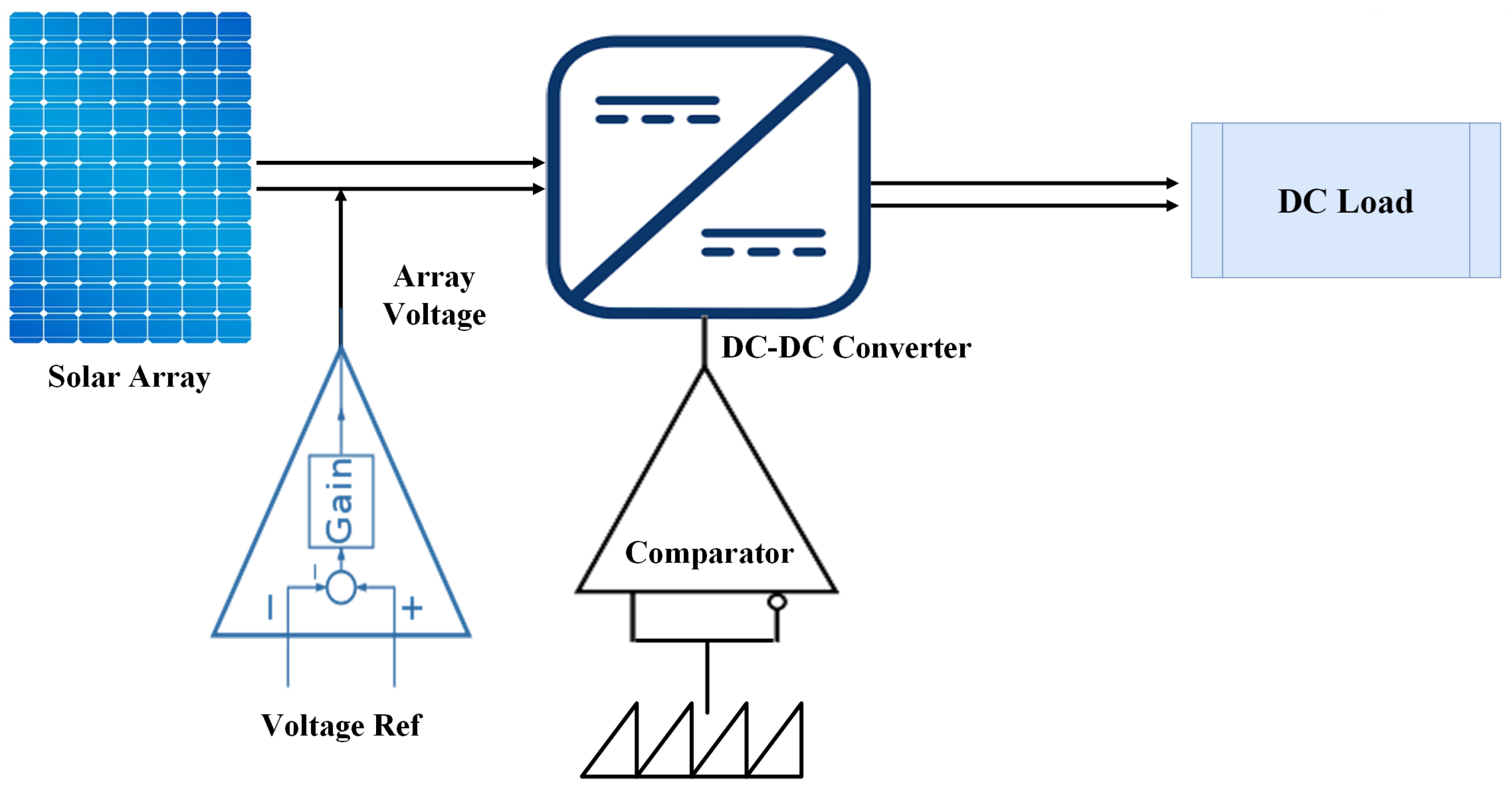Figure 2 illustrates the application of the FPA method for MPPT first. According to the literature that is currently available, the FPA algorithm performs well in partial shading settings and can achieve MPPT when there are multiple peaks. This is supported by the full flowchart that includes the approach of the FPA method for MPPT. A modified FPA is presented in [25] for MPPT.

This technique corrects the flaw in which the FPA readily reaches the local maximum and converges gradually by affecting the transition between dual-mode optimization by both the switching probability and the population’s fitness values.

Despite their simplicity in implementation, fast convergence to local optimum, and minimal hardware requirements, traditional MPPT algorithms cannot guarantee achieving MPPT for the case of partial shading. The main reason for failure for these algorithms is that they are implemented on a hill-climbing analogy. During the iterations for forward and backward step solutions, they become stuck in the local optimum solution. For such cases, artificial intelligence (AI)-based solutions are presented for MPPT. These algorithms mimic the behavior of natural actors, i.e., birds, ants, and other animals, to make the decision making efficient for optimization. However, with the implementational complexity and cost efficiency in terms of the hardware apparatus required for validation, the choice of an MPPT algorithm is a trade-off between performance and complexity.

The learning phase of MPPT algorithms based on ANN can take several years, making it computationally demanding. Aside from that, the trained ANN can only work with the PV system it was trained for. For other solar panel systems, it will need to go through a new training process. The PSO methodology is heavily reliant on particle selection at the start, which can cause it to converge very slowly toward the global maximum. The output power is affected by adjacent structures, moving clouds, and tree shadows on the panels. Multiple power peaks occur as a result of partial shading. Traditional MPPT algorithms cannot guarantee the MPPT for a partially shaded environment.

The following are the study objectives:

• Implemention of the ALO algorithm for MPPT of a shaded photovoltaic array;
• Decrease the time taken to achieve MPPT;
• Achieve the MPPT in various shaded environments.

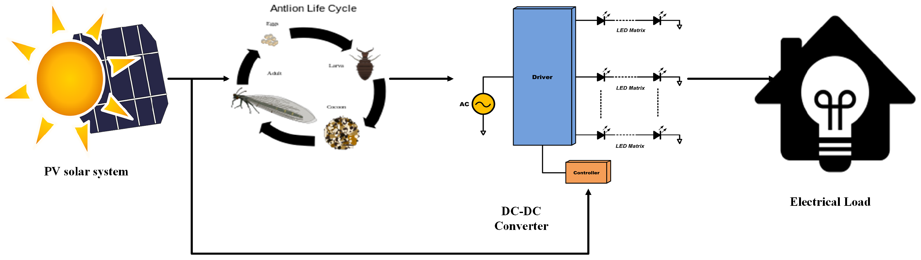
The ALO algorithm is used to achieve MPPT of a standalone photovoltaic cell. The following is a detailed discussion of the proposed methodology and algorithm for MPPT. The ALO block diagram is depicted in Figure 3.

3. System Modeling

The voltage–current (VI) curve of a PV panel and load is typically the operating point of a power generating system based on a solar panel coupled to a load or battery. The operational point and the MP supplied by the system are not necessarily the same. The solar panel array’s size must be raised in order for the battery to be fully charged during the day under conditions of average insolation. As a result, more solar panels will need to be installed, which will dramatically raise the original cost. PV-based solar-panel-based power generation systems are frequently equipped with extra gear that employs the MPPT algorithm to make up for this drawback. In order to increase the system’s efficiency in power generation, MPPT algorithms shift the operating point to a location where the module’s maximum power can be extracted.

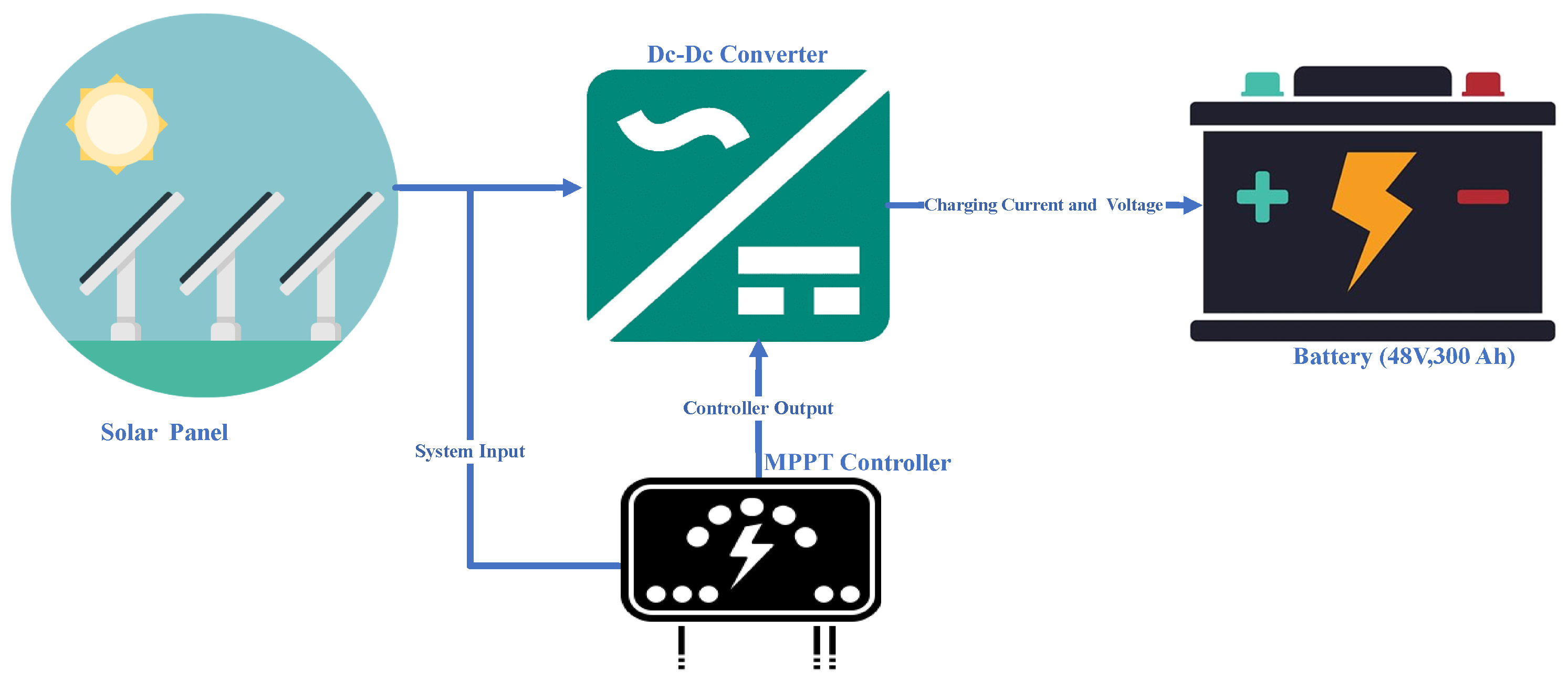
A basic circuit diagram of an MPPT-algorithm-based PV array connected to the load is presented in Figure 4. The system components include a PV array, a DC battery, a DC–DC converter, and hardware programmed with an MPPT algorithm. The MPPT algorithm operates in such a way that the duty cycle of the converter is regulated so that the PV panel operates at MPP. By using an appropriate and efficient MPPT algorithm, MPP of a PV array can be continuously achieved through controlling the duty cycle of the converter.

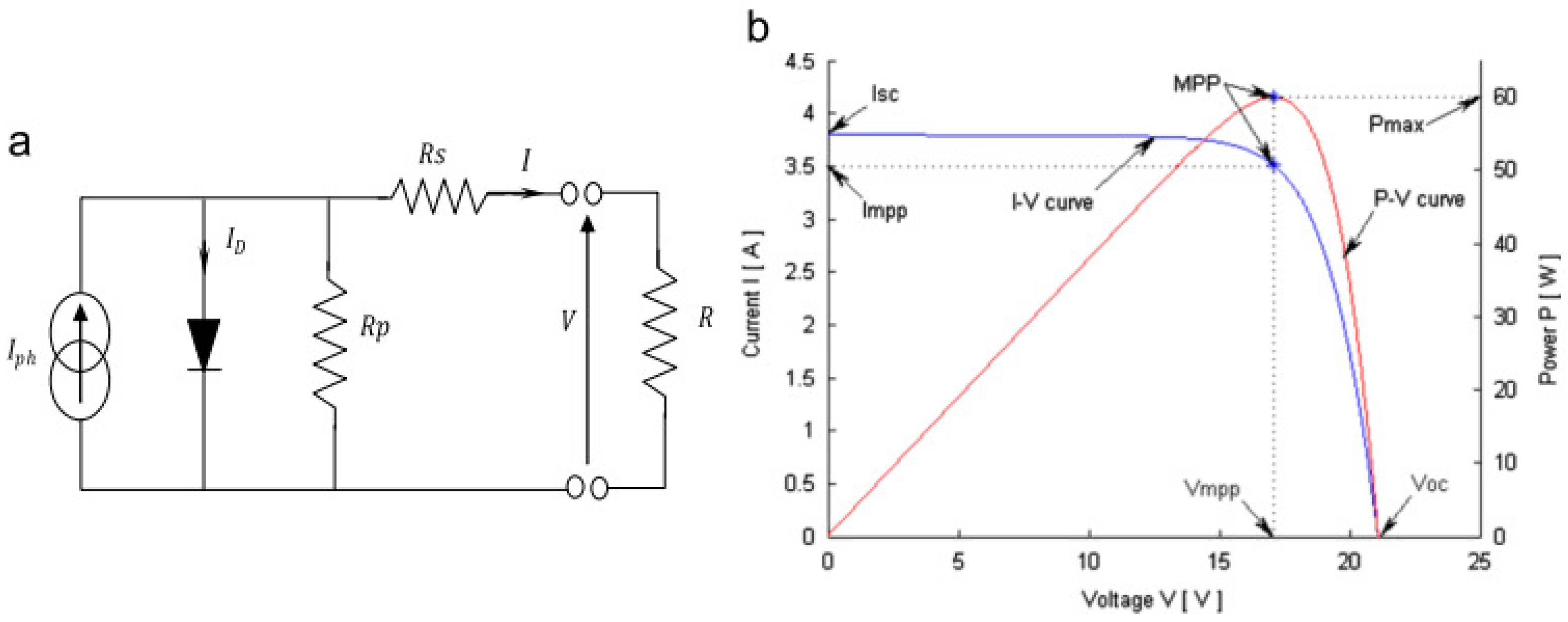
PV cells are developed by making PN junctions in thin layers of silicon; thus, their properties are comparable with those of a simple diode. A PV cell model, constructed by a diode with series resistance, is shown in Figure 5. Here, R and I denote load resistance and current available to the load, respectively. Current flowing through the diode, shunt, and resistance of the diode are denoted by $I_D$, $R_p$, and $R_s$, respectively, while $V_{th}$ denotes the voltage available at the terminals of load. The following equation can represent the current at the output of a PV cell.

$$I=I_{ph}-I_o\left[exp\left(\frac{V+I{R}_s}{a{V}_{th}}\right)-1\right]-\frac{V+I{R}_s}{R_p}$$

(2)

The diode ideality factor and reverse saturation currents are denoted by a and $I_o$, respectively. The photo-current $I_{ph}$ generated by the diode depends upon environment conditions and irradiance level. It can be given by Equation (2).

The output current of a PV array can be increased by connecting cells in parallel, while the voltage can be increased by connecting them in series. VI and PV characteristic curves of a PV cell under specific irradiance and temperature are shown in Figure 5b.

$$I_{ph}=\left[I_{scs}{T}_c+K_i\left(T-T_s{T}_c\right)\right]\frac{G}{G_s{T}_c}$$

(3)

G and I denote the normal irradiance level of the surface of a cell and short circuit current, while $G_{STC}$ and $I_{STC}$ denote the same under standard testing conditions, respectively. Standard testing temperature $T_{STC}$ is 25 ${}^{°}$C, while $K_i$ represents the short-circuit current coefficient that is provided in the system data sheet. Reverse saturation current of the diode is sensitive to the temperature and can be given by Equation (3)

$$V_{th}=\frac{K_{b}T}{q}$$

(4)

The open circuit voltage under typical test conditions is represented by $V_{o{c}_{{}_{S}TC}}$, while the open circuit voltage coefficient is $k_v$. These values can be found in the system’s data sheet, which the manufacturer provides. Equation (4) provides the diode’s terminal voltage.

$$I_o=\left(\frac{I_{scs{T}_c}+K_i\left(T-T_{s{T}_c}\right)}{\left(\frac{V_{oc}s{T}_c+K_v(T-T_{sTc})}{a{V}_{th}}\right)}-1\right)$$

(5)

where q, T, and $K_b$ denote charge on electron (1602 × ${10}^{-19}$ C ), junction temperature $\left(K\right)$, and $K_b$ and Boltzmann constant (1380 × ${10}^{-23}$ J/K).

$$I=N_p{I}_{ph}-N_p{I}_o\left[exp\left(\frac{V+1\left(\frac{N_s}{N_p}\right)R_s}{N_{s}a{V}_{th}}\right)-1\right]-\left[\frac{V+1\left(\frac{N_s}{N_p}\right)R_s}{N_{s}a{V}_{th}}\right]$$

(6)

To fulfil the power, voltage, and current demands of the load, numerous PV cells are connected in series or parallel to make a module. This is performed due to the fact that the power produced by a single sun cell is relatively little and cannot be used for practical work. A solar panel is made up of several modules that are connected together. Different manufacturers create various solar panels with varying power ratings. A group of solar panels is referred to as a solar panel array. A solar panel array can handle any current rating or voltage demand. Equations (5) and (6) provide the VI representative equation for solar cells that are organised in parallel and series, respectively.

$$V_{oc}=V_{oc},S_{STC}+K_v(T-T_s{T}_c)$$

(7)

Equation (7) demonstrates how a solar cell’s temperature affects its open-circuit voltage. As was already mentioned, temperature and irradiance fluctuations have a significant impact on solar panels. Partial shadowing conditions also have a significant impact. The irradiation levels of two connected modules in a parallel or series configuration will differ if one of the modules is shaded.

4. Methodology

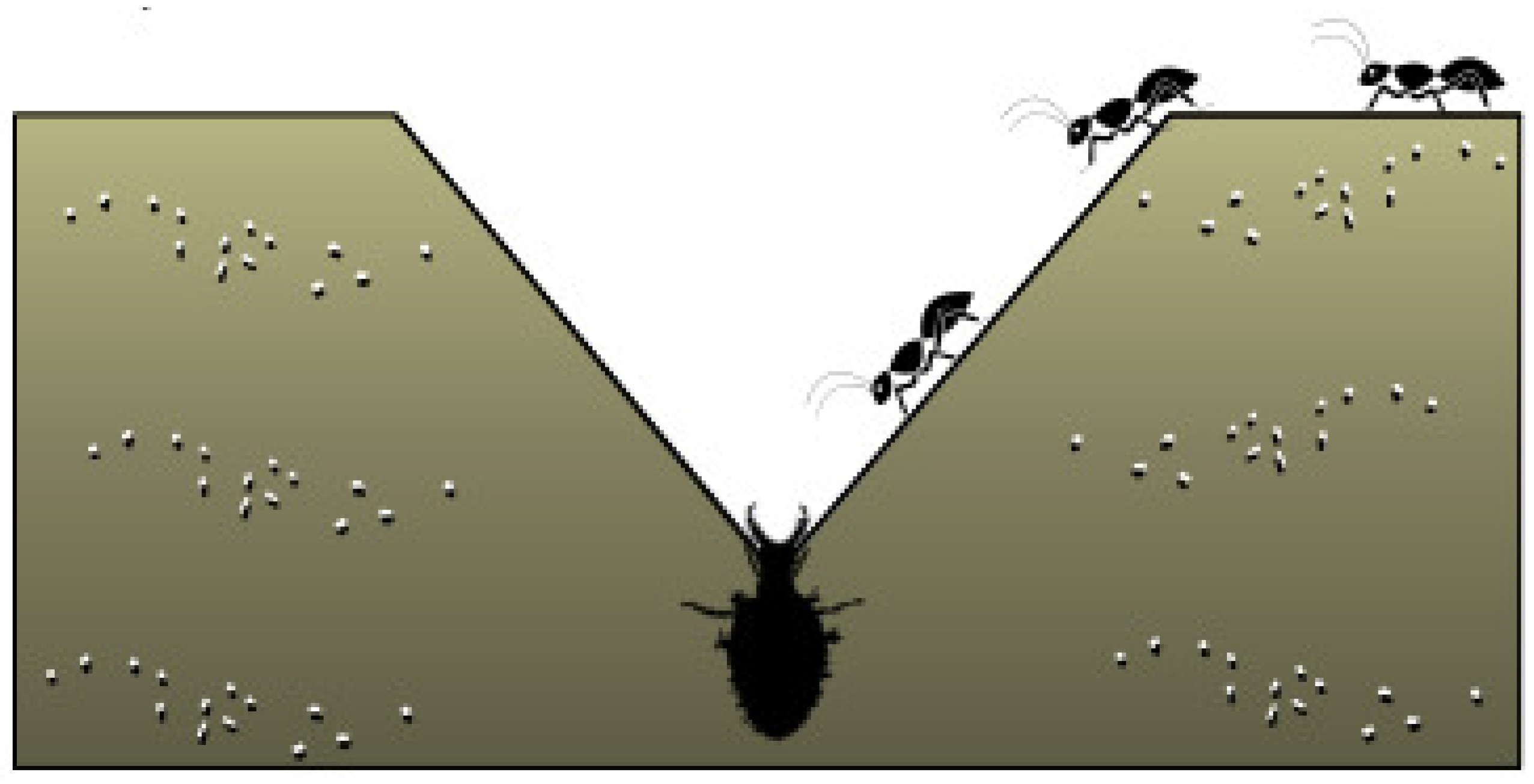
Larvae and adults are the two main phases of the antlion life cycle. The total natural life of antlions can be up to 3 years, of which 3 to 5 weeks in the life cycle are larvae and the remaining period is adults [26,27]. To become adults, antlions use a cocoon. As larvae, they hunt for ants, and in adulthood they are mainly involved in the reproduction process. Their name (antlion) is due to the unique hunting behaviour for their food, ants. With its massive jaw, an antlion digs a cone-shaped hole. The antlion hides itself at the bottom of the pit and waits for prey, preferably the ant. Hunting ants at the bottom of the pit shown in Figure 6.

Ants can simply drop to the cones’ bottoms. The antlion catches the ant after realising that it is caught in the trap. If the antlion is unsuccessful in capturing the ant, he tosses sand upward to help the ant slide into the cone’s base. When an ant is trapped in the antlion’s jaws, it is dragged underground and eaten, and the antlion prepares for his next meal. When the moon is full, the antlion burrows in larger cones to increase its hunting. By digging deeper cones, antlions boost their chances of surviving. The interaction between antlions and ants in the cones is simulated by the antlion algorithm. The antlion hunts the ants in the trap to symbolise the interaction between an ant and an antlion, whereas the ants forage in the search area. The food ant forages in a stochastic manner. It is possible to simulate the random walks of the ants/antlions as follows:

$$Z\left(s\right)=\left[0,cm\left(2r(s_1-1)\right),cm\left(2r(s_2-1)\right),cm\left(2r(s_3-1)\right),.....,cm\left(2r(s_n-1)\right)\right]$$

(8)

where $cm$, n, s,and $r\left(s\right)$ denote cumulative sum, maximum number of iterations, steps in a random walk, and stochastic function with Equation (9), respectively.

$$\left\{\begin{array}{c}1ifrng>0\hfill \\ 0ifrng\le 0\hfill \end{array}\right.$$

(9)

where $rng$ denotes a random number generated using uniform distribution in an interval of [0, 1].

$$M_{ant}=\left[\begin{array}{c}{T}_{1,1}{T}_{1,2}.....T_{1,d}\hfill \\ T_{2,1}{T}_{2,2}.....T_{2,d}\hfill \\ ............\hfill \\ T_{n,1}{T}_{n,1}.....T_{n,1}\hfill \end{array}\right]$$

(10)

where $M_{Ant}$, $T_{ij}$, n, and d denote the matrix used to store the value of the $i^{th}$ ant, dimension of the $i^{th}$ ant, total number of ants, and dimensions where an ant can move, and f denotes the objective function. The ant position refers to the specific solution of interest using the ALO. The matrices in Equation (10) provide the matrices that store the positions of the ants, the best fits, and the positions of the antlions hunting the ants (Equation (11)).

$$M_{OA}=\left[\begin{array}{c}f\left(T_{1,1}{T}_{1,2}.....T_{1,d}\right)\hfill \\ f\left(T_{2,1}{T}_{2,2}.....T_{2,d}\right)\hfill \\ ...........\hfill \\ f\left(T_{n,1}{T}_{n,1}.....T_{n,1}\right)\hfill \end{array}\right]$$

(11)

$$M_{antlion}=\left[\begin{array}{c}{N}_{1,1}{N}_{1,2}.....N_{1,d}\hfill \\ N_{2,1}{N}_{2,2}.....N_{2,d}\hfill \\ ............\hfill \\ N_{n,1}{N}_{n,1}.....N_{n,1}\hfill \end{array}\right]$$

(12)

$$M_{OAL}=\left[\begin{array}{c}f\left(N_{1,1}{N}_{1,2}.....N_{1,d}\right)\hfill \\ f\left(N_{2,1}{N}_{2,2}.....N_{2,d}\right)\hfill \\ ................\hfill \\ f\left(N_{n,1}{N}_{n,1}.....N_{n,1}\right)\hfill \end{array}\right]$$

(13)

where $M_{OAL}$ denotes the matrix used to store the antlion value, $N_{ij}$ denotes the dimension of the $i_{th}$ antlion, n represents the total number of the antlion, and f denotes the objective function. The following assumptions must be made when optimising the objective function with the ALO. Ants move randomly in search of food, that is, ants’ random movements occur in all dimensions so that the probability of finding food is maximised. 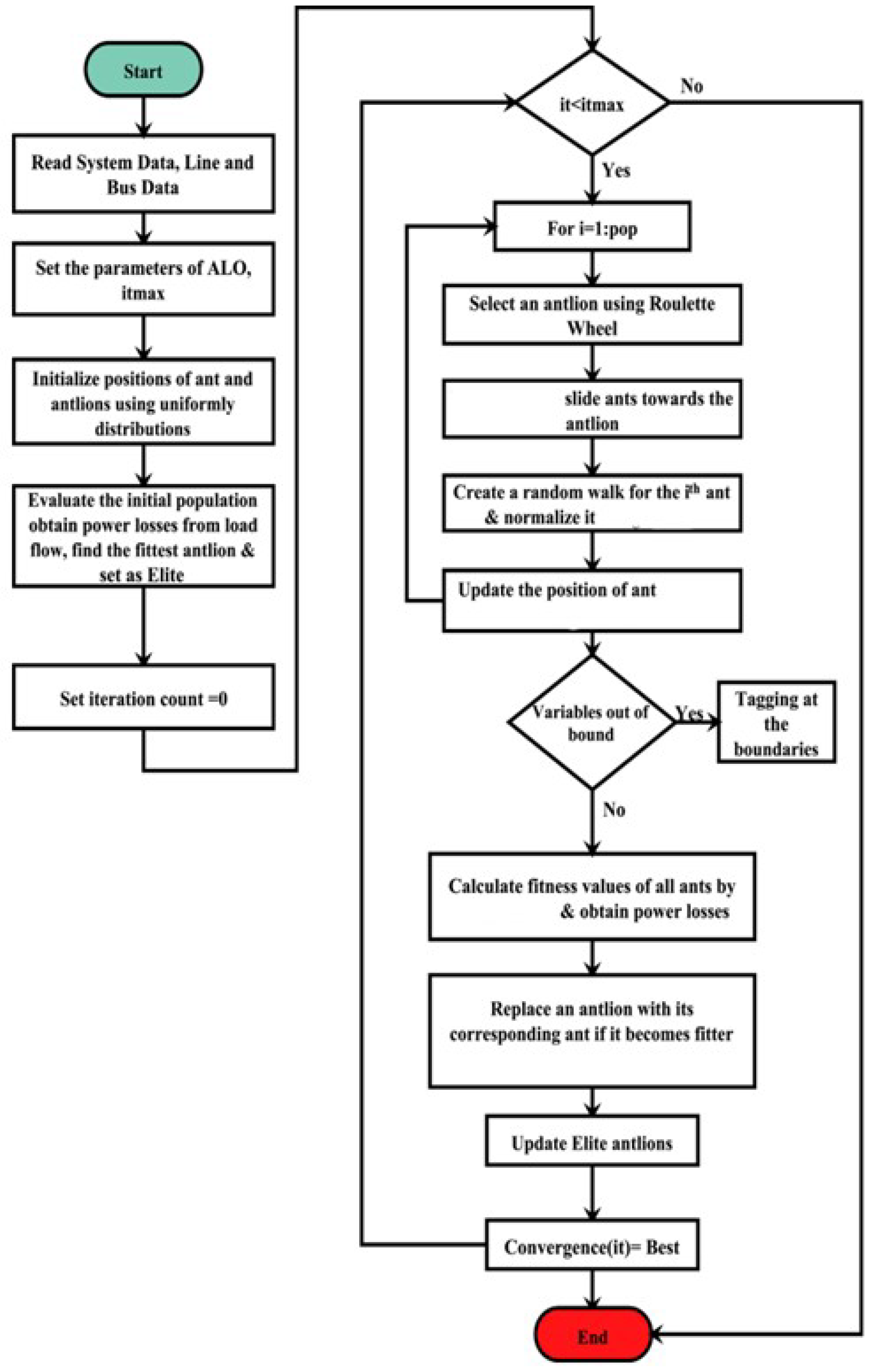Equations (12) and (13) represent ants moving randomly in the search space try to avoid the pits, which affects their random movement. Antlions, on the other hand, can construct pits in proportion to their size. Larger antlions can build larger pits and are more fit than smaller ones. Antlions that dig deeper pits have a better chance of catching their prey. Each antlion can catch every ant, and the antlion that catches an ant first is said to be the fittest. With the passage of time, the ants’ random movement towards the antlions decreases. An ant that becomes fitter in an iteration indicates that it has been captured and hunted by the antlion. After capturing an ant, the antlion repositions itself and constructs a new trap to capture another ant. The flowchart of the whole process is shown in Figure 7.

5. Simulation Results

Initially, it is assumed that the solar irradiance of 1000 W/m${}^2$ is being reached at the surface of the PV array. The environment temperature is assumed to have a constant value of 25 ${}^{°}$C. The output current and voltage of the array is 2.5 A and 40 V, respectively. Thus, the maximum available output power of the array in an ideal case is 100 W. The MPPT will have only a single curve of maximum power which can easily be tracked by any traditional MPPT algorithm. To validate the performance of the ALO, a comparative study of an ALO under the same conditions with P&O and FPA is carried out.

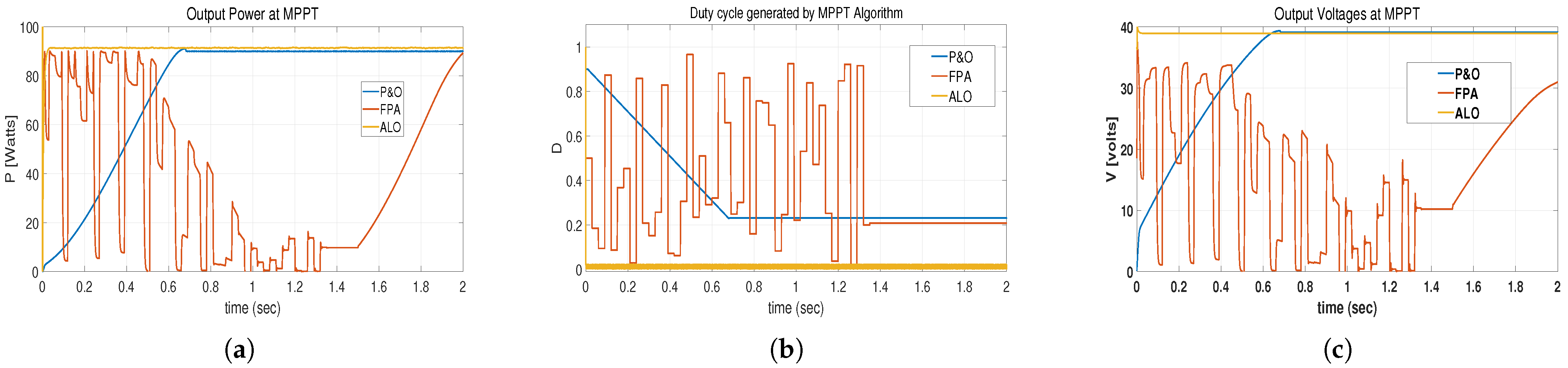
Figure 8a depicts the power output comparison of the ALO with P&O and FPA. The figure clearly shows that the MP achieved by the ALO is 91.3 W which is 1.01% increased compared to that achieved with P&O and FPA which is 90 W. In addition, the proposed approach achieves a steady value of power in 0.02 s which is much faster than the time taken by P&O (0.6 s) and FPA (1.4 s). Figure 8b,c depict the voltage and duty cycle profiles for the three algorithms. The figures clearly advocate the presence of the comparatively negligible magnitude of high-frequency oscillations using the ALO compared to that with P&O and FPA. The observations for this case are numerically presented in

Table 1. MPP, voltage, and settling time comparison.

Method	MPP	Voltage at MPP	Settling Time
	[W]	[V]	[s]
$P\&O$	90.0	39.9	0.6
$FPA$	90.0	30	1.4
$ALO$	91.3	39.4	0.02

.

The transients for the ALO decay within 0.02 s and a constant value of power and voltage is obtained while that for P&O and FPA is obtained at 0.6 and 1.4 s, respectively. The output power and voltage for the stated algorithms are shown in Figure 8, while the duty cycle comparison is presented in Figure 9.

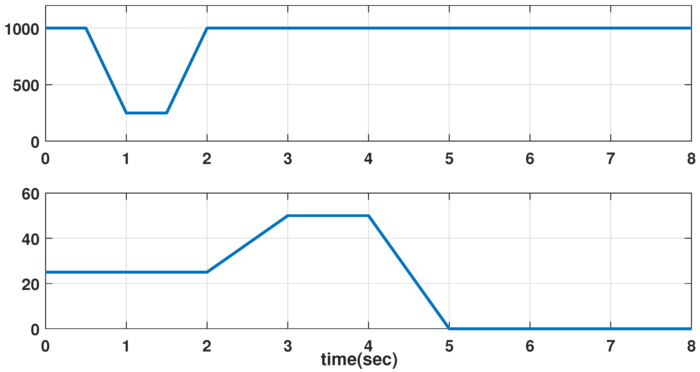
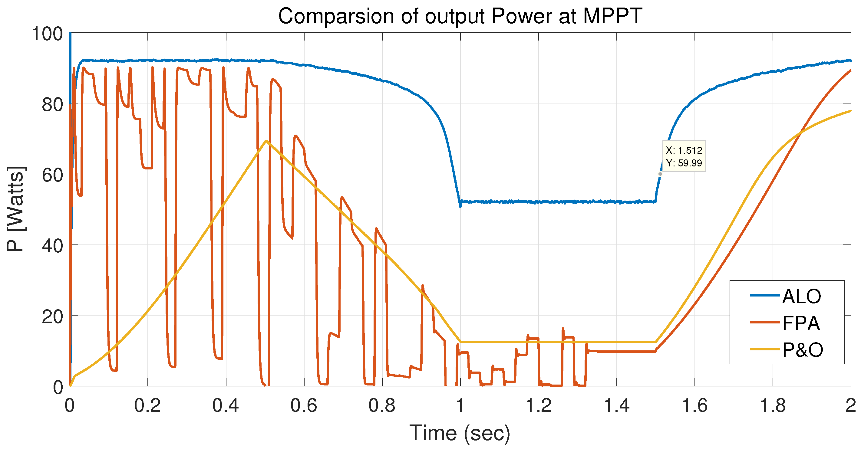
To impose partial shading in the simulation, solar irradiance is decreased 1000 W/m${}^2$ to 200 W/m${}^2$ after 0.5 s and is then increased linearly after 1.5 s until it reaches 1000 W/m${}^2$. The simulation is executed for 2 s, while a temperature change is being introduced throughout the simulation time. The output power at MPP for all the algorithms, including the ALO, is shown in Figure 10. 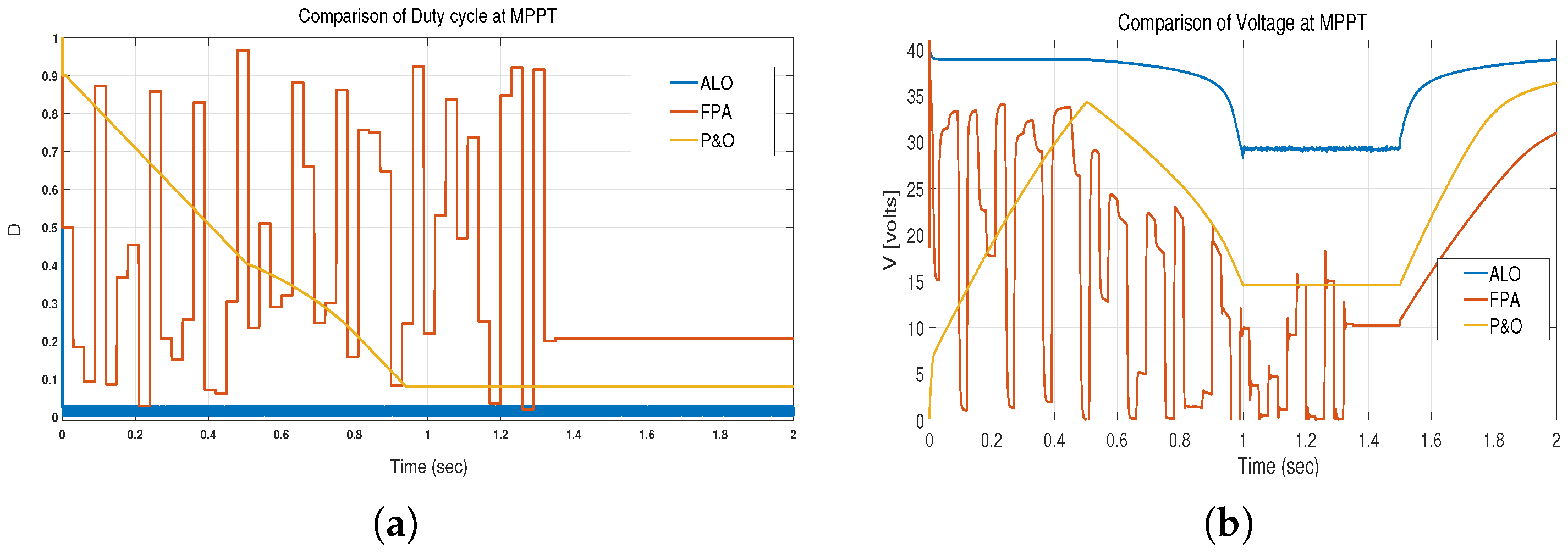As illustrated in Figure 11a,b, the power output, voltage, and duty cycle under these conditions are used to measure the performance of the ALO algorithm. According to the figure, the ALO can still produce 55 watts of power in low-irradiance situations, but as soon as the irradiance increases to normal, so does the power output. The chart also demonstrates that the output power rises and surpasses 91 watts as the temperature falls.

Figure 9 depicts the drop in voltage value from 40 to 29.5 for the case of partial shading, while it increases back to the previous value of 40 V when the irradiance level is increased. It also presents the ability of the ALO to achieve a stable value of the duty cycle in less than 0.05 s. In addition, the magnitude of high-frequency oscillations in the duty cycle and voltage is very small compared to that with P&O and FPA, while the value of power decreased to 12 W and 10 W for P&O and FPA, respectively, when partial shading is imposed. This supports the ability of the ALO to outperform P&O and FPA in terms of steady-state power and time taken to reach that.

The maximum power output of the algorithms is shown in Figure 9. The figure shows that when solar irradiance is reduced from 1000 W/m${}^2$ to 200 W/m${}^2$, the power output of the FPA algorithm is 10 W, the maximum power output of the $P\&O$ algorithm is 12 W, and the power output proposed from the ALO algorithm is 55 W. Another observation is that the transient response of the existing algorithm is very abrupt, whereas the response of the ALO algorithm is very smooth.

It is evident from the results that under partial shading, i.e., low irradiance, the ALO outperforms P&O and FPA both in terms of MP and time taken to reach MPP. Moreover, the duty cycle and voltage comparisons show that the magnitude of high-frequency oscillations is also negligible for the ALO when compared with P&O and FPA. These oscillations can be harmful to the microcontroller and hardware during testing on a real PV array.

6. Conclusions

The ALO algorithm is applied for MPPT of a 100 W PV array consisting of 1 module with 20 cells connected in series for continuous irradiance and partially shaded cases. Maximum power achieved and time taken to reach that power by the ALO, $P\&O$, and FPA were compared. For the case with a continuous irradiance of 1000 W/m${}^2$, the ALO takes 0.05 s to provide 91.3 W of power, while $P\&O$ and FPA take 0.64 and 2.0 s to reach maximum power of 90 W, respectively. For the case of a partially shaded condition that drops the solar irradiance to 200 W/m${}^2$, the ALO provides 55 W, while $P\&O$ and FPA provide 12 W and 10 W, respectively. Moreover, when the irradiance is increased to 1000 W/m${}^2$, the ALO is able to provide a smooth increase in the maximum power output, and it reaches 91.3 W as soon as the irradiance reaches 200 W/m${}^2$. On the other hand, it reaches 78 W using $P\&O$ and 82 W using FPA. The major limitation of the proposed approach is the high-frequency oscillations in the duty cycle. This oscillation can cause heat dissipation in the micro-controller generating the duty cycle, when connected in hardware.

In future, the authors plan to develop the algorithm for removing the high-frequency oscillations in the dusty cycle and apply the proposed approach on a real PV array infrastructure for experimental validation.