LSTM-Pearson Gas Concentration Prediction Model Feature Selection and Its Applications

Abstract

Gas disasters threaten the safe operation of coal mines. Improving the accuracy of gas concentration predictions can effectively prevent gas disasters and reduce disaster losses. Traditional gas concentration prediction methods poorly couple the gas concentration and its influencing factors when dealing with a great number of features and data, which results in low prediction accuracy and poor efficiency. To solve this problem, we used an innovative Pearson-LSTM prediction model, which uses the Pearson coefficient to select features of gas concentration data. It then uses long short-term memory (LSTM) that has been optimized using adaptive moment estimation (Adam) to predict a time series. In the process of model establishment, the optimal prediction model was obtained by constantly adjusting the number of network layers and batch size based on the fitting effect, performance issues, and result errors. Taking monitoring data from the 2407 working face at Yuhua Coal Mine as the sample, we compared our method with the traditional Bi-RNN and GRU machine learning methods. The results show that, compared with the Bi-RNN and GRU models, the mean square error of the Pearson-LSTM model can be reduced to 0.015 with an error range of 0.005 to 0.04, which has higher prediction accuracy. This method has excellent precision and robustness for forecasting gas concentration time series. The model was able to make predictions 15 min in advance for the 2409 working face of the Yuhua Coal Mine, and the mean square error could be lowered to 0.008, which verifies the applicability and reliability of the model and provides a reference for ensuring the safety of coal mine operations. In summary, Pearson-LSTM models have higher accuracy and robustness and can effectively predict changes in gas concentration, thus allowing for more response time for accidents, which is important for coal mine production safety.

1. Introduction

China is a large coal-consuming and -producing country [1]. During the coal mining process, gas emissions from coal seams increase dramatically, and accidents due to the gas overlimit phenomenon and coal and gas outbursts occur frequently [2]. The key to preventing gas catastrophes is accurately predicting gas concentrations and reasonable mining plans. Underground gas concentrations in coal mines are impacted by several factors, such as temperature and flow rate [3]. The change trend has a certain amount of volatility and complexity, so it is difficult to predict or describe the change trend only by studying the linear relationships of the gas concentration. Gas concentration data are part of a dynamic dataset that changes infinitely over time, and there is obvious continuity in the timescale of these changes. Many scholars at home and abroad have researched gas concentration prediction problems. Hua [4,5,6,7] proposed a gas concentration prediction method based on a combination of phase space reconstruction theory, adaptive chaotic particle swarm optimization theory, and support vector machine (SVM). Yanmeng [8] established a prediction model using SVM and differential evolution (DE) algorithms, predicting the gas concentration trends based on the residual correction of Markov chains. Yang [9] dynamically predicted gas concentrations based on the multivariate distribution hysteresis model. Zhaofa [10] predicted gas concentration trends based on interpolated trapezoidal fuzzy information granulation. Peng et al. [11] conducted a study on the real-time prediction of gas concentrations based on the Lagrange-ARIMA model. Xiangwei et al. [12] proposed an improved gray gas concentration series prediction method based on ensemble learning. Yunpei et al. [13] proposed a method of intelligently predicting gas concentrations at working faces based on CS-LSTM, which also relatively improved the prediction accuracy. Dezhong [14] et al. designed a GA-LSTM-based gas concentration prediction model to improve the accuracy and precision of predictions. Yu [15] used CO concentration, temperature, wind speed, and methane concentrations as monitoring data, designing a sensor layout scheme to optimize the weights and thresholds of the BP neural network model with a GA algorithm to improve the accuracy of the gas concentration prediction model. Jingdao et al. [16] proposed a combined prediction model based on an autoregressive sliding average model (ARIMA) and a support vector machine (SVM) model to address the problem where a single gas prediction model is weak in mining all features of the mine gas concentration time series, and they found that errors in the combined ARIMA-SVM model were substantially reduced. The prediction results were significantly better than those of the single model, with higher prediction accuracy. Ningke et al. [17] constructed a new IWOA-LSTM-CEEMDAN model to improve the IWOA-LSTM one-factor residual correction model by using the complete ensemble empirical model decomposition with adaptive noise (CEEMDAN) method, which ultimately improved the accuracy of gas concentration prediction. Dengk et al. [18] proposed a gas concentration prediction model based on a multisequence long short-term memory network considering the spatial correlation between the gas concentration in the return airway and the upper corner to improve the accuracy of a recurrent neural network in predicting gas concentrations in the upper corner of a mine roadway. Pengtao et al. [19] proposed a model for predicting gas concentrations in mines based on gated recurrent units (GRUs) in the context of deep learning, which has a simple structure and high prediction accuracy and can make full use of the time series characteristics of mine gas concentration data. Zhaozhao et al. [20] proposed a spatiotemporal graph neural network gas prediction model based on spatiotemporal data, which is essentially a fusion of graph convolutional networks and WaveNet networks, to improve the accuracy of gas concentration predictions.

Although all of the above studies successfully predicted gas concentrations, they only improved in terms of accuracy. The research samples were small in terms of the time dimension and the total amount of data, and there are some difficulties in practical applications due to different scenarios. It is difficult to adapt models to gas concentration time series with complex change trends.

With the development of artificial intelligence and cloud computing, long short-term memory (LSTM) neural networks have achieved remarkable results in the fields of energy prediction [21], intelligent devices [22], traffic intelligence management [23], etc. The most important feature of LSTM is that it is good at dealing with complex multivariate time series and mining the mutual intrinsic relationship effects between each variable [24]. Therefore, long short-term memory recurrent neural networks can be used to deepen the correlation between gas concentrations and the optimization of the model’s hyperparameters to make accurate and efficient predictions about gas concentrations in underground coal mines. On this basis, Pearson coefficients can be introduced for feature selection to implement a recurrent neural network gas concentration prediction model based on Pearson-LSTM. The model analysis and validation are then completed by using actual monitoring data, which are evaluated in terms of running time, the fitting effect, and result errors to ensure the better applicability of efficient and accurate gas concentration predictions. This provides a scientific basis for the development of production safety guidelines for the coal mining industry.

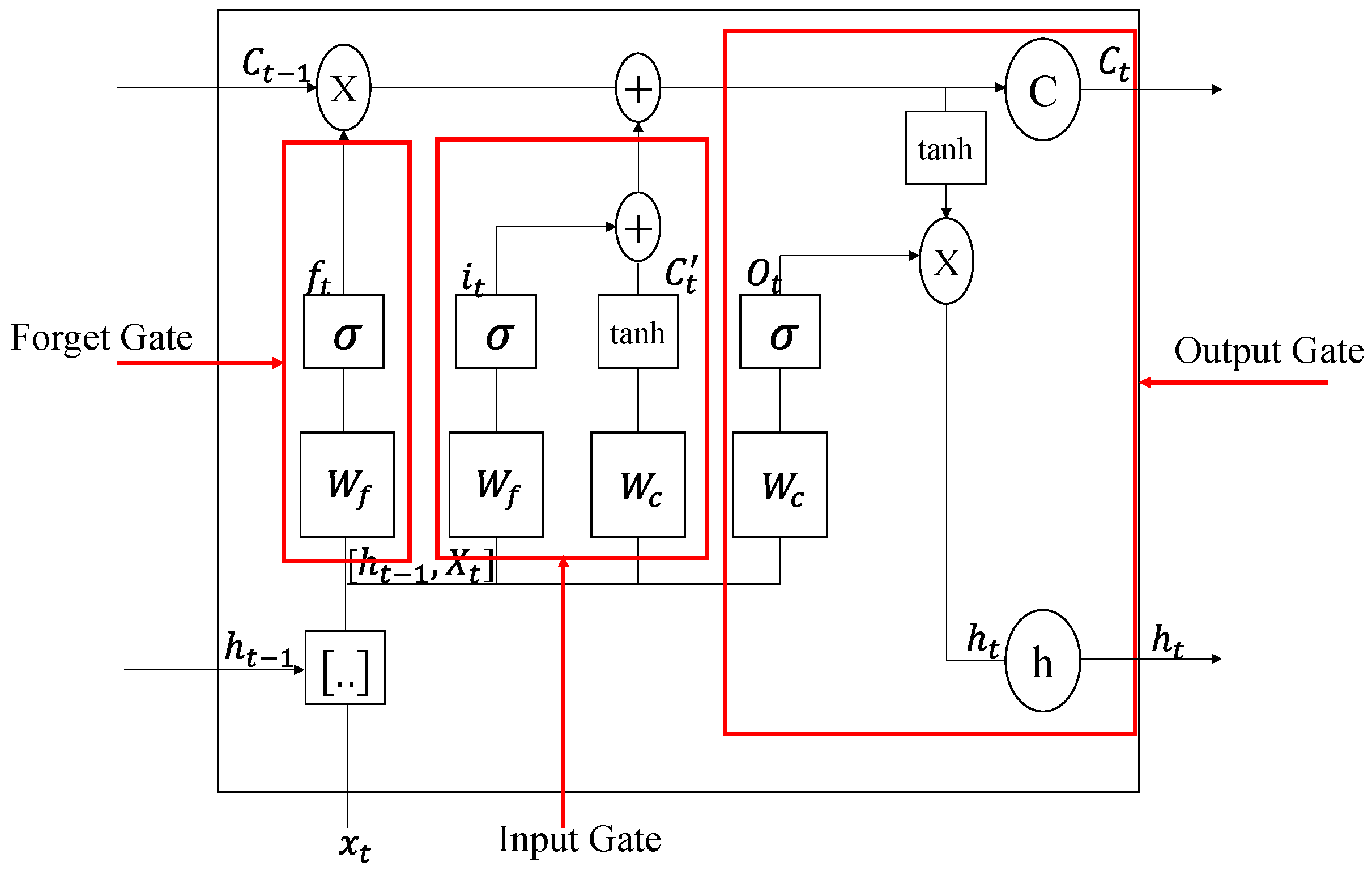
2. Long Short-Term Memory (LSTM) Neural Networks

Long short-term memory is an excellent variant of the recurrent neural network model. Proposed by Hochreiter and improved by several scholars, its excellent performance in processing time series and nonlinear system problems means it is widely used in natural language processing and data mining [25]. Its effective handling of the problem of RNN gradient explosion or disappearance makes it one of the most advanced deep-learning architectures for sequence learning tasks [26]. The internal structure of its unit is shown in Figure 1.

$f_t$, $i_t$, $C_t$, and $O_t$ in Figure 1 represent the forgetting gate, input gate, output gate, and output moment, respectively; w, tanh, and b are corresponding weight coefficients, the excitation function, and the deviation amount, respectively. The forgetting gate decides how many state units ($C_{t-1}$) from the last moment are kept to the moment ($C_t$), and its input ($x_t$) and output ($h_{t-1}$) from the previous moment are combined with the state unit ($C_{t-1}$) through the sigmoid function to determine the forgetting content; the input gate determines how much of the input ($x_t$) from the network at the current moment is kept in the state unit ($C_t$), and the input gate can avoid unimportant information from entering the memory, where the input ($x_t$) and output ($h_{t-1}$) of the current moment are combined with the tanh function to produce a new memory, that is, the intermediate vector ($C_t$). Combined with the output ($i_t$) of the sigmoid function, this controls the addition of new information; the output gate controls ($C_t$) how much of the state unit has output to the current output ($h_t$) value of the LSTM model. The operation mechanism is shown in Equations (1)–(6) [27].

Retention of forgotten gate control information:

$$f_t=\sigma \left(w_f\cdot \left[h_{t-1},x_t\right]+b_f\right)$$

(1)

Storage of updated information:

$$i_t=\sigma \left(w_t\cdot \left[h_{t-1},x_t\right]+b_i\right)$$

(2)

$$C^{\prime }=\tanh \left(w_c\cdot \left[h_{t-1},x_t\right]+b_c\right)$$

(3)

Aggregate input information and update information:

$$C_t=f_t\cdot C_{t-1}+i_t\cdot {C^{\prime }}_t$$

(4)

Determine the output information:

$$O_t=\delta \left(w_o\cdot \left[h_{t-1},x_t\right]+b_o\right)$$

(5)

Output information activation:

$$h_t=O_t\cdot \tanh \left(C_t\right)$$

(6)

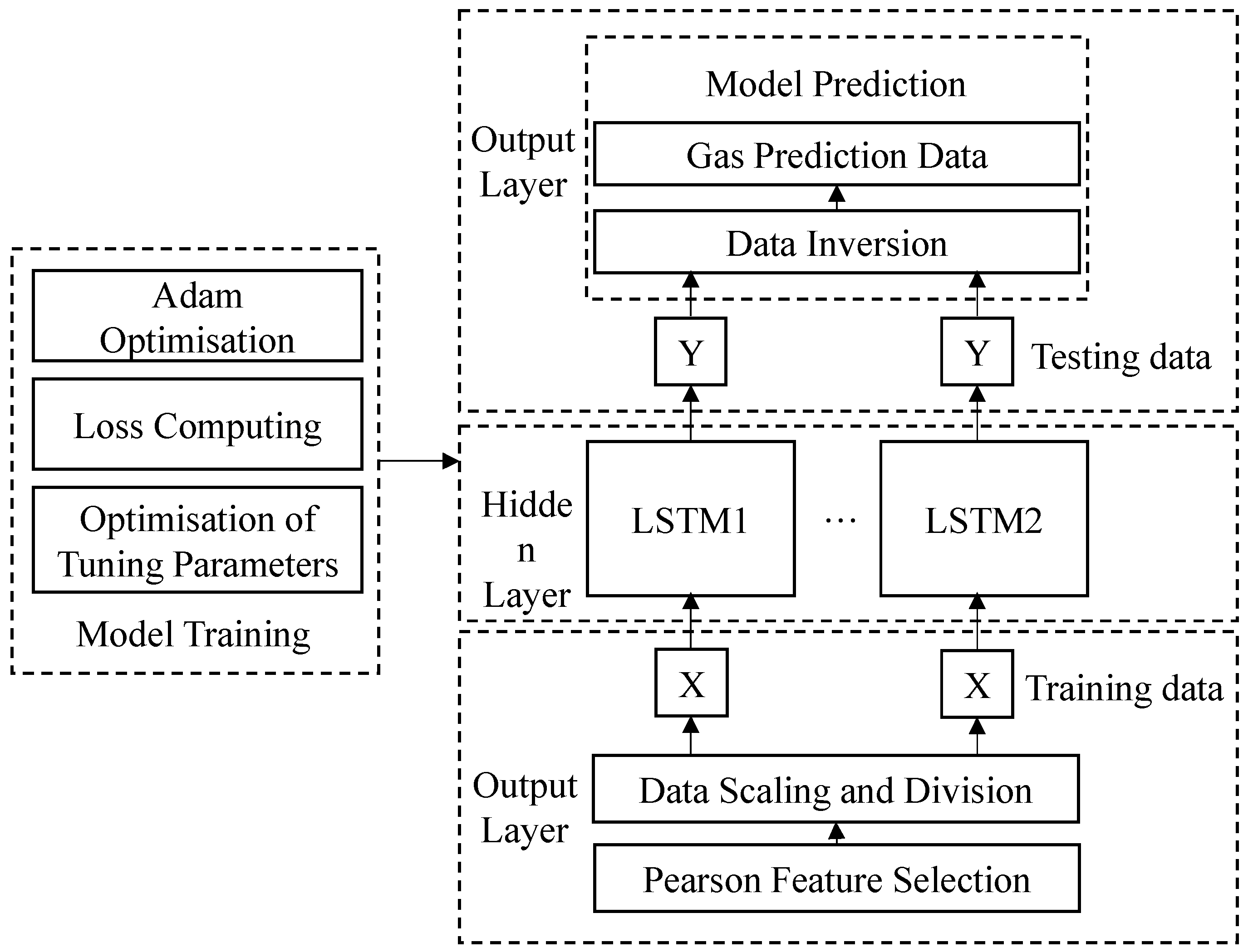
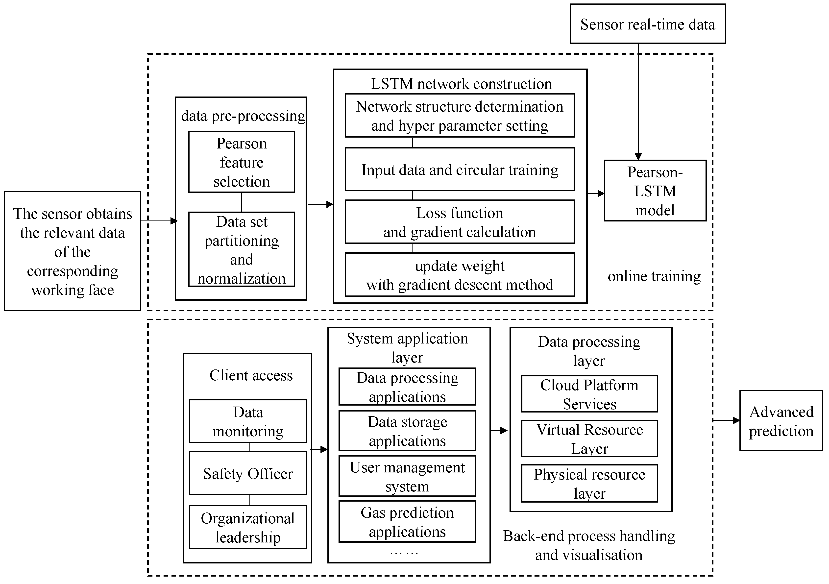
3. Construction of a Gas Concentration Prediction Model in a Working Face

Statistical methods are more representative of the correlations between data than machine learning feature selection methods, such as Relief, Lasso regression, and Random Forest. One of the most representative measures of data correlation is Pearson analysis, which is the fundamental reason we used Pearson coefficients in this study. The Pearson correlation coefficient measures the degree of correlation between the main indicator and the eigenvalue. The coefficient is between −1 and +1, and the larger the absolute value, the stronger the correlation. A negative value indicates the opposite change trend between the main indicator and the feature, and a positive value indicates the same change trend between the two.

Pearson correlation coefficient-based neural network models for long short-term memory (Pearson-LSTM) can be divided into three parts: the input layer, the hidden layer, and the output layer. The model runs as shown in Figure 2. First, the input layer performs Pearson feature selection, shrinkage treatment, and dataset-partitioning on the original data.

The deflation uses the MinMaxScaler normalization formula to run the principle as shown in Equations (7) and (8).

$$X_{std}=\frac{\left(X-X_{Min}\right)}{\left(X_{Max}-X_{Min}\right)}$$

(7)

$$X_{scaled}=X_{std}\cdot \left(Max-Min\right)+Min$$

(8)

In the formula, $X_{\mathit{Max}}$ indicates the series maximum, and $\mathit{Max}$ and $Min$ indicate the final size range.

The training set is trained based on the hidden layer, and the LSTM neural network weights are continuously updated by the Adam optimization algorithm to optimize the model based on the principle of minimizing the value of losses.

Finally, the optimal structure and parameter combinations are obtained by continuously adjusting the number of network layers and the batch size and using the Relu activation function to enhance the computational capacity. Dropout is added to prevent overfitting, and the output layer predicts the data based on the model trained in the hidden layer, thus reducing the data.

4. Example Analysis

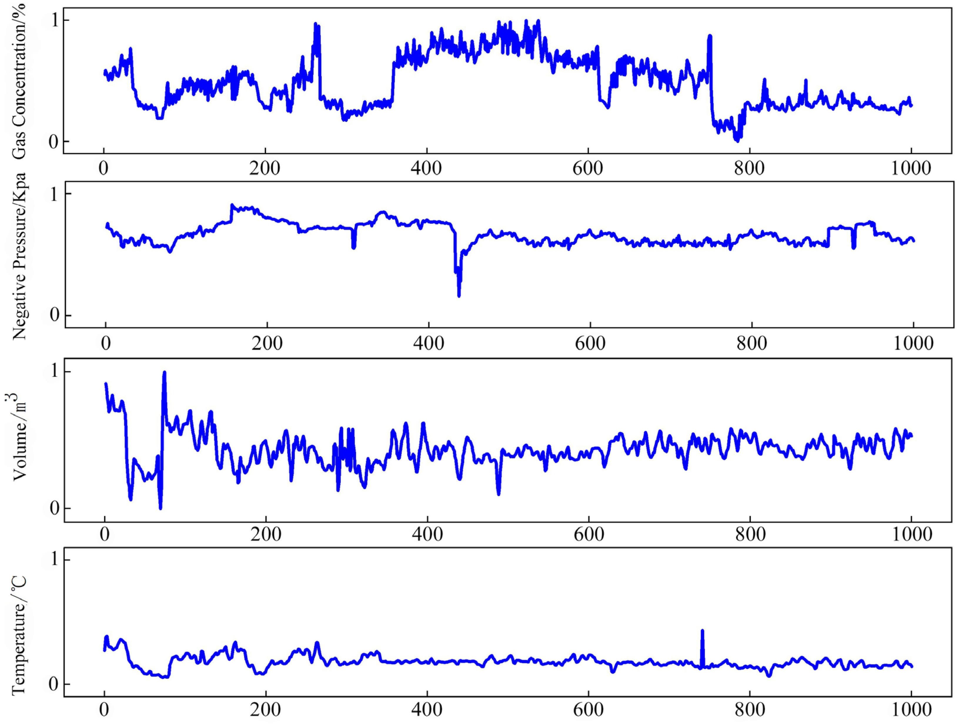
4.1. Correlation Analysis

To make better use of the Pearson-LSTM model, we applied it to the Yuhua Coal Mine of Shaanxi Coal Tongchuan Mining Co. Yuhua Coal Mine mainly mines the 4# coal seam, with a maximum coal seam gas content of 5.4 m³/t, a minimum of 3 m³/t, and an average of 4.2 m³/t. The maximum gas resolution is 2.7 m³/t, the minimum is 0.69 m³/t, and the average is 1.695 m³/t, which means that it is a high-gas mine. The coal seam thickness ranges from 3 to 12 m, with an average thickness of 7.5 m. The coal seam mining process is top coal mining, and the coal mine advances approximately 6 m per day, which is a strong disturbance to the overburden of the working face [28].

We used the daily production monitoring data of the 2407 working face at Yuhua Coal Mine, recorded from 20 March to 2 April 2021. The data include eight indexes, working face gas concentration, gas concentration in the upper corner, return air gas concentration, temperature, pure volume, negative pressure, carbon monoxide concentration, and carbon dioxide concentration [29], with a sampling interval of 15 min and 1000 datasets.

The gas concentration at the working face was taken as the explanatory variable, and all explanatory variables were divided using Pearson coefficients to find the high, moderate, low, and irrelevant variables in the explanatory variables. The results of the coefficients are shown in

Table 1. Pearson correlation coefficients.

Correlation Strength	Indicators	Pearson Coefficient
High correlation	Temperature	0.882
	Drainage negative pressure	0.841
	Pure volume	0.802
Moderate correlation	Gas concentration in upper corner	0.562
	Return air gas concentration	0.523
Low correlation	CO concentration	0.357
	CO2 concentration	0.198

.

According to the magnitude of the coefficients temperature, negative pressure and pure volume are highly correlated, indicating that these three explanatory variables are significantly linked to the explanatory variable work-surface gas concentration and inherently necessary. To avoid the LSTM model’s running time lengthening and accuracy degradation due to too many indicators, we eliminated the moderate and low correlated characteristic indicators, and took the highly correlated indicators as the final explanatory variables, with the explanatory variables themselves as the inputs to the model.

4.2. Data Preprocessing

The Pearson coefficient filtered data were divided into a validation set, a training set, and a test set in a ratio of 2:6:2, and then the data were cleaned up by supplementing the missing data with approximate averages and removing abnormal data. The data were normalized by using the MinMaxScaler method in Section 3 and scaled to [0, 1] for easier calculation and improved accuracy; the processed data are shown in Figure 3.

The computer configuration used for this experiment was as follows: an Intel Core CPU (i7-8550U) processor running at 1.80 GHz/2.00 GHz, 16 GB RAM, Windows 10 Home Edition (64-bit). The program was designed using the Python 3.7 development language, PyCharm Community Edition Integrated Development Environment. The LSTM model used in the development of the program was from the Keras deep-learning framework package with TensorFlow as the backend. The mean squared error (MSE) was used as an indicator of the precision of the model, as shown in Equation (9).

$$MSE=\frac{1}{n}{\displaystyle \sum _{i=1}^n{\left(f_i-y_i\right)}^2}$$

(9)

In the formula, f_i indicates the predicted value; y_i indicates the true value.

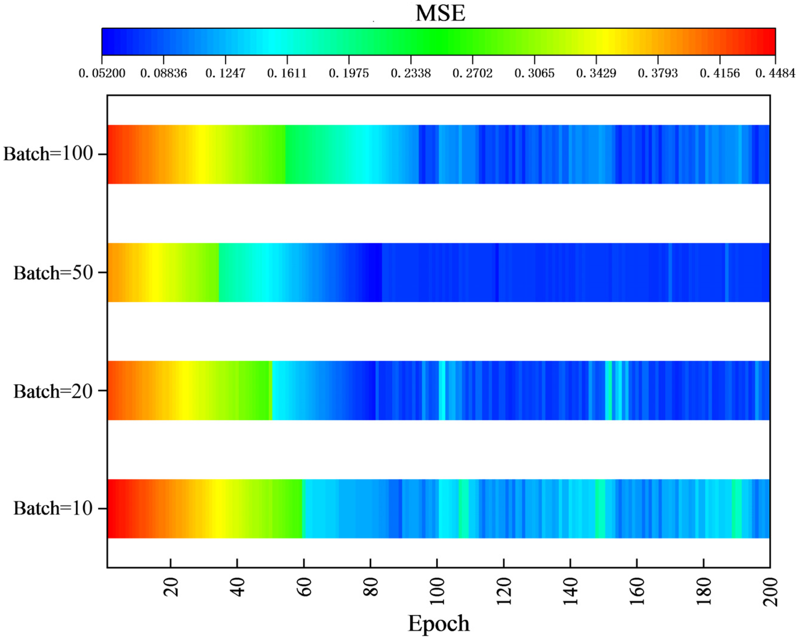
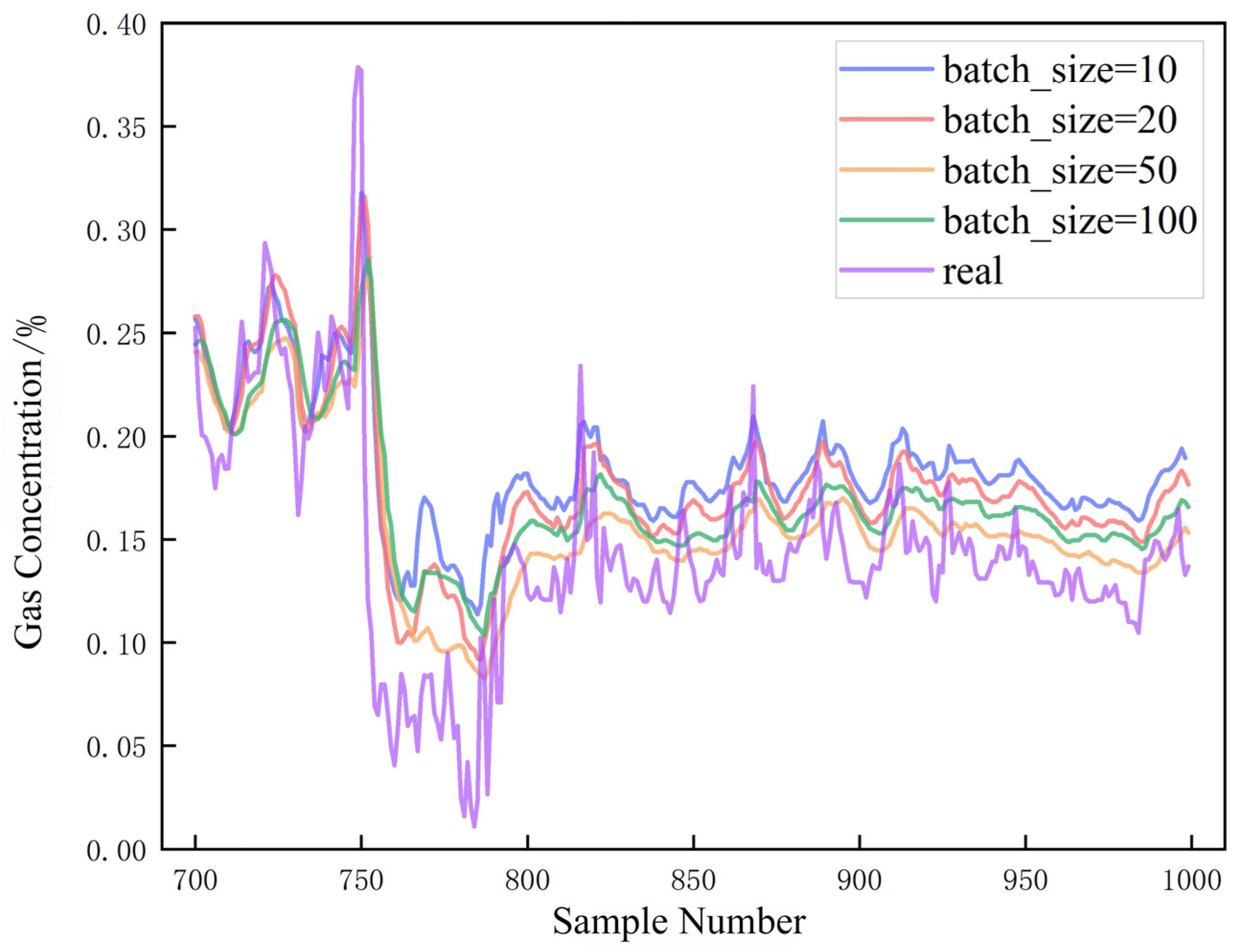
4.3. Batch Size Tuning

The batch size represents the length of sequences that the LSTM can utilize, and it is a response to the size of the data selected by the neural network and the degree of data association. The batch size determines the direction of gradient descent: too large, and it leads to a stable gradient direction change, and it is easy for it to fall into the local optimal solution; too small, and it leads to difficult convergence, thus affecting the model accuracy. Therefore, the selected batch size must meet the application requirements of the model.

Therefore, to research the influence of batch size on the model, we selected samples numbered from 700 to 1000 for this experiment and adopted a broad strategy of gradually increasing the batch size. The neuronal number was set to 128 to prevent overfitting, and the Epoch was set to 200 to make the model loss value decrease sufficiently and compare the effect of batch sizes of 10, 20, 50, and 100.

From Figure 4 and Figure 5, it can be seen that when the batch size is 50, the loss value is significantly lower than that of batch sizes 10, 20, and 100, and the loss value decreases the fastest during iterations without significant oscillations. Thus, prediction fit is the best. As can be seen from

Table 2. Batch size prediction results.

Neuronal Number = 128
Batch	Operation Time	MSE
10	7 min	0.1203
20	5 min	0.0912
50 100	4 min 2 min	0.0731 0.0913

, a batch size of 50 has the smallest mean square error, although the run time is not the shortest. The predictive ability of gas concentration prediction models can be improved with an increase in batch size. However, when the batch size increases to a certain size, the accuracy and imitative effect of the model decreases even if the run time is shortened. Considered comprehensively when the batch size is 50, the model has the greatest predictive power with a run time of about 4 min and an error of 0.008.

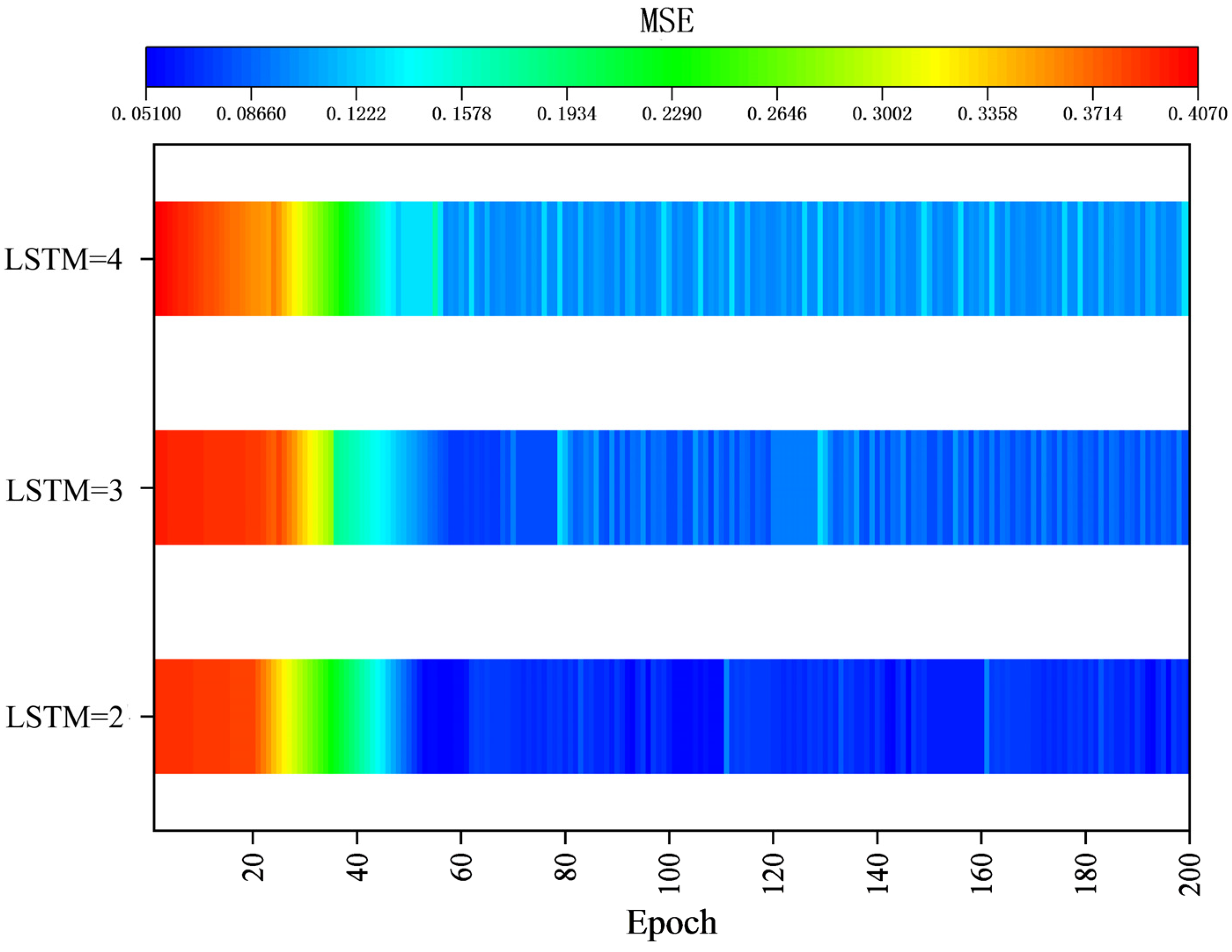
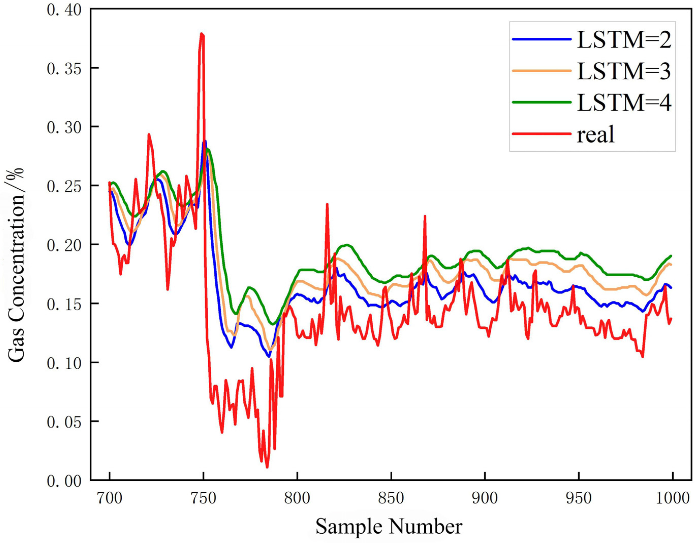
4.4. Network Layer Tuning

Theoretically, the more hidden layers, the better the fitting ability, but with an increase in layers, the structure will become more complex and harder to train, and there may be an overfitting situation, worsening the generalization ability. In this paper, we compared the effects of two-layer, three-layer, and four-layer LSTMs. The experimental results are shown in Figure 6 and Figure 7 and

Table 3. LSTM layer prediction results.

Batch Size = 50    Neuronal Number = 128
LSTM Layers	Operation Time	MSE
2	4min	0.0587
3 4	5min 8min	0.0801 0.1292

.

Figure 6 shows the results of the comparative analysis of the loss values for different layers. From Figure 6, it can be seen that the two-layer LSTM continues to maintain a low loss value range during the iterative process, with no significant fluctuations compared to the three- and four-layer LSTMs. Figure 7 shows the fitting results with different numbers of layers. The prediction results of the three- and four-layer models are slightly higher than the actual values, but the prediction results of two-layer LSTM are closer to the real data values. Table 3 shows that the two-layer LSTM has the shortest runtime and the smallest error. The model’s learning ability increases with the increase in the number of LSTM layers, but the precision of its predictions decreases, and the running time increases. The prediction effect of the LSTM model with two hidden layers is optimal when considered together.

Both the batch size and the size of the network layers have a significant impact on the model’s training time, testing time, and learning ability. An appropriate combination of parameters can significantly improve the model performance when multivariate fusion inputs are used. In this study, a batch size of 50 and 2 hidden layers are the best parameters for a working face gas concentration prediction model, and the model can better forecast the gas concentration change trends after training.

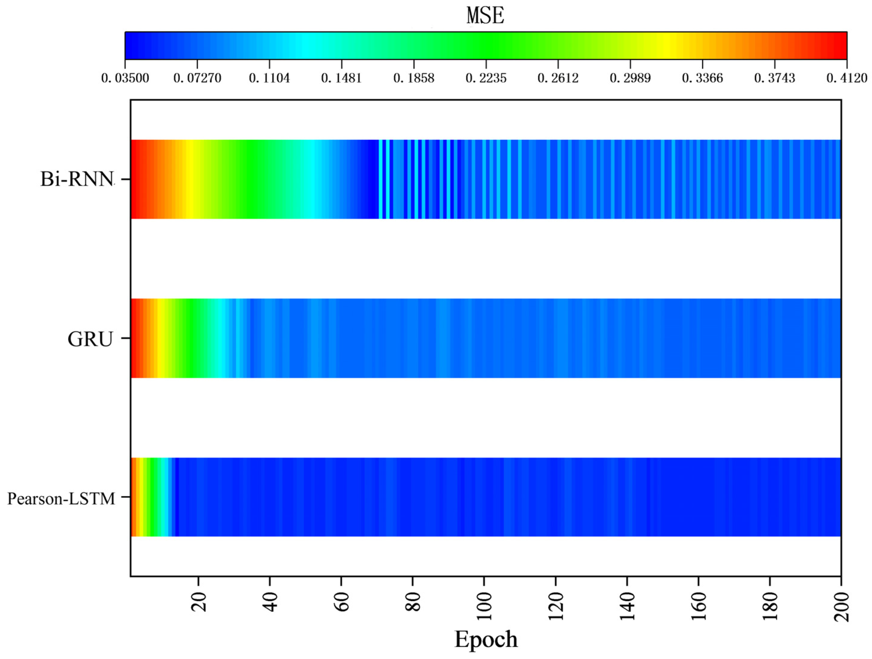
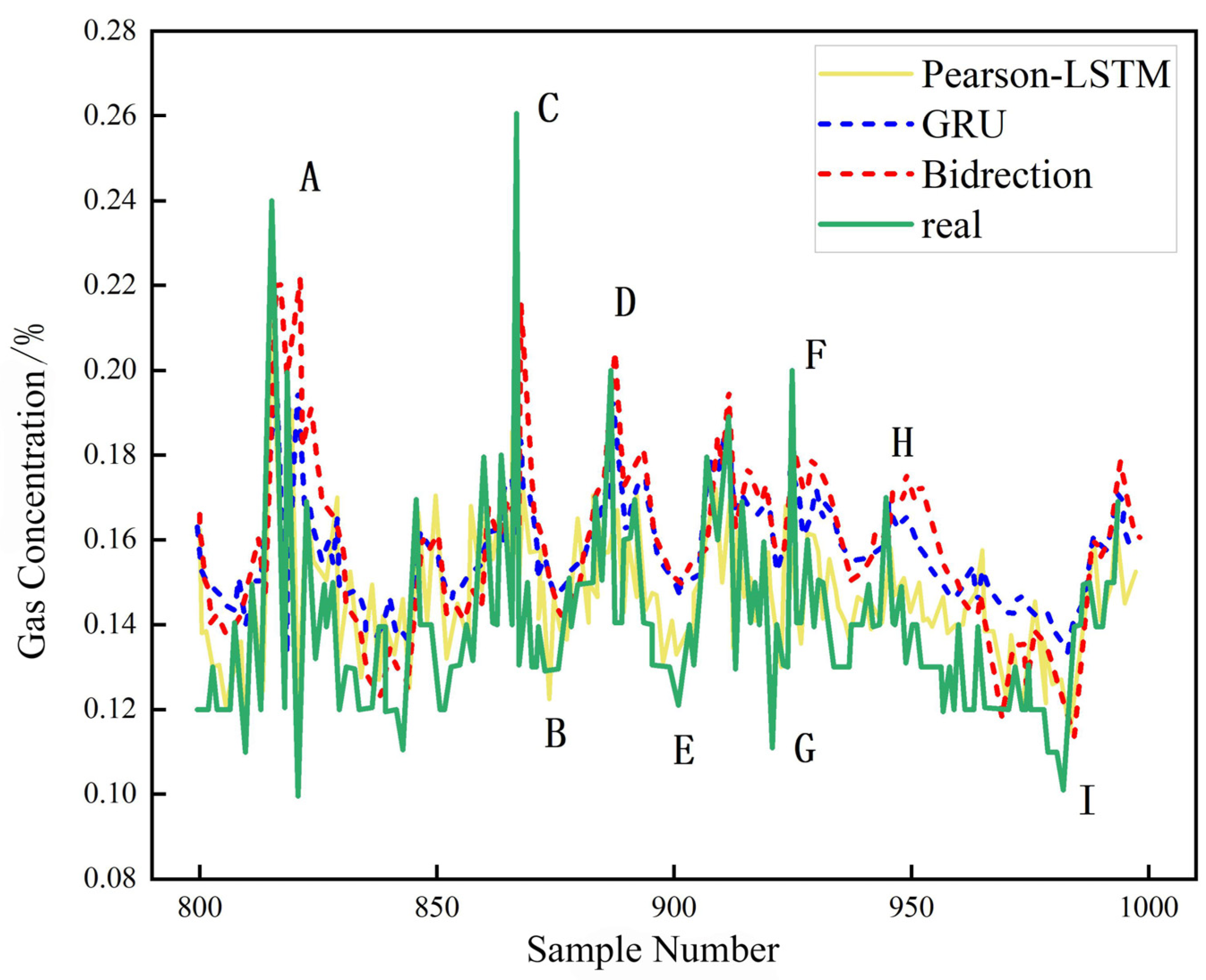
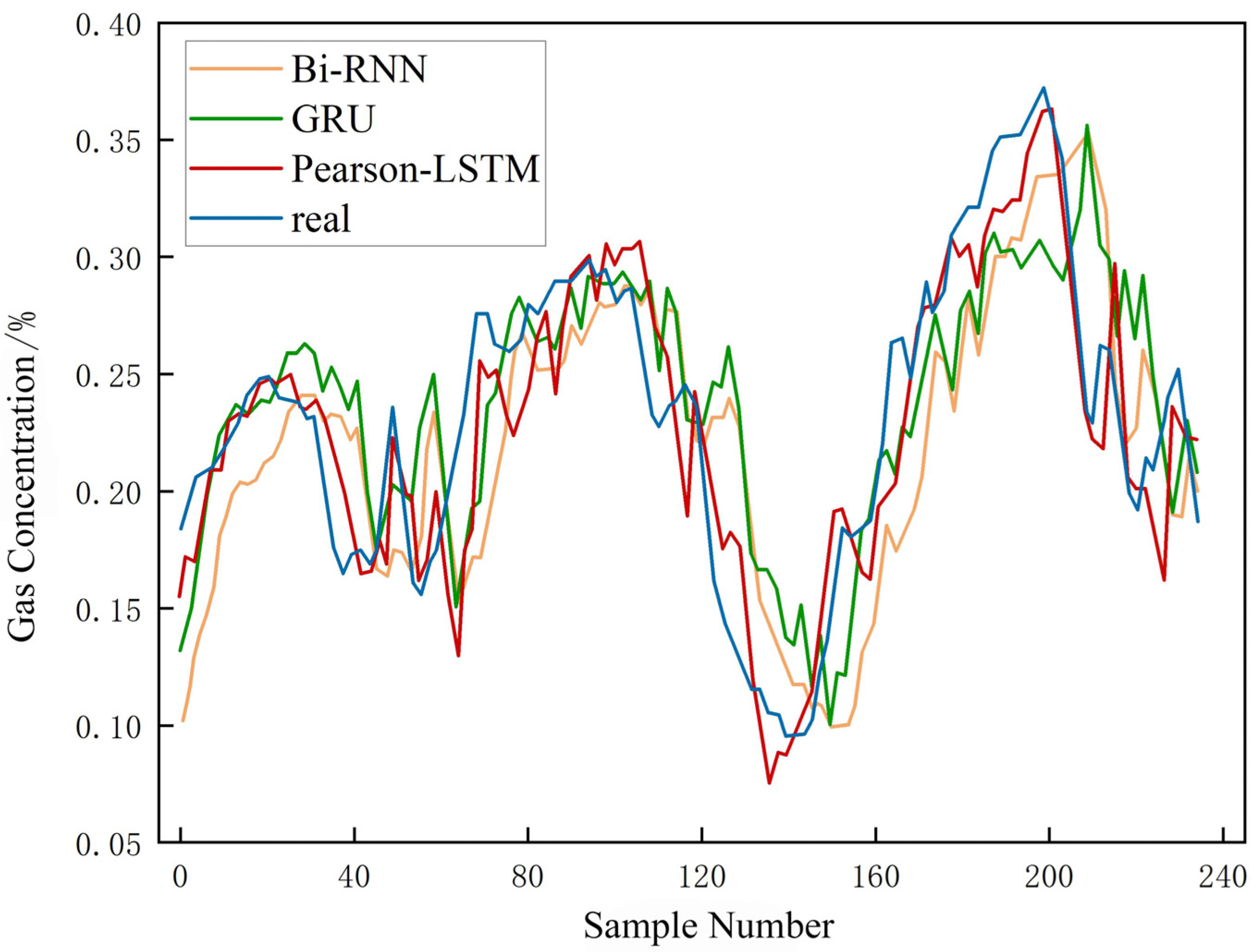
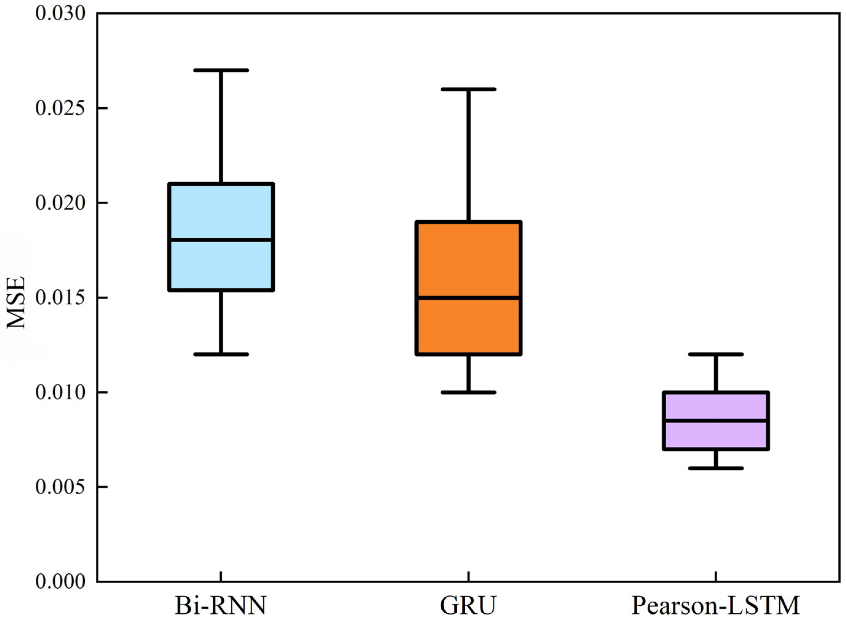
4.5. Model Comparison Analysis

To verify the superiority of the Pearson-LSTM model, in this experiment, the hidden layer structure of the Pearson-LSTM model’s main training layer was replaced by the Bi-RNN [30,31] and GRU [32,33] structures. The test set was selected and performed with the same parameters. The results are shown in Figure 8 and Figure 9 and

Table 4. Comparison of operation results.

Parameter Setting	Batch Size = 50; Layers = 2; Neuronal Number = 128
model	Pearson-LSTM	GRU	Bi-RNN
operation time	5569 s	4540 s	18,640 s
MSE	0.0521	0.0689	0.0801

.

Table 4 shows that Bi-RNN has the longest run time among the three models, and as shown in Figure 8, Pearson-LSTM is the most stable during the iterations, with the fastest decrease in error compared with GRU and Bi-RNN. In Figure 9, GRU and Bi-RNN can fit only the peaks of A, C, D, F, and H efficiently, but the fitting effect at the valley values of B, E, G, and I are much smaller than those of the Pearson-LSTM model. Compared with GRU and Bi-RNN, the Pearson-LSTM model can effectively accommodate the general gas concentration trend, as well as the peaks and valleys, and it has the lowest error rate in terms of predicting the trend change process with minimum error.

This paper compared the overall fitting results of GRU and Bi-RNN to verify the superiority of the Pearson-LSTM model in a deeper way, as shown in Figure 10, Figure 11 and Figure 12 and

Table 5. Comparison of prediction results.

Model	Maximum Error	Minimum Error	Mean Error
Pearson-LSTM	0.046283	0.00589	0.015479
GRU Bi-RNN	0.063648 0.073761	0.00916 0.0372	0.04246 0.042919

.

In the gas concentration time series, the overall trend was predicted by all three models; however, compared with Bi-RNN and GRU, the Pearson-LSTM model has a better overall fitting effect. A detailed comparison of the forecast data errors is shown in Table 5. The Bi-RNN and GRU prediction models are almost identical, with an average mean square error of approximately 0.02. The Pearson-LSTM prediction model has good saturation and greater precision, and the average mean square error could be lowered to 0.015, with an error range of 0.005 to 0.04.

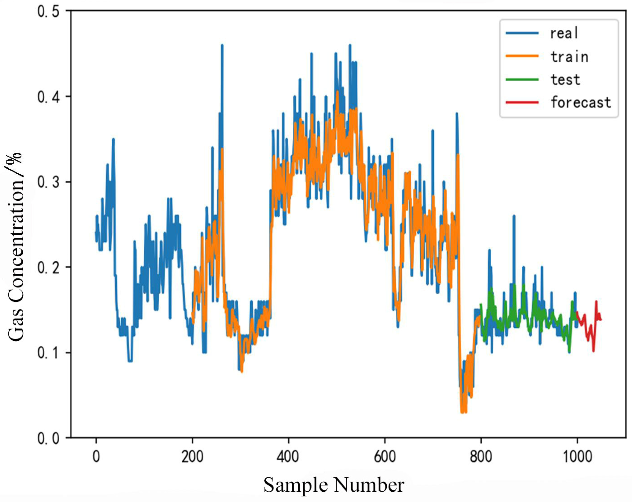
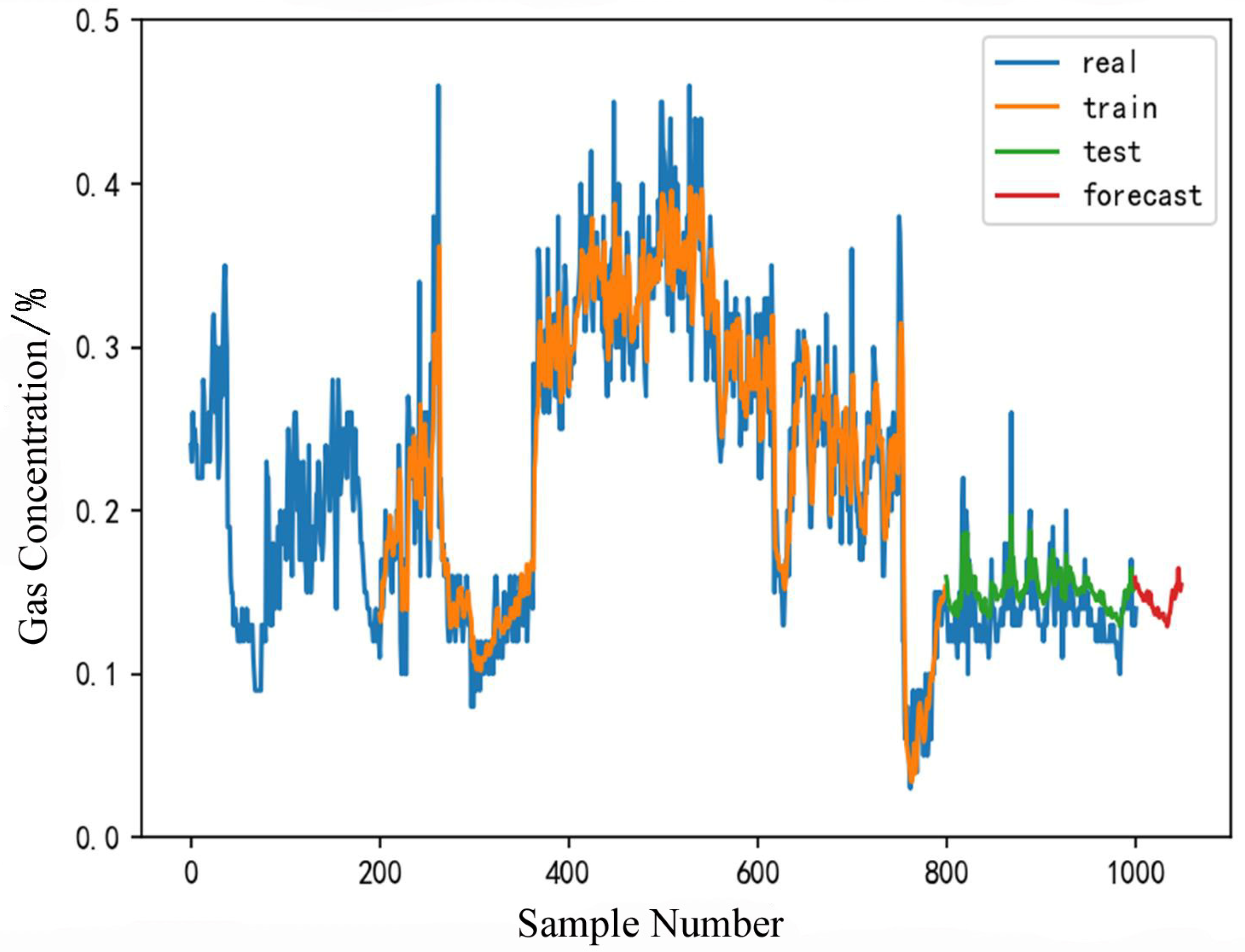
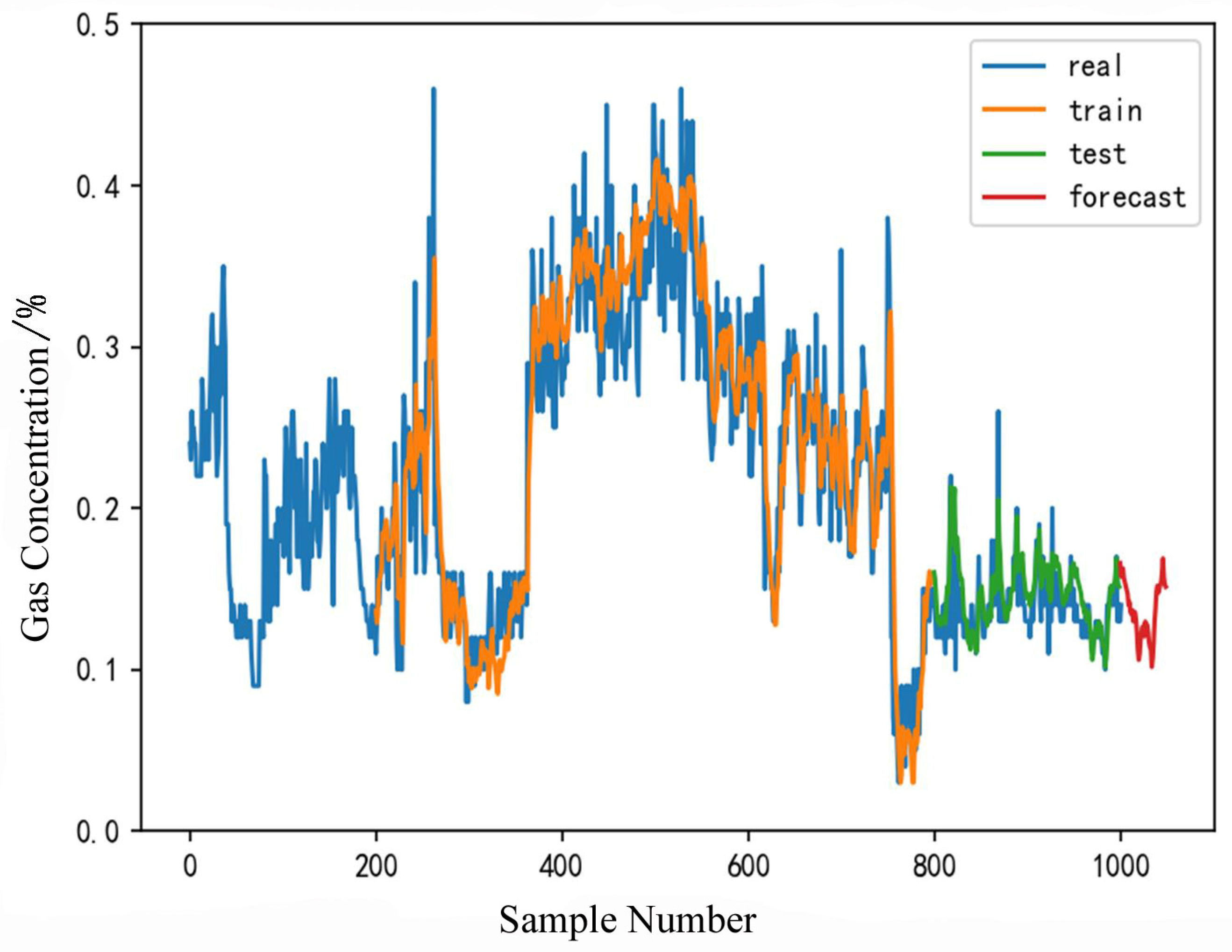
4.6. Application Effect Investigation

To verify the suitability and credibility of the working face gas concentration prediction model presented in this paper, we used the Keras deep-learning framework with TensorFlow as the main backend to implement the model’s online training as shown in Figure 13. First, the data were acquired using a sensor for Pearson feature selection and normalization. Second, the LSTM grid model with two hidden layers and a batch size of 50 was constructed based on the results of the model tuning in Section 3. The preprocessed data were fed into the network for training, during which the gradient and loss values were calculated, and their weights were updated continuously. Finally, the real-time sensor data were fed into the prediction model to obtain the predicted gas concentration value at the overburdened working face.

The 2407 and 2409 working faces are neighboring working faces, and their geology and mining conditions are basically the same. Using a sensor, the 2409 working face of the Yuhua Coal Mine was analyzed by the three models of Bi-RNN, GRU, and Pearson-LSTM models for advanced corresponding time outputs starting at 13: 10: 00 on 19 August 2021 at an interval of 15 min. By 01: 30: 00 on 22 August 2021, a total of 240 sets of results were selected. The predictions from the three models are shown in Figure 14. The models automatically calculated the errors after inputting the data, and the error calculation process is shown in Equation (10). The error statistics were plotted in a box plot, as shown in Figure 15, where the horizontal line in the middle of the box plot represents the mean value. The Pearson-LSTM model’s result is closer to the true value, with an average error of 0.008, which is 55.6% and 52.2% lower than Bi-RNN and GRU, respectively.

5. Conclusions

(1)

During the training process, the value of the target function, the fit, and the running time were influenced by the choice of batch size and the number of layers in the Pearson-LSTM model. An appropriate batch size and number of network layers can efficiently improve the model. An experimental Pearson-LSTM gas prediction model with a batch size of 50 and 2 hidden layers is the best combination to predict gas concentration with maximum accuracy.

(2)

The Pearson-LSTM model has a better predictive effect compared with traditional recurrent neural networks, such as Bi-RNN and GRU. Taking the prediction results of the 2407 working face of the Yuhua Coal Mine as an example, the average error of the model can be lowered to 0.015. The margin of error is 0.005~0.04, with high robustness.

(3)

The Pearson-LSTM gas concentration prediction model was employed to forecast gas concentrations at the 2409 working face of the Yuhua Coal Mine 15 min in advance, with an average error of 0.008. It demonstrated the reliability of the model and guaranteed the safety of daily coal mine operations. Thus, the reliability of the model has been fully demonstrated, proving that it can be applied to the coal mining process and can effectively predict gas concentrations. It can be promoted and applied to other coal mines to guarantee the safety of daily coal operations.

References

1. Cheng, J.; Bai, J.; Qian, J.; Li, S. Short-Term Forecasting Method of Coalmine Gas Concentration Based on Chaotic Time Series. J. China Univ. Min. Technol. 2008, 2, 231–235. [Google Scholar]
2. An, M.; Du, Z.; Zhang, L. Statistical analysis of coal mine gas accidents in China from 2007 to 2010. Saf. Coal Mines 2011, 5, 177–179. [Google Scholar]
3. Wang, H.; Wu, B.; Lei, B. Numerical simulation study on influence factors of gas accumulation at fully mechanized caving Face. Saf. Coal Mines 2018, 3, 151–154+159. [Google Scholar]
4. Fu, H.; Dai, W. Gas concentration dynamic prediction method of mixtures kernels LSSVM based on ACPSO and PSR. Chin. J. Sens. Actuators 2016, 6, 903–908. [Google Scholar]
5. Fu, H.; Feng, S.; Liu, J.; Tang, B. The modeling and simulation of gas concentration prediction based on De-Eda-Svm. Chin. J. Sens. Actuators 2016, 2, 285–289. [Google Scholar]
6. Wei, L.; Bai, T.; Fu, H.; Yi, Y. New gas concentration dynamic prediction model based on the EMD-LSSVM. J. Saf. Environ. 2016, 2, 119–123. [Google Scholar]
7. Fu, H.; Zi, H.; Meng, X.; Sun, L. A new method of mine gas dynamic prediction based on EKF-WLS-SVR and chaotic time series analysis. Chin. J. Sens. Actuators 2015, 1, 126–131. [Google Scholar]
8. Wu, Y.; Qiu, C.; Lv, X. Prediction of gas concentration based on fuzzy information granulation and markov correction. Coal Technol. 2018, 5, 173–175. [Google Scholar]
9. Yang, L.; Liu, H.; Mao, S.; Shi, C. Dynamic prediction of gas concentration based on multivariate distribution lag model. J. China Univ. Min. Technol. 2016, 3, 455–461. [Google Scholar]
10. Wu, Z.; Wu, X.; Qian, J. Trend prediction of gas concentration based on interpolation trapezoidal fuzzy information granulation. J. Mine Autom. 2014, 12, 31–36. [Google Scholar]
11. Wang, P.; Wu, Y.; Wang, S.; Song, C.; Wu, X. Study on Lagrange-ARIMA real-time prediction model of mine gas concentration. Coal Sci. Technol. 2019, 4, 141–146. [Google Scholar]
12. Lai, X.; Xia, Y.; Zheng, W.; Cui, J.; Wu, Y.; Shi, Y. Improved grey prediction of gas concentration sequence based on integrated learning. J. Saf. Sci. Technol. 2021, 7, 16–21. [Google Scholar]
13. Liang, Y.; Li, X.; Li, Q.; Mao, S.; Zheng, M.; Li, J. Research on intelligent prediction of gas concentration in working face based on CSLSTM. Min. Saf. Environ. Prot. 2022, 4, 80–86. [Google Scholar]
14. Wang, D.; Zhu, G.; Wang, Y.; Wang, S. Prediction Model of Gas Concentration in Fully Mechanized Mining Face Based on GA-LSTM. Coal Technol. 2023, 1, 219–221. [Google Scholar]
15. Qi, Y. Research on Coal Mine Gas Concentration Prediction Method Based on Information Fusion and GA-BP. Coal Technol. 2022, 6, 159–161. [Google Scholar]
16. Fan, J.; Huang, Y.; Yan, Z.; Li, C.; Wang, C.; He, Y. Research on gas concentration prediction driven by ARIMA-SVM combined model. J. Mine Autom. 2022, 9, 134–139. [Google Scholar]
17. Xu, N.; Wang, X.; Meng, X.; Chang, C. Gas Concentration Prediction Based on IWOA-LSTM-CEEMDAN Residual Correction Model. Sensors 2022, 22, 4412. [Google Scholar] [CrossRef]
18. Wang, D.; Zhao, L.; Hao, T.; Du, Y.; Shen, J.; Tang, Y.; Gong, J.; Li, F.; Yan, X.; Yan, Z.; et al. Multiple Sequence Long and Short Memory Network Model for Corner Gas Concentration Prediction on Coal Mine Workings. ACS Omega 2022, 7, 37980–37987. [Google Scholar] [CrossRef]
19. Jia, P.; Liu, H.; Wang, S.; Wang, P. Research on a Mine Gas Concentration Forecasting Model Based on a GRU Network. IEEE Access 2020, 8, 38023–38031. [Google Scholar] [CrossRef]
20. Zhang, Z.; Ye, Y.; Dong, L. A Graph Neural Network gas concentration prediction model based on Spatio-Temporal data. J. Phys. Conf. Ser. 2021, 8, 2137. [Google Scholar] [CrossRef]
21. Tian, H.; Zhang, Z.; Yu, D. Research on multi-load short-term forecasting of regional integrated energy system based on improved LSTM. Proc. CSU-EPSA 2021, 9, 130–137. [Google Scholar]
22. Dai, J.; Song, H.; Sheng, G.; Jiang, X. Prediction method for power transformer running state based on LSTM network. High Volt. Eng. 2018, 4, 1099–1106. [Google Scholar]
23. Zheng, Y.; Wang, H. Study on short-term road traffic flow prediction based on deep learning. Software 2020, 5, 72–74. [Google Scholar]
24. Liu, Y.; Yang, C. LSTM gas concentration prediction model based on multiple factors. J. Saf. Sci. Technol. 2022, 1, 108–113. [Google Scholar]
25. Park, C.; Choi, K.; Lee, C.; Lim, S. Korean coreference resolution with guided mention pair model using deep learning. Etri J. 2016, 6, 1207–1217. [Google Scholar] [CrossRef] [Green Version]
26. Li, F.; Chen, Y.; Xiang, W.; Wang, J. State degradation trend prediction based on quantum weighted long short-term memory neural network. Chin. J. Sci. Instrum. 2018, 7, 217–225. [Google Scholar]
27. Jian, Z.; Troyanskaya, O.G. Predicting effects of noncoding variants with deep learning-based sequence model. Nat. Methods 2015, 10, 931–934. [Google Scholar]
28. Sun, B.; Li, X.; Fan, F. Precise detection technology for gas enrichment characteristics of overburden rock under pressure of strong mining in thick coal seam. Saf. Coal Mines 2022, 6, 75–82+88. [Google Scholar]
29. Klyuev, R.V.; Bosikov, I.I.; Gavrina, O.A. Cluster analysis of electric energy consumption in metallurgy enterprises. In Advances in Raw Material Industries for Sustainable Development Goals; Taylor & Francis Group: London, UK, 2021; pp. 377–385. ISBN 978-0-367-75881-3. [Google Scholar]
30. Hao, Z.; Hao, H.; Ruichu, C.; Ruichu, W. Fine-grained opinion analysis based on mul-ti-feature fusion and bidirectional RNN. Comput. Eng. 2018, 7, 199–204+211. [Google Scholar]
31. Liang, L.; Li, J.; Zhang, S. Hyperspectral images classification method based on 3D octave convolution and Bi-RNN attention network. Acta Photonica Sinca 2021, 9, 284–296. [Google Scholar]
32. Li, X.; Duan, H.; Xu, M. A gated recurrent unit neural network for chinese word segmentation. J. Xiamen Univ. 2017, 2, 237–243. [Google Scholar]
33. Wang, J.; Wen, X.; He, Y.; Lan, J.; Zhang, C. Logging curve prediction based on a CNN-GRU neural network. Geophys. Prospect. Pet. 2022, 2, 276–285. [Google Scholar]
Figure 1. LSTM structural unit diagram.
Energies 16 02318 g001
Figure 2. Pearson-LSTM gas prediction model framework.
Energies 16 02318 g002
Figure 3. Processed data.
Energies 16 02318 g003
Figure 4. Comparison of batch size losses.
Energies 16 02318 g004
Figure 5. Comparison of batch size fitting effects.
Energies 16 02318 g005
Figure 6. Comparison of LSTM layer losses.
Energies 16 02318 g006
Figure 7. Comparison of LSTM layer number fitting effects.
Energies 16 02318 g007
Figure 8. Loss comparison for the three models.
Energies 16 02318 g008
Figure 9. Test results comparison for the three models.
Energies 16 02318 g009
Figure 10. Pearson-LSTM prediction model fitting effect diagram.
Energies 16 02318 g010
Figure 11. GRU prediction model fitting effect diagram.
Energies 16 02318 g011
Figure 12. Bi-RNN prediction model fitting effect diagram.
Energies 16 02318 g012
Figure 13. Advanced prediction scheme of gas concentration in the working face.
Energies 16 02318 g013
Figure 14. Comparison of the 15-min prediction results of the three models.
Energies 16 02318 g014
Figure 15. Box diagram of the prediction errors of the three models.
Energies 16 02318 g015