A Review on Process Modeling and Simulation of Cryogenic Carbon Capture for Post-Combustion Treatment

Abstract

The cryogenic carbon capture (CCC) process is a promising post-combustion CO₂ removal method. This method is very novel compared with conventional and well-developed methods. However, cryogenic carbon capture is not yet commercially available despite its techno-economic benefits. Thus, a model-based design approach for this process can provide valuable information. This paper will first introduce the cryogenic carbon capture process. Then, a comprehensive literature overview that focuses on different methods for modeling the process at the component level will be given. The modelling methods which are deemed most effective are presented more in depth for each of the key system components. These methods are compared with each other in terms of complexity and accuracy and the simplest methods with an acceptable level of precision for modelling a specific component in the CCC process are recommended. Furthermore, potential research areas in modeling and simulation of the CCC process are also highlighted.

1. Introduction

Due to population expansion, the world’s growing economy, and increasing urbanization, the global energy demand has been increasing exponentially [1]. Although renewables are expanding at high rates, they still cannot satisfy the global energy demand, and because of that, 80% of the current energy demand is still supplied by fossil fuels [2]. The large-scale use of fossil fuels has resulted in air pollution and has deteriorated human health. Based on a recent analysis, global CO₂ emissions increased from 33.3 Gigatons/year in 2020 to 34.9 Gigatons/year in 2021 [3]. This prompt increase in global CO₂ emissions has brought about numerous intense problems including climate change, global warming, rising sea level, etc. Using renewable energy systems, increasing the efficiency of energy conversion systems, and utilizing CO₂ capture technologies are the most practical solutions to regulate CO₂ emissions [4]. The latter method is very advantageous, especially in cases such as cement production where the emissions are not avoidable. This method directly targets the emissions at the source and may also remove other pollutants such as NO_x. Moreover, the integration of CO₂ capture technologies within large industrial plants is convenient and, in some cases, no fundamental change in the plant structure is required. For instance, the cryogenic carbon capture process is a bolt-on retrofit technology since the process just uses electricity, while amine-based processes just need heat and process integration. This technology can also provide an opportunity to supply and store CO₂ with high purities which can be used in fuel production or oil recovery processes. Pre-combustion, oxyfuel combustion, and post-combustion are three available CO₂ capture methods.

In the case of using the pre-combustion capture method, CO₂ is removed from a gas mixture prior to combustion [5]. In other words, hydrocarbon fuel is converted into carbon monoxide and syngas. Then, the generated carbon monoxide reacts with steam to produce hydrogen and CO₂. Finally, the produced CO₂ is separated from hydrogen that can be combusted without generating any pollutant. This technology is beneficial since it is verified for industrial-scale oil refineries, and it can recover 90–95% of CO₂. However, it requires high investment costs. Moreover, high NO_x emissions need expensive scrubbers.

In the oxyfuel process, as the name indicates, pure oxygen is used rather than air in the combustion chamber, which results in generating flue gases that consist of almost pure CO₂ and vapor. As a result, the separation, and purification of CO₂ in this method is very simple [6]. Therefore, CO₂ is captured and stored just by the condensation of vapor content in the flue gas and low-temperature purification. When this method is applied, a plant should be equipped with an air separation unit (for oxygen production), a flue gas processing unit as well as a CO₂ processing unit. This method can be considered rewarding since it results in very low emissions of NO_x, and it has high flexibility for using different types of fuels. Furthermore, achieving 100% combustion of biomass, better behavior of the combustion process, and using a smaller furnace are other attractive features of oxyfuel. However, replacing O₂ with air may bring about some challenges. In other words, the energy requirement for oxygen production is high, and keeping the flame stable is challenging [6,7]. Therefore, the net power production from the plant will be lower and flue gas should be recycled in large quantities to keep the temperature at reasonable levels.

Post-combustion CO₂ capture methods include chemical absorption, physisorption, membrane-based capture processes, and cryogenic carbon capture (CCC) processes. In the CCC process, gaseous CO₂ can be separated from other components in the flue gas due to their different condensation and desublimation temperatures. This method is gaining more popularity by using less energy [8,9,10,11,12,13,14,15], capturing CO₂ with higher rates and purities, and having faster responses to fluctuations in electricity demand [8,16,17]. Moreover, investigations have indicated that CO₂ capture costs can be decreased by 20–40% when the CCC process is used, and it distinctly indicates the economic advantages of the CCC process over other methods [18]. Furthermore, this technology can be easily added to the current industrial emission facilities without any concern regarding chemical solvents or physical sorbents [19]. This method can use natural gas as a refrigerant and because of that, it can store energy in the form of liquid natural gas (LNG). For capturing CO₂ using this method, only 12–18% of the power generated in the plant is consumed if the energy storage operates with efficiencies higher than 90% [8]. The energy supplied to the process is mostly used to drive compressors in refrigeration cycles mainly to liquefy natural gas and provide the required LNG for the process. The Cascade liquefaction cycle, mixed refrigerant cycle, and gas expander cycle are the available scenarios to liquefy natural gas and they are discussed in reference [20]. Despite all benefits and advantages of the CCC process, this technology is still in its early stages of development and deals with several challenges such as ice plugging when the flue gas is not water-free [15]. Moreover, this technology can be considered uneconomical when the CO₂ mole fraction in the gas mixture is very low. In this case, a large amount of gas other than CO₂ should be cooled to condense a very low amount of CO₂.

It should be noted that capture conditions have a great impact on the total costs and the required energy used for the separation and compression of CO₂ when the CCC process is used [21]. These conditions are the CO₂ concentration in flue gases, pressure, temperature, the chemical composition of flue gases, and the required purity of captured CO₂. However, among all aforementioned factors, the concentration of CO₂ in the flue gas affects the total costs and required energy more effectively.

Techno-economic evaluations have indicated that for large-scale applications, the CCC process costs are comparable with mature conventional monoethanolamine (MEA) absorption technology, while in smaller scales, the costs are significantly lower in the case of using the CCC process rather than MEA [22]. This process can generate extra LNG and store it when renewable electricity is available, or the plant power demand is low. The cooling energy stored in the form of LNG is then recovered during the peak hours when electricity is expensive. As shown in reference [16], using a tank with an LNG storage capacity of 8000 tons in the CCC process may result in alleviating the cycling costs regarding the load-following of power generation units by 85% when the maximum residential electricity demand is 2000 MW.

Exergy analysis, which is a powerful tool for evaluating the performance of thermal systems, can be used to improve the overall thermodynamic efficiency of the CCC process. The results of exergy analysis indicated that compressors and heat exchangers, especially water coolers, generate the total exergy loss in the process [23]. Under this situation, exergy loss of the process can be decreased by minimizing the temperature differences of heat exchangers and using multistage compressors with intercoolers which contribute to enhancing the performance of the process [24].

Although the CCC process is novel, different aspects of the process have been studied and investigated. The natural gas liquefaction process which is part of the CCC process has been extensively studied and evaluated. Nguyen et al. [25] compared mixed refrigerant cycles with expander-based systems. They concluded that the mixed refrigerant cycles are more efficient than the expander-based process under a wide range of operating conditions. In mixed refrigerant cycles, a mixture of hydrocarbons including methane, ethane, butane, ethylene, propane, and so forth with nitrogen might be used as a working fluid. In this case, a very low temperature in the range from −165 to −162 °C can be achieved when the refrigerant is expanded. Remeljej et al. [26] also indicated that using a single mixed refrigerant cycle is more advantageous than two open-loop expanders and two-stage expander nitrogen processes according to the results of exergy analysis. The dual mixed refrigerant process was also studied and investigated by Qyyum et al. [27]. They indicated that this cycle could produce LNG with high efficiency. However, the process possesses very high degrees of complexity. Moreover, this process is extremely sensitive to operating conditions and has very high capital costs. Kamath et al. [28] also provided an equation-based model which can be used to model multi-stream heat exchangers for cryogenic applications. This model utilizes pinch analysis and considers phase change by dividing the flows which may undergo the phase change into two sub-streams. Haider et al. [29] also represented a transient three-dimensional model which can be used as model plate-fin heat exchangers in cryogenic processes. This model is developed by computational fluid dynamics and correlations which are used to obtain pressure drop and heat transfer. An extended Peng Robinson equation of state was proposed by Martynov et al. [30] to calculate the solid–vapor equilibrium of CO₂. This model can be used to obtain phase equilibrium properties of CO₂ in solid/vapor phases including enthalpy, internal energy, thermal expansion, and heat capacity. Wibawa et al. [31] also evaluated the performance of the Peng Robinson Equation of State (PR EoS) and Vander Waals (vdW) mixing rules to calculate the solid–vapor equilibrium and liquid–vapor equilibrium of CO₂-CH₄. They also proposed a new binary interaction parameter for the solid–vapor equilibrium which is able to improve the accuracy of PR EoS. Ali et al. [32] also developed an artificial neural network technique for the solid–vapor equilibrium and solid–vapor–liquid equilibrium of binary CO₂-CH₄. This model is valid and can be used in a wide range of temperatures from −50 to −200 °C and different CO₂ concentrations from 1 to 54%. Reddy et al. [33] developed an empirical model based on real operational data which can be used to obtain the flow and power consumption of reciprocating compressors. This method can be used to model the compressors in natural gas liquefaction processes. Fang et al. [34] also reviewed the empirical models for centrifugal compressors. These models are very helpful for designing the energy analysis of the centrifugal compressors.

The available literature lacks a comprehensive review of mathematical approaches for modeling the CCC process and its main components. The main focus of the current study is to provide a numerical framework for modeling the main components of the CCC process. This review paper provides very helpful information about the performance of the CCC as well as primary information about the thermodynamics of the process, solid–vapor equilibrium, and liquid–vapor equilibrium. The fundamental information about the available models provided in this study can be effectively used to simulate, evaluate, and optimize the process. For each component in the process, the modeling approach along with the accuracy, advantages, and disadvantages are highlighted.

In this study, first the flue gas pre-processing is discussed. Then, the operation of the CCC process integrated with the energy storage is explained and different components and elements in the process are introduced. Afterwards, the available models and equation of states which can be used to model and investigate these elements including heat exchanger, bubbler, LNG storage tank, and compressor are discussed thoroughly. In particular, the differential method is discussed, which can be used to model the heat exchangers in the CCC process while the particle velocity model and pseudo-homogeneous one-dimensional plug flow model are given to model the desublimation heat exchanger. Different equation of states and models such as PR EoS, the Rachford–Rice equation, and SRK EoS are discussed which can be used to calculate the solid–vapor equilibrium and liquid–vapor equilibrium of CO₂ mixtures in the bubbler. The minimum energy model is also presented here which can be applied to calculate the minimum energy required to separate CO₂ from the flue gas in the bubbler. Furthermore, the RGibbS reactor block which is available in ASPEN Plus process simulator software is also introduced and its accuracy to calculate solid–vapor equilibrium is evaluated. Moreover, the volume of fluid and BWRS methods which can be used to model the LNG tank as an energy storage in the CCC process and calculate the boil-off-gas are also discussed. The compression process model of scroll compressors and the linear compressor model are also given to model and study the scroll compressors and linear compressors, respectively. This section is followed by the accuracy analysis section where a comprehensive comparison of the accuracy of different models in the literature is provided. Finally, this study is concluded, and the research gap is presented.

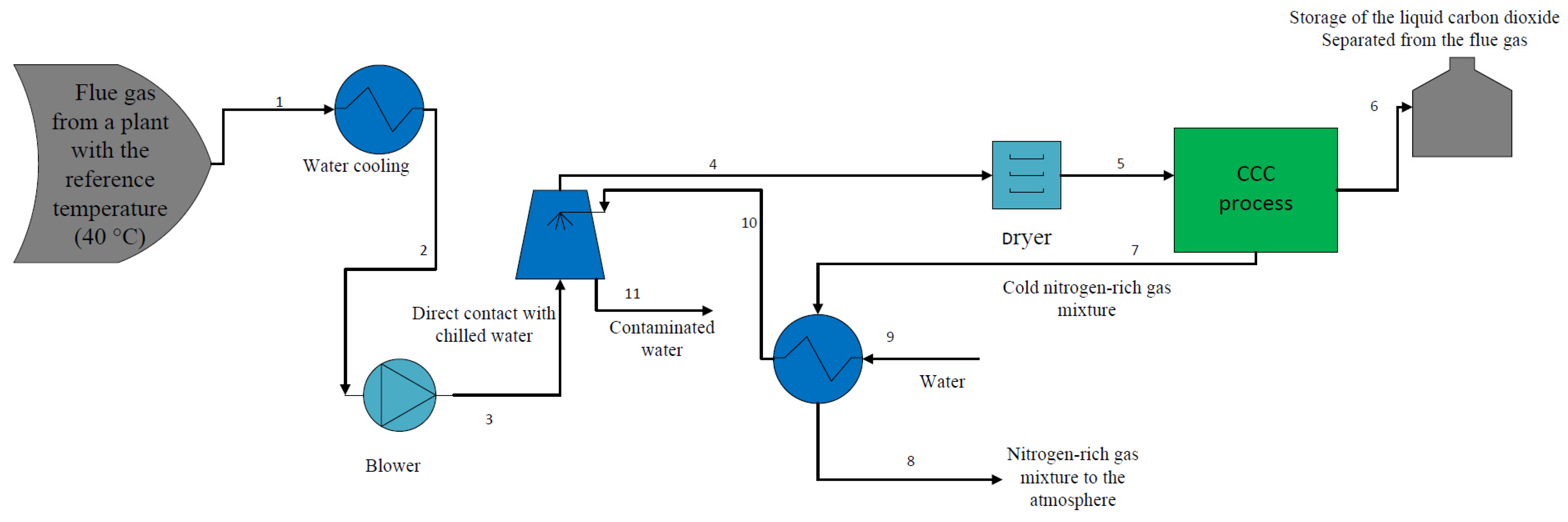
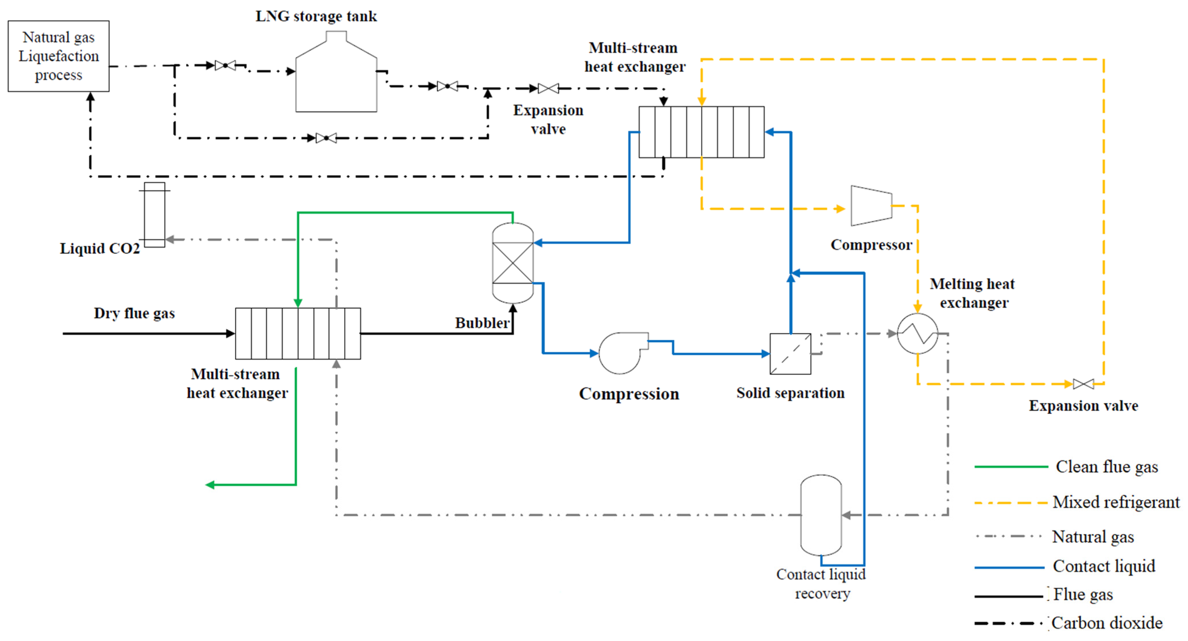
CCC Process Description

In this section, the pre-processing of the flue gas before entering the CCC process and the performance of the CCC process are concisely discussed. As Figure 1 indicates, the flue gas which leaves the plant should be cooled down to 40 °C (state 1) using a vapor compression refrigeration system or other methods (this temperature is considered as flue gas reference temperature for CO₂ capture processes according to NETL). Afterward, the flue gas temperature is further reduced by water cooling which results in reducing the flue gas temperature to 25 °C (state 2). The pressure of the flue gas is then increased to 1.4 bar using a blower (state 3). The flue gas is then cooled to 2 °C (state 4) and its hazardous components including mercury and sulfur dioxide will be washed away (state 11) as it comes to direct contact with chilled water at 1 °C (state 10) and it is directed to a dryer to remove its vapor content. Herein, the pre-processed flue gas (state 5) enters the CCC process to separate its CO₂ content. As a result, the separated CO₂ is stored in the form of liquid (state 6), while the cold nitrogen-rich gas mixture (state 7) might be used to generate chilled water before being released into the atmosphere (state 8).

The CCC process is shown in Figure 2. The process flow diagram shown by Figure 2 is similar to the process studied and evaluated by Jensen [8] and Fazlollahi et al. [23]. The dry flue gas after desulfurization enters the CCC process and it is cooled to 175 K by a nitrogen-rich gas mixture which comes from the desublimation heat exchanger and liquid CO₂ stream. Then, the flue gas enters a desublimation heat exchanger system, and its temperature is reduced to 154 K by contact liquid. As a result, the CO₂ in the flue gas undergoes a phase change and solid particles of CO₂ are formed. The clean flue gas leaves the desublimation heat exchanger system from the top and cools the incoming flue gas, while the CO₂/contact liquid slurry leaves the heat exchanger from the bottom and it is pressurized by a pump. The solid CO₂ particles are separated from the contact liquid by filtration. As Figure 2 indicates, the process requires two refrigeration loops termed the internal and external refrigeration cycles which have the highest energy consumption in the process. The internal refrigeration cycle which may use mixed refrigerant is responsible for providing a part of cooling energy that is used to cool down the contact liquid. As can be seen, the compressed mixed refrigerant is condensed by melting the solid CO₂ and increasing its temperature to 233 K. The liquid CO₂ stream flashes to generate pure liquid CO₂. The liquid-rich CO₂ stream cools the incoming flue gas before leaving the CCC process. The external refrigeration loop is also used to produce liquified natural gas to operate the process and provide the rest of the cooling effect for reducing the temperature of contact liquid. The C3MR natural gas liquefaction process is discussed in detail by Wang et al. [35]. The liquefied natural gas is used as an intermediate refrigerant to cool the contact liquid which is responsible for the desublimation of CO₂ in a heat exchanger. As shown in Figure 2, the LNG leaves the natural gas liquefaction process at a temperature of 179 K. When renewable energy is available and the energy price is low, extra LNG can be generated and stored in a tank. The stored LNG can be used during peak hours when the energy price is high. The LNG which comes from the tank/natural gas liquefaction process is expanded, and its temperature is reduced to 153.6 K; then, it enters a multi-stream heat exchanger to cool the contact liquid. The contact liquid is generally a hydrocarbon mixture, but it can be any other heat transfer fluid that has low viscosity and vapor pressure at cryogenic temperatures [8]. As shown in Figure 2, this liquid is used to separate CO₂ in a direct heat exchanger where it is mixed with the flue gases. Using a direct heat exchanger is operationally simple and can desublimate CO₂ continuously, while as Figure 2 indicates, a solid separation unit is required to separate solid particles of CO₂ from the liquid. In the case of using an indirect heat exchanger, the solid separation unit is not required. However, using this type of heat exchanger adds complexity to the process by causing challenges in cleaning the surface of heat exchangers, requiring maintenance cycles, and avoiding a continuous operation.

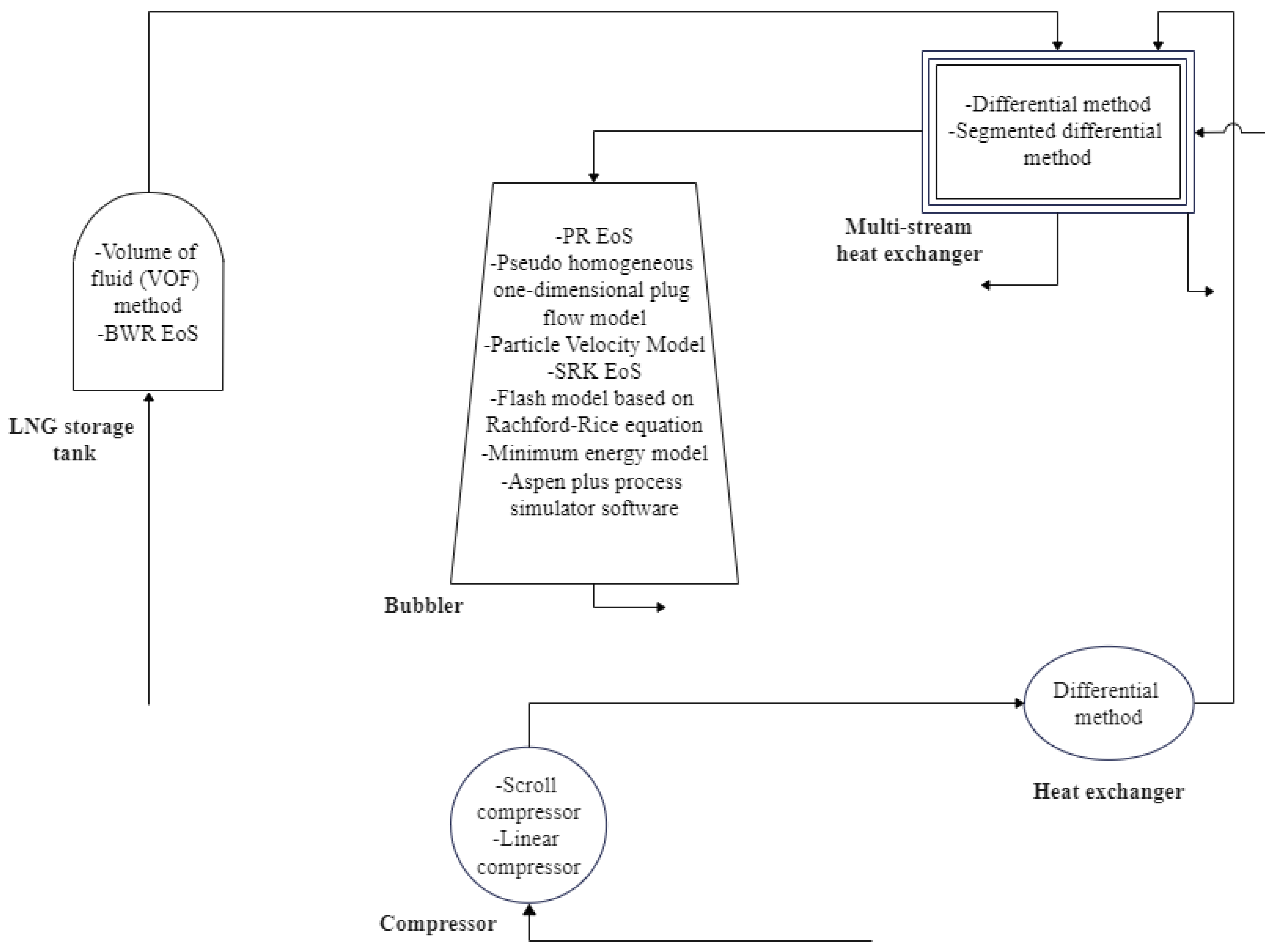
2. Modeling Approaches for the CCC Process

In this part, the most important models which are available in the literature and can be used to simulate the CCC process are discussed, and their advantage and accuracy are also evaluated. Figure 3 indicates different components and elements in the CCC process. The available methods which can be used to model and investigate each component are shown by this figure. In the figure, only the models that are deemed more effective for components modelling in the CCC processing are presented. In this section, a differential method for modeling the heat exchangers in the CCC process is discussed. This model can be used to simulate counter flow heat exchangers as well as multi-stream heat exchangers in the CCC process. Then, the particle velocity model and pseudo-homogeneous one-dimensional plug flow model, which can be used to study and model the desublimation heat exchanger in the CCC process, are presented. Furthermore, different equations which can be used to calculate the solid–vapor equilibrium and liquid–vapor equilibrium of CO₂ mixtures in the bubbler are presented in this section. These equations include PR EoS, the Rachford–Rice equation, and SRK EoS. The minimum energy model is also discussed in this section which can be used to calculate the minimum energy required for the separation of CO₂ from the flue gas using the CCC process under the ideal operating conditions. The volume of fluid and BWRS methods are also presented to model the LNG tank and calculate the boil-off-gas. Finally, the compression process model of scroll compressors and the linear compressor model are discussed to model the scroll compressors and the linear compressors, respectively.

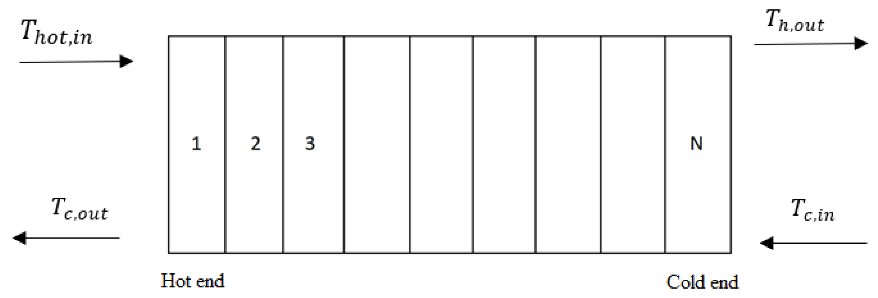
2.1. Heat Exchangers

As Figure 2 indicates, the CCC process deals with heat exchangers of different types. In this process and other cryogenic processes in general, plate-fin heat exchangers are widely used due to their exceptional advantages including compactness, low weight, and high efficiency. It is also worth noting that plate-fin heat exchangers are the only type of heat exchanger that can carry multiple streams [36]. Therefore, using an efficient, accurate, and fast method to model plate-fin heat exchangers are of paramount importance for modeling and investigating the CCC process. Different methods are available and can be used to simulate the heat exchangers. For instance, You et al. [37] developed a CFD method to model the shell and tube heat exchanger. They used porosity and permeability concepts in their model to reduce the computational costs. They modeled the heat exchanger over a wide range of Reynolds numbers, and they indicated that the model can predict the velocity and temperature fields with a maximum of 15% relative deviation. He et al. [38] also developed a modified porous medium model to evaluate flow characteristics and heat transfer on the shell side of shell and tube heat exchangers. They simulated three types of shell and tube heat exchangers with vertical baffles, helical baffles, and finned tube banks. Comparing the model results with experimental data showed that the model can predict a pressure drop with a maximum of 25.1% relative deviation. Haider et al. [39] also used Open-FOAM v6 to simulate a multi-stream plate-fin heat exchanger. In this study, they directly modeled and solved parting sheets and sidebars. However, to reduce computational costs and avoid the fine computational grid, the fins were not resolved directly. Therefore, they also used a porous medium approach and considered fins as porous solids. Korzeń et al. [40] also developed a mathematical model which can simulate the transient operation of a plate and fin heat exchanger to cool water with cold air. It can be used to model the transient response of the heat exchanger when the cold stream mass flow rate decreases suddenly and at the same time, the hot stream mass flow rate increases. Comparing the numerical results with experimental data showed that the model can predict the temperature of the outlet streams accurately.

In this part, a differential method for modeling heat exchangers in the CCC process is described and evaluated. This model can be used to simulate counter flow heat exchangers with acceptable accuracy and can also be extended to simulate multi-stream heat exchangers. Therefore, this method is advantageous, and because of that, it is discussed here.

Differential Method

The differential method is an accurate technique for modeling heat exchangers since, unlike the integral method which considers fixed values for thermo-hydraulic properties of hot and cold streams, this method considers the variation in thermo-hydraulic properties of process streams and integrates the heat transfer and pressure loss functions in a stepwise approach from one end to another end of heat exchangers. It has been shown that this method is very effective and efficient when the structure of the studied heat exchanger is very complex [41].

In the differential method, as shown in Figure 4, the length of the heat exchanger is divided into N sections where the thermo-hydraulic properties of streams are assumed to be invariant in each section. The temperature variation in the first section of the counter-flow heat exchanger for hot and cold streams can be calculated using the following equations [36]:

$$\mathsf{\Delta }{T}_{h,1}=\frac{\left(UA\right)\mathsf{\Delta }{T}_1}{N{C}_h}$$

(1)

$$\mathsf{\Delta }{T}_{c,1}=\frac{\left(UA\right)\mathsf{\Delta }{T}_1}{N{C}_c}$$

(2)

where (UA) is the overall heat transfer rate, while $C_c$ and $C_h$ represent the capacity rate of cold and hot streams, respectively, and $\mathsf{\Delta }{T}_1$ is the temperature difference between inlet hot and cold streams, which is always known. This value can be used to calculate the temperature difference at the starting point of the second partition, as follows:

$$\mathsf{\Delta }{T}_2=\mathsf{\Delta }{T}_1 [1-\frac{\left(UA\right)}{N}\left(\frac{1}{C_h}-\frac{1}{C_c}\right)]$$

(3)

Consequently, the temperature variation in the second section of the heat exchanger for hot and cold streams can be calculated using the following equations:

$$\mathsf{\Delta }{T}_{h,2}=\frac{\left(UA\right)\mathsf{\Delta }{T}_1}{N{C}_h} [1-\frac{\left(UA\right)}{N}\left(\frac{1}{C_h}-\frac{1}{C_c}\right)]$$

(4)

$$\mathsf{\Delta }{T}_{c,2}=\frac{\left(UA\right)\mathsf{\Delta }{T}_1}{N{C}_c} [1-\frac{\left(UA\right)}{N}\left(\frac{1}{C_h}-\frac{1}{C_c}\right)]$$

(5)

Therefore, temperature variations for hot and cold streams in the third partition of the heat exchanger can be found by multiplying Equations (4) and (5) by the second term on the right side of Equation (3). Under this situation, temperature variation in the last partition for hot and cold streams can be calculated using the following equations:

$$\mathsf{\Delta }{T}_{h,N}=\frac{\left(UA\right)\mathsf{\Delta }{T}_1}{N{C}_h} {[1-\frac{\left(UA\right)}{N}\left(\frac{1}{C_h}-\frac{1}{C_c}\right)]}^{N-1}$$

(6)

$$\mathsf{\Delta }{T}_{c,N}=\frac{\left(UA\right)\mathsf{\Delta }{T}_1}{N{C}_c} {[1-\frac{\left(UA\right)}{N}\left(\frac{1}{C_h}-\frac{1}{C_c}\right)]}^{N-1}$$

(7)

The temperature difference between hot and cold streams at the cold end of the heat exchanger can also be obtained using the following equation:

$$\mathsf{\Delta }{T}_{N+1}=\mathsf{\Delta }{T}_{ce}=\mathsf{\Delta }{T}_1 {[1-\frac{\left(UA\right)}{N}\left(\frac{1}{C_h}-\frac{1}{C_c}\right)]}^N$$

(8)

where $\mathsf{\Delta }{T}_{ce}$ is the temperature difference between hot and cold streams at the cold end of the counter flow heat exchanger which is the right wall of section N in Figure 4. At this point, the temperature distribution of cold and hot streams along a counter-flow heat exchanger can be obtained using Equations (1)–(8), having the inlet temperature of hot and cold streams.

Considering Equations (1)–(8), temperature variation sets along the heat exchanger forms a geometric series. Therefore, summation of the series and letting N tend to infinity generates the following equations:

$$T_{h,in}-T_{h,out}=\frac{C_c\mathsf{\Delta }{T}_{he}}{C_c-C_h}(1-e^{UA(\frac{1}{C_c}-\frac{1}{C_h})})$$

(9)

$$T_{c,out}-T_{h,in}=\frac{C_c\mathsf{\Delta }{T}_{he}}{C_c-C_h}(1-e^{UA(\frac{1}{C_c}-\frac{1}{C_h})})$$

(10)

$$\mathsf{\Delta }{T}_{ce}=\mathsf{\Delta }{T}_{he}{e}^{UA\left(\frac{1}{C_c}-\frac{1}{C_h}\right)}$$

(11)

In the case of using multi-stream heat exchangers, Equations (9)–(11) can be extended in the following forms to calculate the temperature difference between hot and cold streams in both hot and cold ends:

$$\mathsf{\Delta }{T}_{he}=\frac{{\sum }_{i=1}^{nh}{h}_i{A}_i{T}_{in,i}}{{{\displaystyle \sum }}_{i=1}^{nh}{h}_i{A}_i}-\frac{{{\displaystyle \sum }}_{i=1}^{nc}{h}_i{A}_i{T}_{out,i}}{{{\displaystyle \sum }}_{i=1}^{nc}{h}_i{A}_i}$$

(12)

$$\mathsf{\Delta }{T}_{ce}=\frac{{{\displaystyle \sum }}_{i=1}^{nh}{h}_i{A}_i{T}_{out,i}}{{{\displaystyle \sum }}_{i=1}^{nh}{h}_i{A}_i}-\frac{{{\displaystyle \sum }}_{i=1}^{nc}{h}_i{A}_i{T}_{in,i}}{{{\displaystyle \sum }}_{i=1}^{nc}{h}_i{A}_i}$$

(13)

where nc and nh denote the number of cold and hot streams, respectively, while $h_i$ and $A_i$ are the heat transfer coefficient and net effective surface area of the stream $i$, respectively.

The surface temperature of a multi-stream heat exchanger can also be calculated using the following equation:

$$T_s=\frac{{{\displaystyle \sum }}_{i=1}^{nh}{h}_i{A}_i{T}_i+{{\displaystyle \sum }}_{i=1}^{nc}{h}_i{A}_i{T}_i}{{{\displaystyle \sum }}_{i=1}^{nh}{h}_i{A}_i+{{\displaystyle \sum }}_{i=1}^{nc}{h}_i{A}_i}$$

(14)

As Equation (14) indicates, it is assumed that the surface temperature of the heat exchanger in all cross sections has a constant value. This assumption brings about significant simplicity in calculations by limiting the unknown parameters to stream temperatures and surface temperature. It is also worth noting that when a satisfactory stacking pattern is used, especially in multi-stream heat exchangers, the model which uses this assumption can predict temperature with very low errors [39,40].

The differential method is discussed in more detail in [36,42] by providing and designing a computer program for evaluating the performance of a counter flow heat exchanger.

Wang et al. [38] developed a novel segmented differential method to model and optimize a multi-stream compact heat exchanger. In this method, a multi-stream compact heat exchanger is fragmented into several sections along the direction of the mainstream. Each section is considered as a sub-heat exchanger which is made of N layers and N − 1 separating plates along the height of the heat exchanger. This model is developed to determine the temperature and pressure of streams along with the temperature of separating plates at each computational node. Therefore, heat transfer equations along with energy conservation equations in the entire computational domain of a sub-heat exchanger should be solved to calculate the unknown parameters. The calculated parameters are then used as inputs for the next sub-heat exchanger. The energy conservation for streams is presented by the following equation [41]:

$$D{F}_i\frac{d{T}_i}{dx}=\left(1-{\omega }_i{\delta }_i\right)h_i[T_{p,i}\left(x,0\right)+T_{p,i}\left(x,b_i\right)-2T_i\left(x\right)]+2{\omega }_i{h}_i{{\displaystyle \int }}_0^{bi} [T_{f,i}\left(x,y\right)-T_i\left(x\right)]dy$$

(15)

On the left side of Equation (15), the energy gradient at $i^{\mathrm{th}}$ node is indicated where D represents the sign symbol of flow direction while T and F are the stream temperature and heat capacity flow rate, respectively. On the right side of this equation, however, convective heat transfer on the separating plates and fins is provided where $\omega$, $\delta$, $b$, and $h$ stand for fin number per unit width, fin thickness, fin height, and convective heat transfer coefficient, respectively. Subscriptions $p$, $f$, and $i$ also indicate separating plate, fin, and the number of nodes, respectively.

Energy conservation for separating plates can also be presented by the following equation:

$$\begin{array}{l}{\omega }_{i+1}{\delta }_{i+1}\lambda \frac{\partial T_{p,i+1}\left(x,y\right)}{\partial \mathrm{y}}\left(y=0\right)-{\omega }_i{\delta }_i\lambda \frac{\partial T_{p,i}\left(x,y\right)}{\partial \mathrm{y}}\left(y=b_i\right)+{\delta }_i\lambda \frac{{\partial }^2{T}_{p,i}}{\partial x^2}\\ \hspace{1em}\hspace{1em}\hspace{1em}=\left({\omega }_i{\delta }_i-1\right)h_i[T_i\left(x\right)-T_{p,i}\left(x,b_i\right)]+\left({\omega }_{i+1}{\delta }_{i+1}-1\right)h_{i+1}[T_{i+1}\left(x\right)-T_{p,i+1}\left(x,0\right)]\end{array}$$

(16)

where $\lambda$ represents thermal conductivity.

Finally, energy conservation for fins is given by making a balance between the convective heat transfer rate (the left side of equation) and conduction heat transfer rate (the right side of the equation), as follows:

$$2{\omega }_i{h}_i[T_{f,i}\left(x,y\right)-T_i\left(x\right)]={\omega }_i{\delta }_i\lambda [\frac{{\partial }^2{T}_{f,i}\left(x,y\right)}{\partial x^2}+\frac{{\partial }^2{T}_{f,i}\left(x,y\right)}{\partial y^2}]$$

(17)

The differential method is an accurate model which can precisely determine the variation in the temperature and pressure field inside the heat exchanger [42]. However, this model has a higher computational cost when it is compared with the integral method, especially when it is used for dynamic models. Therefore, the integral method would be more applicable for dynamic applications when the internal pressure and temperature fields are not required.

2.2. Bubbler (CO₂ Separator)

In this part, the available models and equations of states which can be used to model the desublimation heat exchangers and packed beds in the CCC process and calculate the solid–vapor equilibrium and liquid–vapor equilibrium are given. In the analyzed studies, the models and equations of states which have mainly been considered for their accuracy and computational effectiveness can be listed as:

• Particle velocity model;
• Pseudo homogeneous one-dimensional plug flow model;
• Peng Robinson EoS;
• Flash model based on the Rachford–Rice equation.

The last model has been used to calculate the solid–vapor equilibrium temperature by Guido et al. [43]. However, in this study, it is extended to calculate the liquid–vapor equilibrium. The model’s accuracy compared to the experimental value will be later provided in

Table A1. The Available Methods and Their Accuracy for Modeling Different Components in the CCC Process.

Simulation Method	AAD% 1	Application	Reference Number
1D model using particle velocity method	4% [44]	Simulation of desublimation exchanger system	[44]
ASPEN Plus (version 7.3)	-	Modeling the overall energy consumption in the CCC process based on Stirling cooler	[17]
A steady state model using ASPEN Plus	6.6%	Simulation of the CCC process using energy storage system	[8]
A steady state model using ASPEN Plus	1% [22]	Modeling the energy consumption in the process and sizing the required heat exchangers	[22]
1-D pseudo homogeneous axially dispersed plug flow model	2.2%	Dynamic simulation of packed beds used in the CCC process.	[46,47]
ASPEN HYSYS commercial process simulator	-	Modeling four different natural gas liquefaction processes to supply the required LNG in the CCC process	[23]
ASPEN HYSYS commercial process simulator and exergy analysis		Modeling a small-scale natural gas liquefaction process	[24]
Differential method	-	3D simulation of multi-stream heat exchangers	[36]
A 3D model based on segmented differential method	-	Modeling multi-stream heat exchangers	[41]
Differential method	-	Modeling and sizing multi-stream heat exchangers	[42]
A 2D model using VOF method and ANSYS FLUENT commercial process simulator	6.5% [71]	Modeling large-scale LNG storage and carbon capture systems	[71]
BWRS EoS model	-	Modeling BOG generation in LNG tanks	[72]
A 2D model using VOF method and ANSYS FLUENT commercial process simulator	4% [78]	Modeling the evaporation and condensation phase-change processes	[78]
A 3D model using Eulerian multiphase flow method and ANSYS FLUENT commercial process simulator 6.2	-	Modeling refrigerant flow boiling in horizontal serpentine tube	[79]
A 2D model using VOF method and ANSYS FLUENT commercial software, version 19	-	Simulation of natural convection and BOG generation in small, pressurized LNG storage tank	[84]
A 3D model using VOF method and ANSYS FLUENT commercial process simulator	10% [85]	Simulation of BOG generation rate for LNG tank	[85]
A 2D model using VOF method and ANSYS FLUENT commercial process simulator	5% [86]	Simulation of BOG generation rate for LNG tank	[86]
Compression Process Model	-	Modeling scroll compressors which can be used in the CCC process	[90]
An improved BWRS EoS model	0.35% [88]	Predicting thermodynamic properties at extreme low reduced temperature	[88]
Modified SRK EoS model	1% [63]	Predicting the vapor–liquid equilibrium in binary asymmetric mixtures	[63]
Minimum energy model	-	Minimum energy required for separating CO2 from the flue gas	[59]
Classical approach based on PR EoS model and ASPEN Plus commercial process simulator V9	1.4% for classical approach 2.9% for ASPEN Plus commercial process simulator V9	Predicting solid–vapor equilibrium conditions and specifying suitable operating conditions for capturing CO2 from the exhaust gases based on the required CO2 recovery level	[65]
Thermodynamic model and ASPEN Plus commercial process simulator V9	1.364% for the thermodynamic model 1.293% for ASPEN Plus commercial process simulator V9 [66]	Predicting multi-phase equilibrium conditions of CO2 mixtures with hydrocarbon and non-hydrocarbon components and presenting stability analysis	[66]
ASPEN Plus commercial process simulator	4.31% [64]	Simulation and economic analysis of a cryogenic carbon capture process assisted by a solar absorption refrigeration system	[64]
Rachford–Rice flash model	1.27% in the pressure range of 1–15 bar	SVE calculation and predicting the frost point temperature of CO2	[43]
Linear compressor	2.47% and 8.49% for prediction of mass and power [93]	Modeling two-stage linear compressor	[93]
ASPEN Plus	-	SVE calculations for CO2 capture application	[96]
ASPEN HYSIS	-	Modeling and evaluation of a combined system of steam methanol reforming/steam methane reforming/high temperature PEM fuel cells/CO2 capture/liquefaction	[97]
ASPEN HYSIS	-	Process design and thermoeconomic evaluation of a CO2 liquefaction process (Energy, exergy, and exergoeconomic analyses)	[98]
Transient model using ASPEN HYSIS and PR EoS	-	Modeling and optimizing natural gas liquefaction process which provides coolant for CCC process	[99]
Aspen plus model using SRK	-	Modeling hybrid membrane-cryogenic capture process	[100]

¹ ($\mathrm{ADD}\%=\frac{{{\displaystyle \sum }}_{i=1}^{number of points}\frac{\left|variabl{e}_{cal,i}-variabl{e}_{exp,i}\right|}{variabl{e}_{exp,i}}}{number points }\times 100$).

.

In this part, the particle velocity model and pseudo homogeneous one-dimensional plug flow model are discussed first, and reference to the relevant studies is provided. These two models can be used to study, investigate, and simulate the desublimation heat exchanger system and packed beds in the CCC process. Then, the equations used to perform the phase equilibrium analysis of CO₂ mixtures at cryogenic temperatures are given.

2.2.1. Particle Velocity Model

The desublimation process in the bubbler shown in Figure 2 is simulated by James et al. [44] using the particle velocity method. This model was applied to simulate the phase change processes including the desublimation of CO₂. Therefore, this model solves heat and mass transfer equations simultaneously along with the momentum transfer equation to track the phase changes.

A one-dimensional numerical model of the desublimation heat exchanger system is used to predict temperature distribution, velocity, pressure, composition, mass, and heat transfer rates inside the heat exchanger. It was assumed that the local solid–vapor equilibrium exists in the particle interface and these particles are distributed uniformly inside the heat exchanger and are displaced equally. The CO₂-rich flue gas stream enters the bottom of the heat exchanger. In this case, as discussed before, a cool exchange medium enters the top of the heat exchanger and cools the flue gas from −98 °C to very low temperatures (−138 °C) [44]. Therefore, CO₂ is separated from the flue gas in the form of solid particles. As a result, the CO₂/exchange liquid slurry leaves the bottom of the heat exchanger, while CO₂ lean gas leaves the top of the heat exchanger.

In this model, the following equation is used to describe convection heat transfer from or to droplets.

$$q=ANh\theta \left(T_s-T_g\right)$$

(18)

where A, N, h, and $\theta$ represent the droplet surface area, the number of solid particles, convective heat transfer coefficient, and blowing factor, respectively. It is assumed that droplets have a constant surface temperature and composition. The convective heat transfer coefficient is given as follows:

$$h=\frac{Nu{d}_p}{k}$$

(19)

where k, $d_p$, and Nu represent the conductive heat transfer coefficient, particle diameter, and Nusselt number, respectively. The latter parameter can be calculated using the following equation:

$$Nu=2+0.6R{e}^{0.5}P{r}^{\raisebox{1ex}{$1$}\!\left/ \!\raisebox{-1ex}{$3$}\right.}$$

(20)

The rate of evaporation and desublimation can also be calculated using the following equation:

$$W_{A0,i}=\frac{k_{xm}{\theta }_m\pi d_p{}^{2}N\frac{P_{vap}}{P_{tot}}-x_{A\infty }+W_{B0,i}\frac{P_{vap}}{P_{tot}}}{1-\frac{P_{vap}}{P_{tot}}}$$

(21)

where $x_{A\infty }$ and $W_{B0,i}$ represent the mole fraction of CO₂ in upstream flow and the rate of evaporation, respectively. $P_{vap}$ and $k_{xm}$ are also vapor pressure and mass transfer coefficient, respectively, which are given as follows [44,45]:

$$P_{vap}=\exp (A+\frac{B}{T}+Cln\left(T\right)+D{T}^E)$$

(22)

$$k_{xm}=\frac{Sh{d}_p}{D_{AB}}$$

(23)

where $D_{AB}$ is binary diffusivity and $Sh$ is the Sherwood number, which can be calculated as follows:

$$Sh=2+0.6R{e}^{0.5}S{c}^{\raisebox{1ex}{$1$}\!\left/ \!\raisebox{-1ex}{$3$}\right.}$$

(24)

where $Sc$ denotes the Schmidt number, which is defined using the following equation:

$$Sc=\frac{\upsilon }{D_{AB}}$$

(25)

The particle velocity model represented here can be effectively used to study and evaluate the motion of solid CO₂ particles inside the heat exchanger and to determine their velocity. Therefore, the model considers the main forces including buoyancy and drag which affect the particles and can be calculated as follows:

$$F_b={\rho }_g-{\rho }_p\frac{\pi d_p{}^{3}g}{6}$$

(26)

$$F_d=\frac{C_D}{8}{\rho }_g{\upsilon }_{rel}{}^2\pi d_p{}^2$$

(27)

where $F_b$, $F_d$, $C_D$, and ${\upsilon }_{rel}$ are buoyancy force, drag force, drag coefficient, and velocity of particle relative to the cool exchange medium, respectively, while $g$ and $p$ subscriptions represent the gas phase and solid phase for particles, respectively. Moreover, g stands for gravity and possesses a negative value in Equation (26), and the direction of drag force is also in the opposite direction of particle relative velocity. Therefore, considering Equations (26) and (27), the overall force applied to particle $i$ can be calculated as follows:

$$F_i={\rho }_g-{\rho }_p\frac{\pi d_p{}^{3}g}{6}+\frac{C_D}{8}{\rho }_g{\upsilon }_{rel}{}^2\pi d_p{}^2$$

(28)

Considering Equation (28) and Newton’s third law, the velocity of particle $i$ is given as follows:

$${\upsilon }_{p,i}=\frac{F_i}{m_p}dt+{\upsilon }_{p,i-1}$$

(29)

where $m_p$ indicates the mass of particle. It should be noted that the velocity of particles calculated using Equation (29) cannot exceed terminal velocity which is defined as the highest velocity limit which a particle can approach. Therefore, when a particle reaches this velocity, it neither accelerates nor decelerates. The value of terminal velocity can be calculated by assigning a zero value for overall force in Equation (28) and solving the equation for the velocity.

This model which considers different heat and mass transfer relationships can be used to investigate, optimize, and simulate the desublimation heat exchanger system which is made of vertical countercurrent heat exchangers. This heat exchanger system can be used to cool down the rich CO₂ flue gas from −98 to −138 °C where the pressure may vary from ambient pressure to several bars. To model this heat exchanger system, momentum, species continuity, and energy equations are solved at the same time for both solid and gas phases in a one-dimensional heat exchanger which operates under steady-state conditions.

2.2.2. Pseudo-Homogeneous One-Dimensional Plug Flow Model

This model is applied to study the dynamic behavior of packed beds used in the CCC process [46,47]. In this case, flue gas, which is composed of N₂, CO₂, and H₂O at a comparatively high temperature is fed to an initially refrigerated packed bed which results in the separation of the components since they have different dew and sublimation points. The separation process consists of three steps including the capture cycle, CO₂ recovery cycle, and cooling cycle. These three cycles are discussed in detail in reference [47]. The process for capturing CO₂ can be simulated using a Pseudo homogeneous one-dimensional plug flow. To simulate the process, component mass balances for the gaseous phase are given as follows [47]:

$${Є}_g{\rho }_g\frac{\partial {\omega }_{i,g}}{\partial t}=-{\rho }_g{\upsilon }_g\frac{\partial {\omega }_{i,g}}{\partial z}+\frac{\partial }{\partial z}({\rho }_g{D}_{eff}\frac{\partial {\omega }_{i,g}}{\partial z})-{\dot{m}}_i^{″}{a}_s+{\omega }_{i,g}{{\displaystyle \sum }}_{i=1}^{n_c}{\dot{m}}_i^{″}{a}_s$$

(30)

where ${Є}_g$, ${\omega }_{i,g}$, ${\upsilon }_g$, $D_{eff}$, $a_s$, z, and ${\dot{m}}_i^{″}$ represent bed void fraction, mass fraction of $i^{th}$ gaseous component, superficial velocity, effective diffusion coefficient, specific solid surface area per unit bed volume, the axial coordinate of the bed, and mass deposition rate per unit surface area for component i, respectively.

The following equation also provides component mass balance for the solid phase:

$$\frac{\partial m_i}{\partial t}={\dot{m}}_i^{″}{a}_s$$

(31)

where $m_i$ denotes the mass deposition of component i per unit volume of the bed.

The total continuity equation for the gaseous phase is given as follows:

$$\frac{\partial \left({Є}_g{\rho }_g\right)}{\partial t}=-\frac{\partial \left({\rho }_g{\upsilon }_g\right)}{\partial z}-{{\displaystyle \sum }}_{i=1}^{n_c}{\dot{m}}_i^{″}{a}_s$$

(32)

In this model, the energy balance for gas and solid phases is given as follows:

$$({Є}_g{\rho }_g{C}_{p,g}+{\rho }_s\left(1-{Є}_g\right)C_{p,s})\frac{\partial T}{\partial t}=-{\rho }_g{\upsilon }_g{C}_{p,g}\frac{\partial T}{\partial z}+\frac{\partial }{\partial z}({\lambda }_{eff}\frac{\partial T}{\partial z})-{{\displaystyle \sum }}_{i=1}^{n_c}{\dot{m}}_i^{″}{a}_s\mathsf{\Delta }{h}_i$$

(33)

where $C_{p,s}$ and $C_{p,g}$ represent the specific heat for solid and gas phases, respectively, while $\mathsf{\Delta }{h}_i$ and ${\lambda }_{eff}$ are enthalpy change due to phase change of component i and effective conductivity, respectively. The latter parameter can be calculated as follows:

$${\lambda }_{eff}={\lambda }_{bed, 0}+\frac{RePr{\lambda }_g}{P{e}_{ax}}+\frac{R{e}^{2}P{r}^2{\lambda }_g}{6\left(1-{Є}_g\right)Nu}$$

(34)

where ${\lambda }_{bed, 0}$ is the effective bed conductivity at no flow condition, while $P{e}_{ax}$ is the Peclet number for axial heat dispersion and can be calculated as follows:

$$P{e}_{ax}=\frac{2p}{1-p}$$

(35)

where p is defined as follows:

$$p=0.17+0.33ex{p}^{\frac{-24}{Re}}$$

(36)

Nusselt number can be calculated to obtain gas-to-particle heat transfer coefficient as follows:

$$Nu=\left(7-10{Є}_g+5{Є}_g{}^2\right)\left(1+0.7R{e}^{0.2}P{r}^{\raisebox{1ex}{$1$}\!\left/ \!\raisebox{-1ex}{$3$}\right.}\right)+\left(1.33-2.4{Є}_g+1.2{Є}_g{}^2\right)R{e}^{0.7}P{r}^{\raisebox{1ex}{$1$}\!\left/ \!\raisebox{-1ex}{$3$}\right.}$$

(37)

Axial mass dispersion can also be calculated as follows:

$$\frac{D_{eff}}{d_p{\upsilon }_g}=\frac{0.73}{ReSc}+\frac{0.5}{{Є}_g [1+(\frac{9.7{Є}_g}{ReSc})]}$$

(38)

Mass deposition/condensation and evaporation parameters used in Equations (30)–(33) are given in the following equation:

$${\dot{m}}_i^{″}=\{\begin{array}{c}g\left(y_{i,s}p-p_i^{\sigma }\right) if y_{i,s}\ge p_i^{\sigma }\\ g\left(y_{i,s}p-p_i^{\sigma }\right)\frac{m_i}{m_i+o.1 } if y_{i,s}<p_i^{\sigma }\end{array}$$

(39)

where $y_{i,s}$ and g represent the molar fraction of component ith in solid phase and mass deposition rate constant, respectively, while $\sigma$ superscript indicates the equilibrium condition. To calculate the axial temperature and mass deposition profiles, the partial differential equations given by Equations (30)–(33) can be converted to ordinary differential equations using the method of lines (MOL). The utilization and implementation of this method are discussed in reference [48]. The resulting system of ordinary differential equations can be solved by ODE solvers such as ODE 15 s, which are available in MATLAB^®. Furthermore, the above-mentioned one-dimensional convection-dominated PDEs can also be solved using a numerical algorithm based on WENO principles by considering a higher-order discretization for the convection terms and automatic local grid adaptation. More details about the numerical algorithm can be found in Smit et al. [49].

2.2.3. Peng Robinson

Peng Robinson Equation of State (PR EoS) is one of the most popular and accurate applied models for thermodynamic and volumetric calculations since 1976 and can be used to obtain thermo-physical and phase equilibrium properties of CO₂. The most convenient form of PR EoS is given by the following equation:

$$p=\frac{RT}{\upsilon -b}-\frac{a}{\upsilon \left(\upsilon +b\right)+b\left(\upsilon -b\right)}$$

(40)

where T, $\upsilon$, and p represent temperature, specific volume, and pressure, respectively, while a and b are empirical parameters. These two parameters are used to consider the effect of attraction forces between the molecules and the molecular volume. For pure material, they can be calculated as follows [50]:

$$a=0.45724\frac{R^2{T}_c^2}{P_c} [1+m{(1-{(\frac{T}{T_c})}^{0.5})}^2$$

(41)

$$b=0.0778\frac{R{T}_c}{P_c}$$

(42)

$$m=0.37464+1.5422\omega -0.2699{\omega }^2$$

(43)

where $T_c$, $P_c$, and $\omega$ represent critical temperature, critical pressure, and acentric factor, respectively. This model has been applied, investigated, and modified by numerous researchers and more than 220 modifications have been reported for this model which can be found in a paper published by Lopez-Echeverry et al. [51]. Although in many cases the modifications applied to PR EoS follow the same ideas, differences in details are substantial, and because of that, each version generates a definite improvement compared to other versions of the model [52]. PR EoS can be used to calculate the fugacity coefficient of components in a mixture that is involved in the equilibrium condition to predict the solid–vapor or liquid–vapor equilibrium temperature. Therefore, to apply the PR EoS represented by Equations (40)–(43), it is necessary to use mixing rules to calculate parameters a and b. There are several mixing rules available including Wong–Sandler (WS) and Modified Huron–Vidal second-order model (MHV2), and they are discussed by Yang et al. [53]. Here, the Vander Waals (vdW) mixing rule is discussed and used to calculate a and b parameters in a mixture, as follows [53]:

$$a_m={{\displaystyle \sum }}_i^{NC}{{\displaystyle \sum }}_j^{NC}{x}_i{x}_j\left(1-k_{ij}\right){\left(a_i{a}_j\right)}^{0.5}$$

(44)

$$b_m={{\displaystyle \sum }}_i^{NC}{x}_i{b}_i$$

(45)

where NC and x stand for the number of components in the mixture and mole fraction, respectively, and the value of $a_i$ and $b_i$ can be calculated using Equations (41) and (42). $k_{ij}$ also represents the binary interaction parameter between i and j species. This parameter can be calculated as a function of temperature by minimizing the difference between experimental and calculated freezing temperature as discussed by reference [54]. It is also worth noting that ASPEN Plus^® V9.0 (AspenTech [55]) can also be used to obtain this parameter. Once the empirical parameters are calculated using Equations (44) and (45), the following equation can be applied to obtain the fugacity coefficient of a specific component in the mixture [53]:

$${\phi }_i\left(T,P,x_i\right)=\exp \{\left(\frac{b_i}{b}\right)\left(z-1\right)-\ln \left(z-B\right)-\frac{A}{2.828B}\left(\frac{2{{\displaystyle \sum }}_j^{NC}{x}_j{\left(a_i{a}_j\right)}^{0.5}\left(1-k_{ij}\right)}{a}-\frac{b_i}{b}\right)\ln (\frac{z+2.414B}{z-0.414B})\}$$

(46)

$$A=\frac{ap}{R^2{T}^2}$$

(47)

$$B=\frac{bp}{RT}$$

(48)

where z in Equation (46) represents the compressibility factor. Equation (49) represents the solid–vapor equilibrium and can be used to calculate the freezing point of CO₂ [54]:

$$y_{C{O}_2}{\phi }_{C{O}_2}^{V}P-P_{C{O}_{2}Solid}^{Sat}{\phi }_{C{O}_2}^{Sat}\exp [\frac{v_{C{O}_{2}Solid}}{RT}\left(P-P_{C{O}_{2}Solid}^{Sat}\right)]=0$$

(49)

where $y_{C{O}_2}$, ${\phi }_{C{O}_2}^V$, P, $P_{C{O}_{2}Solid}^{Sat}$, ${\phi }_{C{O}_2}^{Sat}$, and $v_{C{O}_{2}Solid}$ are the mole fraction of CO₂ in the vapor phase, the vapor phase partial fugacity coefficient for CO₂, the system pressure, solid CO₂ vapor pressure, the fugacity of pure CO₂ vapor at $P_{C{O}_{2}Solid}^{Sat}$, and the molar volume of solid CO₂, respectively. However, in the case of liquefying CO₂ and separating it from the gas mixture, the following VLE relationship can be used to calculate the dew point of CO₂ [56]:

$$y_{C{O}_2}{\phi }_{C{O}_2}^V=x_{C{O}_2}{\phi }_{C{O}_2}^l$$

(50)

where $y_{C{O}_2}$ and $x_{C{O}_2}$ represent the mole fraction of CO₂ in vapor and liquid phases, respectively. It has been reported that the PR EoS is more accurate than SRK (Soave—Redlich-Kwong) and RK (Redlich–Kwong) equations of states and the calculated results fit the experimental data with higher accuracy [53]. However, the accuracy of this model decreases as the pressure increases.

As discussed above, PR EoS or other equations of state such as SRK EoS along with a mixing rule are mostly used to calculate the solid–vapor equilibrium and liquid–vapor equilibrium of CO₂ mixtures. In other words, the equation of state and the selected mixing rule are used together in order to perform the phase equilibrium analysis of CO₂ in a gas mixture and predict the CO₂ dew point and freezing point.

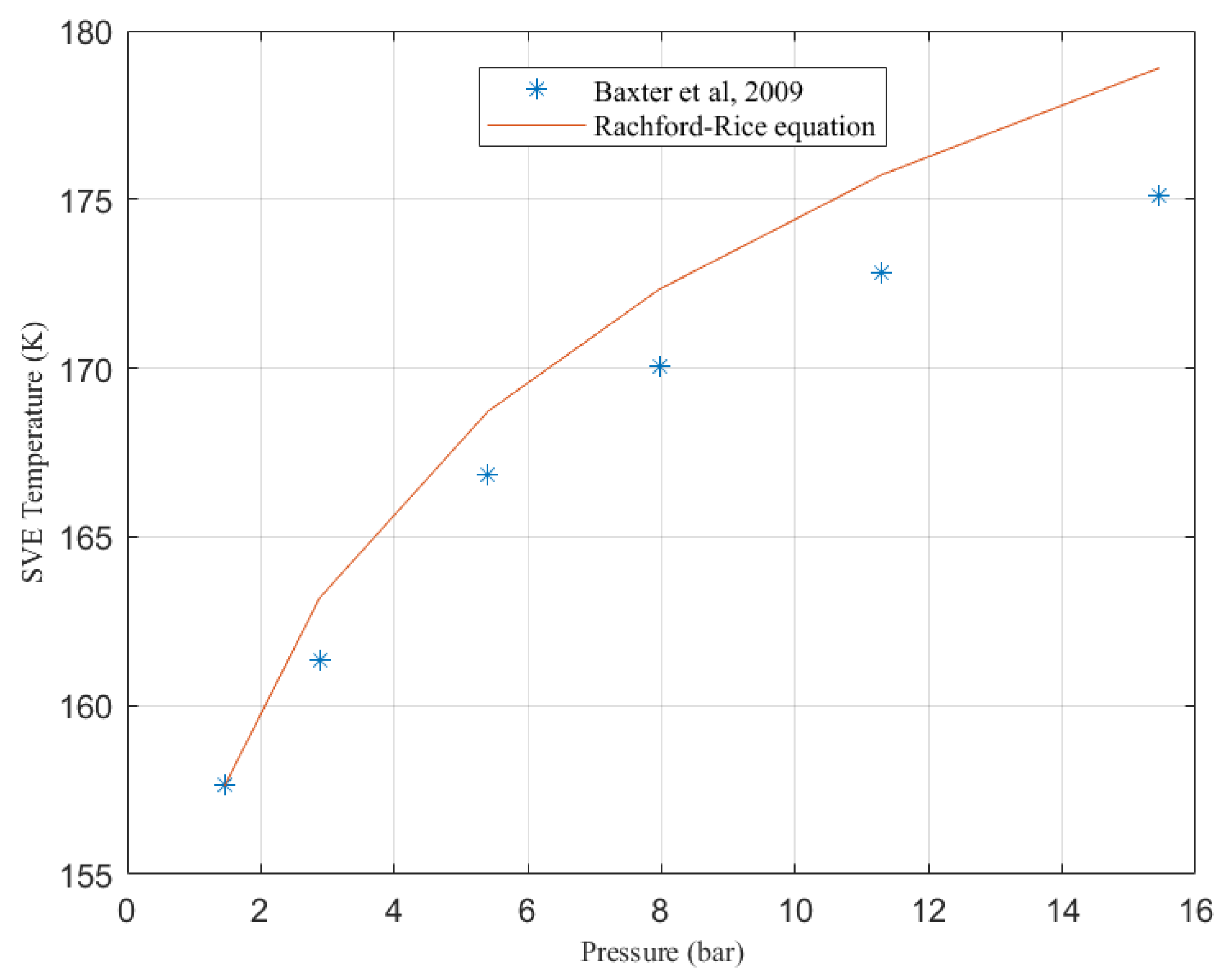
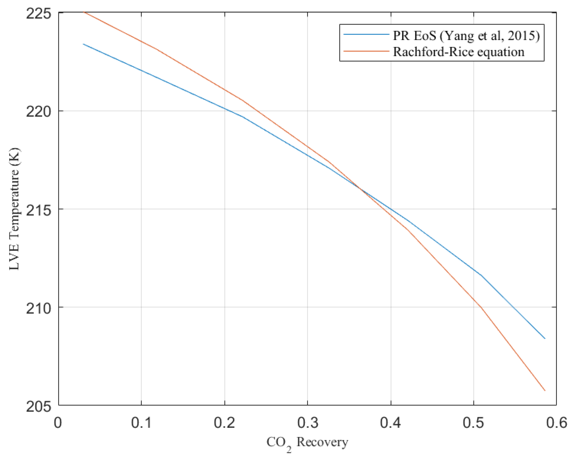
2.2.4. Flash Model Based on the Rachford–Rice Equation

The Rachford–Rice equation, which is mostly used for the flash calculation, can be used to model SVE conditions and the separation of CO₂ from a gas mixture in the solid form. In this case, the feed gas with a molar flow rate of F and composition of z which may contain N₂, O₂, and CO₂ enters a flash tank. As a result, solidified CO₂ with a molar flow rate of S leaves the tank from the bottom, while uncondensed gases with a molar flow rate of V and composition of x^V leave the tank from the top. The CO₂ recovery for the separation process can be defined as follows when it is assumed that pure CO₂ is formed in the solid phase [43]:

$$Rec=\frac{S}{F{z}_{C{O}_2}}$$

(51)

The following equations can also be used to discuss the mass balance in the separation process [43]:

V = F − S

(52)

$$V{x}_i^V=F{z}_i (\mathrm{if} i \ne {\mathrm{CO}}_2)$$

(53)

$$V{x}_{C{O}_2}^V=(1-REC) F{z}_{C{O}_2}$$

(54)

The Rachford–Rice equation, which is used for the SVE calculation, is given as follows:

$${{\displaystyle \sum }}_{i=1}^{NC}\frac{z_i\left(K_i-1\right)}{1+\frac{V}{F}\left(K_i-1\right)}=0$$

(55)

where $z_i$ and $K_i$represent the mole fraction and equilibrium constant of i-th component in the feed gas. The latter parameter can be calculated as follows:

$$K_i = \frac{x_i^V}{x_i^S}$$

(56)

As mentioned before, only CO₂ will be formed in the solid phase and because of that the equilibrium constant for other components rather than CO₂ would reach infinity. Under this situation, considering Raoult’s law, the equilibrium constant for CO₂ can be calculated by the following equation:

$$K_{{\mathrm{CO}}_2}=\frac{P_{sub}}{P}$$

(57)

where P and $P_{sub}$ represent the system pressure and sublimation pressure, respectively. The variation in sublimation pressure against temperature can be calculated as follows where the temperature is in K and the sublimation pressure is in Pa [57]:

$$P_{sub}\left(T\right)=\exp (57.52-\frac{3992.84}{T}-4.9003\ln \left(T\right)+2.415\times {10}^{-15}{T}^6+\frac{8125.6}{T^2})$$

(58)

Taking the limit $K_i$ ⟶ ∞ for i ≠ CO₂, the Rachford–Rice equation takes the following form which can be used to calculate the SVE temperature [43]:

$$\frac{z_{C{O}_2}\left(k_{C{O}_2}-1\right)}{k_{C{O}_2}}+\frac{z_{N_2}}{\frac{V{x}_{C{O}_2}^V}{F{z}_{C{O}_2}}}+\frac{z_{O_2}}{\frac{V{x}_{C{O}_2}^V}{F{z}_{C{O}_2}}}=0$$

(59)

Comparing Equation (59) with Equations (44)–(49) demonstrates the simplicity of the model. Figure 5 also compares the calculated SVE temperature using the Rachford–Rice equation and those obtained by Baxter et al. [18] when the CO₂ recovery is 90%. As can be seen, the model is accurate, especially at low pressures (<15 bar). It is worth noting that the CCC process desublimates CO₂ at low pressures and normally it processes the flue gas at ambient pressure [58]. Therefore, the Rachford Rice model can be used to calculate the SVE temperature with sufficient accuracy for cryogenic carbon capture applications. Figure 6 also indicates the SVE temperature calculated from the Rachford–Rice equation for different recovery values and pressures.

The Rachford–Rice model, which is developed by Guido et al. [43] for desublimation and the separation of CO₂ in solid form, is extended here to calculate the liquid–vapor equilibrium temperature and separation of CO₂ from the flue gas in liquid form. In this case, it is also assumed that pure CO₂ is formed in liquid form. Therefore, the equilibrium constant for CO₂ can be calculated using Equation (60), while the equilibrium constant for other components tends to be infinite.

$$K_{{\mathrm{CO}}_2}=\frac{P^{sat}}{P}$$

(60)

where $P^{sat}$ represents the saturation pressure of CO₂ and is given as follows:

$$P^{sat}=750\exp \left(0.0309T\right)$$

(61)

Therefore, the LVE temperature can be calculated by using Equations (60) and (61) in Equation (59). Figure 7 indicates the LVE temperature, which is calculated for different CO₂ recovery values using the Rachford–Rice equation. To verify the model, the feed gas composition was selected according to Yang et al. [53], and for 20-bar pressure, the calculated LVE temperatures were compared with the reference. As can be seen, the model predicts the LVE temperature with acceptable accuracy. However, for higher pressures (>30 bar), the model is not very accurate.

In fact, at 2 MPa pressure when the concentration of CO₂ in the gas mixture is less than 21.7%, CO₂ will not form a liquid phase at any temperature [53]. In this case, the dew point of CO₂ is lower than the desublimation temperature. Therefore, CO₂ forms a pure solid phase rather than a liquid solution.

Like the previous equation of states, the Rachford–Rice equation can also be used to calculate solid–vapor equilibrium temperature and liquid–vapor equilibrium temperature for an ideal system. However, this model is not recommended for high pressures (>15 bar) since the assumption of the ideal system is not valid anymore and Equation (59) is not enough to describe the physics of the problem.

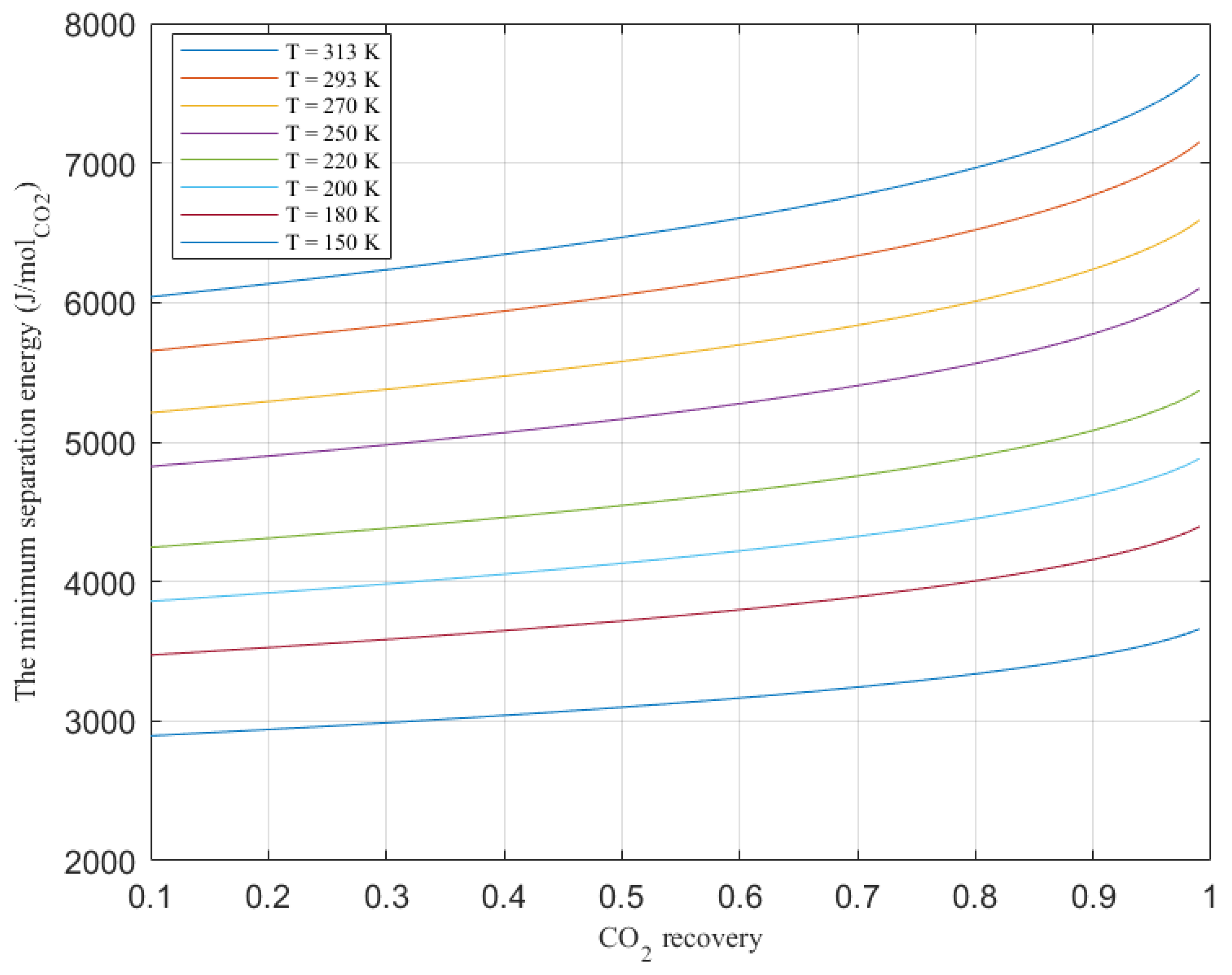
2.2.5. Minimum Energy Model

This model can be used to calculate the minimum energy required for the separation of CO₂ from the flue gases in the cryogenic process. Therefore, this model describes an ideal cryogenic carbon capture process that does not have any energy loss in the form of work or heat [59]. In this model, as Equation (62) indicates, the minimum energy required to separate a mixed gas stream into constituent pure components considering the ideal gas assumption equals to the difference in Gibbs Energy between the mixed and separated gas streams.

$$E_{min}=\mathsf{\Delta }{G}_{mix}=T\mathsf{\Delta }{S}_{mix}=-RT{{\displaystyle \sum }}_i{x}_{i}ln\left(x_i\right)$$

(62)

where $E_{min}$, $\Delta G_{mix}$, T, $\Delta S_{mix}$, and R represents the minimum energy required for separating the mixed stream gas into its pure components, the Gibbs energy of mixing, temperature, the entropy of mixing, and universal gas constant, respectively, while subscription $x_i$ denotes the mole fraction of ith species. Therefore, for the separation of CO₂ from the flue gases with a specified capture percentage, the minimum energy required for capturing CO₂ can be presented as follows:

$$\begin{array}{l}{E}_{min}=-\frac{RT}{\eta x_{C{O}_2}}(\left(x_{C{O}_2}ln{x}_{C{O}_2}+\left(1-x_{C{O}_2}\right)ln\left(1-x_{C{O}_2}\right)\right)-\left(1-\eta x_{C{O}_2}\right)\left(1-\eta \right)x_{C{O}_2}ln\left(\left(1-\eta \right)x_{C{O}_2}\right)+(1\\ \hspace{1em}\hspace{1em}\hspace{1em}\hspace{1em}\hspace{1em}\hspace{1em}\hspace{1em}-\left(1-\eta \right)x_{C{O}_2}\left)ln\left(1-\left(1-\eta \right)x_{C{O}_2}\right)\right))\end{array}$$

(63)

where $\eta$ stands for CO₂ recovery. Figure 8 indicates the minimum energy which is needed to separate CO₂ from a gas mixture for different temperatures and CO₂ recovery values when the mole fraction of CO₂ in the flue gas is 13%. As can be seen, reducing the temperature results in decreasing the minimum separation energy, while increasing the CO₂ recovery results in increasing the minimum separation energy, especially when it increases from 0.9 to 0.99. Figure 8 justifies very low energy consumption in the CCC process as it separates CO₂ at low temperatures.

The minimum amount of work required for compressing the separated CO₂ in the form of solid or liquid can also be calculated as follows:

$$W_{com,min}=-{{\displaystyle \int }}_{{\upsilon }_1}^{{\upsilon }_2}Pd\upsilon$$

(64)

where $W_{com,min}$ is the minimum compression work, while P represents pressure and $\upsilon$ denotes the volume of the compressed substance from state 1 to state 2. It is also worth noting that in the case of near-isochoric solids and liquids, the amount of compression work would be very low and with a good approximation, it is negligible as it is less than 1 kJ/kg for CO₂.

2.2.6. Soave–Redlich–Kwong (SRK) Model

SRK is one of the most popular equations of states in the hydrocarbon industry [60]. It can be used to predict a solid–vapor and liquid–vapor equilibrium with adequate accuracy. However, SRK is not a perfect method for predicting liquid compressibility. Although this model has been modified and improved for different conditions and applications since it was proposed by Soave in 1972 [61,62,63], the standard form of SRK EoS is given as follows [50]:

$$P=\frac{RT}{\left(V_m-b\right)}-\frac{a}{V_m\left(V_m+b\right)}$$

(65)

where $V_m$ denotes molar volume. Like PR EoS, when SRK EoS is used to calculate the equilibrium conditions in a mixture, mixing rules should be used to calculate a and b. Therefore, these two parameters can be calculated as follows when the van der Waals mixing rule is applied:

$$a={{\displaystyle \sum }}_i^{NC}{{\displaystyle \sum }}_j^{NC}{x}_i{x}_j\left(1-k_{ij}\right){\left(a_i{a}_j\right)}^{0.5}$$

(66)

$$b={{\displaystyle \sum }}_i^{NC}{x}_i{b}_i$$

(67)

where the value of $a_i$ and $b_i$ can be calculated for each component in the mixture as follows:

$$a_i=0.42748\frac{R^2{T}_{ci}^2}{P_{ci}} [1+m_i{(1-{(\frac{T}{T_{ci}})}^{0.5})}^2$$

(68)

$$b_i=0.08664\frac{R{T}_{ci}}{P_{ci}}$$

(69)

The parameter $m$ in Equation (68) can be calculated as a function of an acentric factor for each component as follows:

$$m_i=0.48+1.574{\omega }_i-0.17{\omega }_i{}^2$$

(70)

The binary interaction parameter used in Equation (66) is given by Shen et al. [50] for several pairs including CH₄, CO₂, N₂, and C₂H₆ which are derived from HYSIS. Once a and b are determined using Equations (66)–(70), SRK EoS can be used to calculate the fugacity coefficient for each component as follows [53]:

$$ln{\phi }_i=\frac{b_i}{b}\left(z-1\right)-\ln \left(z-B\right)-\frac{A}{B}\left(\frac{2{{\displaystyle \sum }}_j^{NC}{x}_j{\left(a_i{a}_j\right)}^{0.5}\left(1-k_{ij}\right)}{a}-\frac{b_i}{b}\right)\ln (1+\frac{B}{z})$$

(71)

where A and B can be calculated by Equations (47) and (48). Once the fugacity coefficient is calculated for each component in the mixture, Equations (49) and (50) can be used for liquid–vapor equilibrium and solid–vapor equilibrium calculations.

2.2.7. ASPEN Plus Process Simulation Software

ASPEN Plus is the leading chemical process simulator and has been widely used to build process models. It can be used to improve the existing processes or design new processes. This software has also been used to model the CCC process and predict solid–vapor and liquid–vapor equilibria using the RGibbs reactor block [8,23,64,65]. In this case, the RGibbs reactor can predict the equilibrium conditions by minimizing the Gibbs energy [65,66]. This software can also perform exergy analysis and calculate the exergy loss in the process. Moreover, the energy sensitivity and genetic algorithm available in ASPEN Plus can also be used for system optimization.

Table 1. Accuracy of RGibbs block in the ASPEN Plus simulator for the calculation of CO₂ frost point temperature [66].

The Literature for Experimental Data	Average Absolute Deviation (%) for RGibbs Tool
Pikaar [67]	0.633
Agrawal et al. [68]	0.873
Le et al. [69]	1.364
Zhang et al. [70]	0.375

compares the accuracy of RGibbs block in the ASPEN Plus simulator for the calculation of CO₂ frost point temperature with the experimental data from the different literature. As can be seen, this software predicts the equilibrium conditions accurately and can be used for modeling the CCC process.

2.3. LNG Storage Tank

As mentioned before, the CCC process can store cooling energy in the form of LNG during the off-peak hours when extra energy is available in the power plant. The stored energy can be recovered with a very fast response during the peak hours to supply more electric power and meet the residential demands. Although high-quality insulation used in the storage tank can limit the ambient heat input into the LNG tank significantly, trivial heat leak from the surrounding is always unavoidable due to the temperature gradient between LNG and the ambient [71]. It is worth noting that the value of heat leakage is dependent on the structure of the tank. For instance, smaller tanks with lower storage capacities lose more cooling energy to the environment since they have the large surface area to volume ratio [72]. The heat leakage results in minor evaporation of the liquid and causes boil-off gas (BOG) generation in the tank. Moreover, heat leakage increases the temperature of the vapor phase faster than the liquid phase since the vapor phase possesses lower heat capacity than the liquid phase [73]. This temperature difference between the two phases inside the tank brings about heat conduction at the interface and stratification phenomenon [74]. The minor heat penetration from the ambient to the LNG tank also contributes to increasing the temperature of the liquid phase which is in contact with the tank walls, making it warmer than part of the liquid located in the center of the tank. This temperature gradient between the liquid phase in the center of the tank and the liquid phase close to the tank walls causes a local convection heat transfer inside the tank. As a result of local convection heat transfer, heated liquid rises to the surface and results in increasing the surface temperature and intensifying the BOG phenomenon by elevating the evaporation rate, thermal stratification, and vapor pressure.

The generation of BOG, which is discussed above, can increase the pressure inside the storage tank, and in some cases, it may cause safety problems if the BOG is not removed from the tank for a long time and vapor pressure inside the tank passes the safety limits. It has been shown that the amount of BOG formation is highly affected by design and operating conditions of the LNG tanks [71]. Hence, the modeling and simulation of storage tanks is very important since the available experimental data are very limited [73].

2.3.1. Volume of Fluid (VOF) Method

Modeling the storage of LNG in a full-scale tank requires multiphase flow models, and because of that, the VOF method is selected and discussed here. The VOF model is the Eulerian method, of which is a very popular and powerful technique for tracking the vapor–liquid interface and can be applied to a fixed Eulerian mesh [75]. This method can be used for two or more immiscible phases to determine the intersection position between the fluids. The formulation of this method is based on the fact that two or more fluids do not interpenetrate each other. This model solves a single set of momentum equations in each control volume and estimates the value of volume fraction for each phase or fluid in the cells. The value of the volume fraction in each cell for a specific phase can be 1 or 0, or a value in the range of 0–1 when the control volume is completely occupied by the phase, it is vacant of the phase, or it is partially filled with the phase, respectively. Therefore, according to Equation (72), the summation of volume fractions of all phases in each cell should be unity.

$${{\displaystyle \sum }}_{i=1}^n{\alpha }_i=1$$

(72)

where $\alpha$ is the volume fraction, while i and n represent the ith phase and the total number of phases, respectively. The interface only appears if a control volume is partially filled with pth phase.

When this method is used to track the interface, the variation in density is just considered since the temperature varies slightly and because of that other fluid properties are considered invariable [76]. Herein, the variation in density against the temperature is estimated using the Boussinesq approximation in conservation equations for mass, momentum, and energy, given as follows:

$$\frac{\partial \rho }{\partial t}+\nabla .(\rho \overrightarrow{V})=0$$

(73)

$$\frac{\partial (\rho \overrightarrow{V})}{\partial t}+\nabla .(\rho \overrightarrow{V}\overrightarrow{V})=-\nabla p-\rho \mathsf{\beta }\overrightarrow{g}(T-T_0)+\nabla . [{\mathsf{\mu }}_{eff}(\nabla \overrightarrow{V}+\nabla \overrightarrow{V^T})]+\overrightarrow{F}$$

(74)

$$\frac{\partial \rho E}{\partial t}+\nabla .(\overrightarrow{V}\left(\rho E+p\right))=\nabla .({\mathrm{k}}_{eff}\nabla T)+S_h$$

(75)

where $\rho$, $\overrightarrow{V}$, $p$, $\overrightarrow{g}$, and k represent density, velocity vector, pressure, gravity vector, and conductivity, respectively, while T and $T_0$ denote local temperature and reference temperature, respectively. $\overrightarrow{F}$ is also body force generated by surface tension at the interface and $S_h$ also denotes the energy which causes the phase change. It should be noted that in Equation (75), the effect of the gravitational field is included in the pressure term. Furthermore, in this equation, E represents the energy and can be calculated by mass-average using the following equation [77]:

$$E={{\displaystyle \sum }}_{q=1}^n\frac{{\alpha }_q{\rho }_q{E}_q}{{\alpha }_q{\rho }_q}$$

(76)

where subscription q denotes the qth phase, while n represents the number of phases. The value of energy for each phase, i.e., $E_q$, can be calculated using the temperature and specific heat of each phase. Moreover, the average method used for calculating the energy can be also used for calculating the temperature using the following equation:

$$T={{\displaystyle \sum }}_{q=1}^n\frac{{\alpha }_q{\rho }_q{T}_q}{{\alpha }_q{\rho }_q}$$

(77)

In Equation (74), $\mathsf{\beta }$ also stands for thermal expansion coefficient and can be calculated using the following equation:

$$\mathsf{\beta }=-\frac{1}{\rho }\frac{\partial \rho }{\partial T}$$

(78)

To track the interface between two phases, the continuity equation should be solved for volume fraction of the second phase as follows:

$$\frac{\partial }{\partial t}({\alpha }_v{\rho }_v)+\nabla .({\alpha }_v{\rho }_v\overrightarrow{V})=\dot{m}$$

(79)

where $\dot{m}$ is the phase change flow rate resulting from evaporation or condensation at the interface and it gets positive and negative values for evaporation and condensation processes, respectively. Subscription v also denotes vapor phase. In this case, the phase change flow rate can be presented using the Lee phase change model, as follows [78]:

$$\dot{m}=r{\alpha }_v{\rho }_v\frac{T_{sat}-T}{T_{sat}} if T<T_{sat} \left(condensation process\right)$$

(80)

$$\dot{m}=r{\alpha }_l{\rho }_l\frac{T-T_{sat}}{T_{sat}} if T>T_{sat}\left(evaporation process\right)$$

(81)

where $T_{sat}$ is saturation temperature which changes by pressure inside the tank according to Clausius–Clapeyron equation, while r is the mass transfer intensity factor. The variation in the former parameter against the pressure can be measured for liquid methane, as follows:

$$T_{sat}=0.3709e^{-15}{P}^3-3.8013e^{-10}{P}^2+17.956e^{-15}P+93.859$$

(82)

Considering an appropriate value for r has a great impact on converging the solution by keeping the interfacial temperature close to the saturation temperature [78]. According to the previous CFD studies, 0.1 ${\mathrm{s}}^{-1}$ could be the best value for r, which may guarantee a stable solution [79,80,81]. However, there are several studies which considered different values for r. For instance, 100 ${\mathrm{s}}^{-1}$ was also considered for r by [82,83]. Once the value of the phase change flow rate is obtained using Equations (80) and (81), energy source in Equation (75) can be calculated as follows:

$$S_h=L_H\dot{m}$$

(83)

where $L_H$ denotes the latent heat of evaporation.

In this method, material properties that appear in transport equations are calculated based on the volume fraction of the component phases in each control volume. In two-phase liquid–vapor flow systems, these properties can be determined as follows if the volume fraction of the liquid phase is tracked [77]:

$$k={\alpha }_l{k}_l+\left(1-{\alpha }_l\right)k_v$$

(84)

$$\rho ={\alpha }_l{\rho }_l+\left(1-{\alpha }_l\right){\rho }_v$$

(85)

$$\mathsf{\mu }={\alpha }_l{\mathsf{\mu }}_l+\left(1-{\alpha }_l\right){\mathsf{\mu }}_v$$

(86)

$$C_P=\frac{1}{\rho } [{\alpha }_l{\rho }_l{C}_{Pl}+\left(1-{\alpha }_l\right)]{\rho }_v{C}_{Pv}$$

(87)

The finite volume method can be used to discretize the partial differential equations into a system of algebraic equations. These algebraic equations can be numerically solved to provide the solution field. ANSYS FLUENT can be used as a commercial solver software for the simulation of LNG tank using VOF method discussed above [71,84]. This commercial software utilizes the finite volume method for the discretization of partial differential equations. In this case, the SIMPLE algorithm can be used for pressure–velocity coupling, while QUICK schemes are used for solving the convective terms [84]. Moreover, time discretization can be performed using a First-Order Implicit scheme and the volume fraction equation can be solved using the Geo Reconstruct scheme. The value of ${\alpha }_l$ in Equations (84)–(87) can be set if the filling level is known.

To set the required boundary conditions for the simulation, a convective heat transfer with air which is surrounding the tank can be imposed on the exterior boundary [84]:

$$-k\frac{\partial T}{\partial n}=h\left(T-T_{ext}\right)$$

(88)

where $T_{ext}$ represents external temperature. The value considered for the heat transfer coefficient in Equation (88) is also 7 $\frac{W}{m^{2}K}$, while k also represents the thermal conductivity of evacuated perlite used as thermal insulation and can be calculated using the following equation for different temperatures in Kelvin:

$$k\left(T\right)=1.911e-4+3.476e-12T^{3.6783}$$

(89)

On the inner wall of the tank shown which represents the interface between solid and liquid subdomains, the nonslip condition (v = 0) can be imposed. On this boundary, the continuity of heat flux and temperature should also be satisfied. To reduce the computational costs, axis boundary conditions may be imposed on the symmetry axis. To set initial conditions for the fluid subdomain, initial temperature and vapor pressure can be set to 113 K and 1.13 bar, respectively, while the initial velocity for both phases should be set to 0.

The numerical solution can be obtained in a two-step process. First, a steady state problem is solved to obtain a temperature profile tank wall by setting the tank internal wall temperature to 113 K. The calculated temperature profile is then used as the initial temperature of the wall subdomain to solve the transient problem. In this case, a smaller time step is recommended since it contributes to solution stability and convergence. Therefore, the first 20 time steps can be solved in fluid and wall subdomains with Δt = 0.001 s as the time step using the temperature profile calculated in the steady-state problem for the wall subdomain. Afterward, the value of the time step can be increased to Δt = 0.01 s to reach the end time of simulation.

The results of previous simulations using the VOF model in ANSYS FLUENT commercial solver have distinctly proven the precision of the model by predicting the BOG generation rate and temperature distribution inside the tank with high accuracy [85]. In other words, it has been shown that the simulation results of the 3D model discussed above are almost the same as the experimental results, and using a 2D planar model has also an acceptable accuracy with almost 5% error [86].

2.3.2. BWRS Model

Benedict–Webb–Rubin Equation of State (BWR EoS) can be used to model and investigate the LNG tank in the CCC process. In other words, it can be used to calculate density and enthalpy, which are two critical parameters in the calculation of BOG [72]. This model is very convenient for computer programming. In this case, the equation of state is given as follows:

$$P=\rho RT+(B_{0}RT-A_0-\frac{C_0}{T^2}+\frac{D_0}{T^3}-\frac{E_0}{T^4}){\rho }^2+\left(bRT-a\right){\rho }^3+\mathsf{\alpha }\mathrm{a}{\rho }^6+\frac{C{\rho }^3}{T^2}\left(1+\mathsf{\gamma }{\rho }^2\right)exp\left(-\mathsf{\gamma }{\rho }^2\right)$$

(90)

where $\rho$, $T$, $P$ are molar density, temperature, and pressure, respectively, while $B_0$, $A_0$, $C_0$, $D_0$, R,$\mathsf{\gamma }$, b, a, and $\mathsf{\alpha }$ are coefficients that can be found in [87]. This equation has been modified by Kenneth Starling and has resulted in the following equation called the BWRS model [72]:

$$P=\rho RT+(B_{0}RT-A_0-\frac{C_0}{T^2}+\frac{D_0}{T^3}-\frac{E_0}{T^4}){\rho }^2+(bRT-a-\frac{d}{T}){\rho }^3+\mathsf{\alpha }(\mathrm{a}+\frac{d}{T}){\rho }^6+\frac{C{\rho }^3}{T^2}(1+\mathsf{\gamma }{\rho }^2)exp(-\mathsf{\gamma }{\rho }^2)$$

(91)

A comparison between Equations (90) and (91) indicates that the BWRS model possesses one more coefficient, i.e., d, and because of that, the modified model has higher accuracy than the BWR model. Equation (91) has also been revised by Nishiumi et al. [88], which resulted in the following equation of state:

$$\begin{array}{l}P=\rho RT+\left(B_{0}RT-A_0-\frac{C_0}{T^2}+\frac{D_0}{T^3}-\frac{E_0}{T^4}\right){\rho }^2+\left(bRT-a-\frac{d}{T}-\frac{e}{T^4}-\frac{f}{T^{23}}\right){\rho }^3+\mathsf{\alpha }\left(\mathrm{a}+\frac{d}{T}+\frac{e}{T^4}+\frac{f}{T^{23}}\right){\rho }^6\\ \hspace{1em}\hspace{1em}\hspace{1em}\hspace{1em}\hspace{1em}\hspace{1em}+(\frac{C}{T^2}+\frac{g}{T^8}+\frac{h}{17}){\rho }^3\left(1+\mathsf{\gamma }{\rho }^2\right)exp\left(-\mathsf{\gamma }{\rho }^2\right)\end{array}$$

(92)

Although Equation (92) is more complicated than Equation (91), previous studies have indicated that errors in predicting thermodynamic properties can be reduced from 10 to 0.35% or lower when Equation (92) is used at reduced temperatures [88].

For convenience, the following substitutions can be made to solve Equation (92) for density:

$$\begin{gathered} R_1=RT, R_2=B_{0}RT-A_0-\frac{C_0}{T^2}+\frac{D_0}{T^3}-\frac{E_0}{T^4},R_3=bRT-a-\frac{d}{T}-\frac{e}{T^4}-\frac{f}{T^{23}} \\ 93 R_4=\mathsf{\alpha }\left(\mathrm{a}+\frac{d}{T}+\frac{e}{T^4}+\frac{f}{T^{23}}\right) \\ R_5=\frac{C}{T^2}+\frac{g}{T^8}+\frac{h}{17} \end{gathered}$$

As a result, Equation (92) will be changed to the following equation:

$$P=R_1\rho +R_2{\rho }^2+R_3{\rho }^3+R_4{\rho }^6+R_5{\rho }^3\left(1+\mathsf{\gamma }{\rho }^2\right)exp\left(-\mathsf{\gamma }{\rho }^2\right)$$

(93)

Therefore, Equation (93) can be solved for density using the bisection method or the Newton–Raphson method.

Once density is calculated for LNG, enthalpy can also be obtained, as follows [88]:

$$\begin{array}{ll}H-H^0=& \left(B_{0}RT-A_0-\frac{C_0}{T^2}+\frac{D_0}{T^3}-\frac{E_0}{T^4}\right)\rho +\left(bRT-1.5a-\frac{2d}{T}-\frac{7e}{2T^4}-\frac{13f}{T^{23}}\right){\rho }^2+\mathsf{\alpha }\left(\frac{6}{5}\mathrm{a}+\frac{7d}{5T}+\frac{2e}{T^4}+\frac{29f}{5T^{23}}\right){\rho }^5\\ & \hspace{1em}\hspace{1em}+\frac{C}{\mathsf{\gamma }{T}^2} [3-(3+\frac{\mathsf{\gamma }{\rho }^2}{2}-{\mathsf{\gamma }}^2{\rho }^{4}exp\left(-\mathsf{\gamma }{\rho }^2\right)]+\frac{g}{\mathsf{\gamma }{T}^8} [9-\frac{7}{2}\mathsf{\gamma }{\rho }^2-{\mathsf{\gamma }}^2{\rho }^4)exp\left(-\mathsf{\gamma }{\rho }^2\right)]\\ & \hspace{1em}\hspace{1em}+\frac{h}{\mathsf{\gamma }{T}^{17}} [18-\left(18+8\mathsf{\gamma }{\rho }^2-{\mathsf{\gamma }}^2{\rho }^4\right)exp\left(-\mathsf{\gamma }{\rho }^2\right)]\end{array}$$

(94)

where $H^0$ is enthalpy in the ideal gas state. After the calculation of density and enthalpy using Equations (93) and (94), the value of BOG can be calculated using the following equation:

$$\mathrm{BOG}=\frac{tm}{V\rho }$$

(95)

where V, m, and t represent the volume of the tank, rate of LNG evaporation, and time span for measuring the BOG. The following equation can be used to calculate the rate of LNG evaporation:

$$m=\frac{\mathsf{\Phi }}{\mathsf{\Delta }h}$$

(96)

where $\mathsf{\Delta }h$ represents enthalpy change, while $\mathsf{\Phi }$ is the tank heat leakage.

The results of the BWRS EoS model indicate that increasing the percentage of methane in LNG intensifies the BOG generation [72]. Moreover, for different methane percentages in the LNG composition, smaller tanks have higher BOG generation since they possess a higher surface area to volume ratio. Although the method discussed here for evaluating the LNG storage tank and BOG calculation assumes a constant temperature and density for LNG and it might not be as precise as the VOF method discussed before, it is very simple and has acceptable accuracy. As result, when details such as stream function counters, fluid velocity inside the tank, and streamlines are not needed, they can be used to evaluate the LNG storage tank in the CCC process and calculate the BOG.

2.4. Compressor

The compressor is one of the most critical components in the CCC process, consuming over 80% of the required energy in the process for compressing CO₂, natural gas, and mixed refrigerant [8]. Therefore, investigation and modeling of compressors are of paramount importance. Single-shaft turbo-compressors have been modeled and optimized in reference [89] and can be used for LNG production and cryogenic applications. However, in this part, the available models for evaluating scroll compressors and linear compressors are discussed since they are more efficient than conventional compressors. These two types of compressors, especially the novel oil-free linear compressors, are widely used to compress refrigerants in cryogenic applications.

2.4.1. Compression Process Model of Scroll Compressors

In this model, variations in temperature, mass, and pressure in different chambers can be calculated as functions of an orbiting angle. Therefore, the variation in refrigerant temperature against the orbiting angle can be specified using the following equation [90]:

$$\frac{\partial T}{\partial \theta }=\frac{1}{m{C}_V} [-T{(\frac{\partial P}{\partial T})}_V [\frac{\partial V}{\partial \theta }-\frac{\upsilon }{\omega }\left({\dot{m}}_{in}-{\dot{m}}_{out}\right)]-\sum \frac{{\dot{m}}_{in}}{\omega }\left(h-h_{in}\right)+\frac{\dot{Q}}{\omega }]$$

(97)

where $m$, $C_V$, $\theta$, $\upsilon$, $\omega$, $h$, V and $\dot{Q}$ represent the mass of refrigerant, specific heat at constant volume, scroll orbiting angle, specific volume, angular speed of compressor shaft, specific enthalpy of refrigerant, volume of the control volume, and heat flow rate, respectively. In this equation, ${\dot{m}}_{in}$ denotes the mass flow rate which enters the control volume. Based on the refrigerant mass conservation, the mass balance in the compressor is provided by the following equation [90]:

$$\frac{\partial m}{\partial \theta }=\sum \frac{{\dot{m}}_{in}}{\omega }-\sum \frac{{\dot{m}}_{out}}{\omega }$$

(98)

Equations (97) and (98) are both valid for real gases [90]. In fact, the first-order differential equation given by Equation (97) has two autonomous variables, i.e., temperature and mass. This equation needs to be integrated numerically to reach a solution. In this case, expressions used to take into account the variation in pressure with the temperature at constant specific volume and enthalpies can be obtained from an equation of the state. The required expressions in this equation including the variation in pressure with respect to temperature at a constant specific volume and enthalpies can be derived from the equation of state. However, Equation (97) requires models which can predict the mass flow rates which enter/exit each chamber and the heat transfer rate. Considering Equation (97) along with Equation (98) and an equation of state, thermophysical properties can be calculated for different values of orbiting angles in whole compression chambers.

To model the compression process for the scroll compressor, the first-order differential equations given by Equations (97) and (98) should be solved in a step-by-step procedure. Therefore, the Euler method discussed by Conte et al. [91] can be used to solve equations at any desired orbiting angle ${\theta }_j$, as follows:

$$T\left({\theta }_j\right)=T({\theta }_{j-1})+{(\frac{dT}{d\theta })}_{\theta ={\theta }_{j-1}}\mathsf{\Delta }\theta$$

(99)

$$m\left({\theta }_j\right)=m({\theta }_{j-1})+{(\frac{dm}{d\theta })}_{\theta ={\theta }_{j-1}}\mathsf{\Delta }\theta$$

(100)

where $\mathsf{\Delta }\theta$ represents the step width. To solve the above-mentioned first-order equations and obtain the pressure and temperature as a function of orbiting angle, it should be noted that several differential equations should be solved at the same time since there are several compressor chambers, and each compressor chamber possesses its own differential equations.

The following equation can be used to calculate the real amount of compressional work which needs to be carried out on the refrigerant [90]:

$${\dot{W}}_{compression}=\dot{m(}{h}_{dis}-h_{suc})-{\dot{Q}}_{avg,alum}-{\dot{Q}}_{avg,steel}$$

(101)

where $h_{dis}$, $h_{suc}$, ${\dot{Q}}_{avg,alum}$, and ${\dot{Q}}_{avg,steel}$ represent the average enthalpy of discharge gas, enthalpy of suction gas at suction pressure and suction temperature, and average heat transfer rates from steel scroll and the aluminum scroll to the refrigerant, respectively. In this case, the average heat transfer rates are given as follows:

$${\dot{Q}}_{avg,alum}=rps{{\displaystyle \sum }}_{j=1}^{MAXN}{\dot{Q}}_{alum,j}\frac{\mathsf{\Delta }\theta }{\omega }$$

(102)

$${\dot{Q}}_{avg,steel}=rps{{\displaystyle \sum }}_{j=1}^{MAXN}{\dot{Q}}_{alum,j}\frac{\mathsf{\Delta }\theta }{\omega }$$

(103)

where rps and $MAXN$ are the rotation number of the orbiting scroll per second and the number of steps, respectively, while ${\dot{Q}}_{alum,j}$, ${\dot{Q}}_{alum,j}$ denote the heat transfer rate at step j which can be calculated as discussed by Chen et al. [91]. The average enthalpy of discharge gas which is needed in Equation (101) can also be calculated as follows:

$$h_{dis}=\frac{{{\displaystyle \sum }}_{j=1}^{MAXN}{\dot{m}}_{dis,j}{h}_{dis,j }\mathsf{\Delta }\theta }{{{\displaystyle \sum }}_{j=1}^{MAXN}{\dot{m}}_{dis,j}\mathsf{\Delta }\theta }$$

(104)

where $h_{dis,j }$ and ${\dot{m}}_{dis,j}$ are the enthalpy and mass flow rate (kg/radiant) of the discharged refrigerant at the orbiting angle of ${\theta }_j$, respectively.

The isentropic compression work can also be calculated as follows [92]:

$${\dot{W}}_{isentropic}=\dot{m(}{h}_{isentropic}-h_{suc})$$

(105)

where $h_{isentropic}$ represents the isentropic enthalpy of discharge refrigerant. This parameter can be calculated based on the real gas properties and considering the inlet entropy and discharge pressure [92]. The isentropic compression work and the real compression work given by Equations (101) and (105), respectively, can be used to obtain the isentropic efficiency of the compressor, as follows:

$${\eta }_{isentropic}=\frac{{\dot{W}}_{isentropic}}{{\dot{W}}_{compression}}$$

(106)

The overall compressor efficiency can also be calculated using the following equation:

$${\eta }_{compressor}=\frac{{\dot{W}}_{isentropic}}{P}$$

(107)

where P is the power input to the compressor and can be calculated as follows:

$$P=\frac{{\dot{W}}_{compression}}{{\eta }_{motor-mechanical}}$$

(108)

${\eta }_{motor-mechanical}$ used in Equation (108) represents motor-mechanical efficiency and takes into account both mechanical losses and motor losses. This parameter can be calculated by regression carried out on the performance testing results of the compressor and using the following equation:

$${\eta }_{motor-mechanical}=a_1+a_{2}ln\frac{P_{dis}}{P_{suc}}+a_3{\dot{W}}_{compression}+a_4{\dot{W}}_{compression}ln\frac{P_{dis}}{P_{suc}}$$

(109)

where $a_1$, $a_2$, $a_3$, and $a_4$ are constants in Equation (109).

2.4.2. Linear Compressor Model

The linear compressor can be successfully used in cryogenic applications. In a linear compressor, the piston moves along a linear track, and because of that, the friction and energy loss are very low. The variation in internal energy of the linear compressor is given as follows [93]:

$$\frac{dU}{dt}={\dot{Q}}_{step}+{\dot{W}}_{shaft}+{{\displaystyle \sum }}_{in}{\dot{m}}_{in}{h}_{in}-{{\displaystyle \sum }}_{out}{\dot{m}}_{out}{h}_{out}$$

(110)

where ${\dot{Q}}_{step}$, ${\dot{m}}_{in}$, ${\dot{m}}_{out}$, $h_{in}$, and $h_{out}$ denote the heat transfer between the cylinder wall and refrigerant, inlet mass flow rate, outlet mass flow rate, and specific enthalpy of the refrigerant at the compressor inlet and outlet, respectively. ${\dot{W}}_{shaft}$ also represents the shaft power and can be calculated as follows:

$${\dot{W}}_{shaft}=-P_c\frac{d{V}_c}{dt}$$

(111)

where $P_c$ and $V_c$ are the pressure in the cylinder and volume, respectively. The variation in in-cylinder temperature can be calculated using the following equation:

$$\frac{d{T}_c}{dt}=\frac{1}{m_c{C}_v} [{\dot{Q}}_{step}+{{\displaystyle \sum }}_{in}{\dot{m}}_{in}{h}_{in}-{{\displaystyle \sum }}_{out}{\dot{m}}_{out}{h}_{out}-h_c\frac{d{m}_c}{dt}-T_c{\left(\frac{\partial P_c}{\partial T}\right)}_{V_c}\left(\frac{d{V}_c}{dt}-\frac{1}{\rho }\frac{d{m}_c}{dt}\right)]$$

(112)

where $m_c$ represents the mass of refrigerant in the compressor, while $T_c$ denotes the temperature of the refrigerant in the cylinder.

The motor efficiency of linear compressors is usually assumed to be 90% for numerical studies [93], while the volumetric efficiency for linear compressors can be calculated as follows [94]:

$${\eta }_{volumetric}=\frac{{\dot{m}}_{exp}}{{\rho }_{suction}{x}_P{f}_{res}{A}_P}$$

(113)

where ${\dot{m}}_{exp}, {\rho }_{suction}, x_P$, and $A_P$ represent the experimental mass flow rate of refrigerant, the density of suction gas, displacement of the piston, and area of the piston, respectively. The overall isentropic efficiency can also be defined using the following equation [95]:

$${\eta }_{o,isentropic}=\frac{\dot{m}\left(h_{2,s}-h_{1,s}\right)}{P}$$

(114)

where $h_{2,s}$ and $h_{1,s}$ denote the enthalpy of refrigerant in discharge and suction stages, respectively, while P is the input power to the system.

2.5. Accuracy Comparison among Models of Different Component in the CCC Process

In this investigation, the available knowledge for modeling and simulating the main components in the CCC process is presented. Table A1 summarizes the explored models and methods for different components in the CCC process. The accuracy of each model is given in terms of the average absolute deviation (AAD%) in the reviewed references. This parameter can be obtained for the desired variable when the calculated and experimental value at the ith point is represented by $variabl{e}_{cal,i}$ and $variabl{e}_{exp,i}$. Although all presented models are accurate, they possess different AAD values due to the assumptions made in the models and the utilized method for modeling. This parameter is provided by some references and calculated for others in the present investigation.

As Appendix A indicates, the differential method is mostly used to design and model the heat exchangers in the CCC process. According to this table, ASPEN Plus is a very popular commercial software to model the CCC process integrated with power plants or other industrial processes due to its exceptional capability to model thermal and chemical processes. The RGibbs reactor available in Aspen Plus can be used to accurately calculate equilibrium conditions as well as the dew point and frost point temperatures of CO₂, solid CO₂ solubility in hydrocarbon mixture, etc. Furthermore, ANSYS FLUENT as a CFD tool has also been widely used by researchers to model and evaluate the LNG storage tank. They used the VOF method in 2D and 3D dynamic models to evaluate the BOG phenomenon with acceptable accuracy. Furthermore, it was shown that the flash model based on the Rachford–Rice equation can be used to predict the SVE conditions with acceptable accuracy, especially at low pressures. This model was also extended to predict LVE conditions and calculate the dew point of CO₂. It was shown that in both cases, this simple model can be applied to predict the equilibrium conditions at low pressures without involving the complexity of mixing rules.

3. Conclusions

Although the CCC process is a new technology for CO₂ emission mitigation, different aspects of this process have been modeled and simulated using numerical methods, but several fields need to be investigated more, as follows:

• A numerical model which can predict the pressure drop in the process accurately may contribute to reaching an optimum size for tubes and heat exchangers to reduce the pressure drop without the generation of a maldistribution phenomenon.
• A dynamic model of the power plant and the CCC process, even in the case of using the integral method for modeling the heat exchangers, would provide helpful information about the transient behavior of the process.
• Modelling the desublimation heat exchanger system by using the computational fluid dynamics method can provide very helpful information about the solid–vapor equilibrium of CO₂ mixtures.

References

1. Chauhan, K. Distributed Energy Resources in Microgrids: Integration, Challenges and Optimization; Chauhan, R.K., Ed.; Academic Press: Cambridge, MA, USA, 2019. [Google Scholar]
2. Moodley, P. Sustainable biofuels: Opportunities and challenges. Sustain. Biofuels 2021, 1–20. [Google Scholar] [CrossRef]
3. Liu, Z.; Deng, Z.; Davis, S.J.; Giron, C.; Ciais, P. Monitoring global carbon emissions in 2021. Nat. Rev. Earth Environ. 2022, 3, 217–219. [Google Scholar] [CrossRef] [PubMed]
4. He, J.; Deng, J.; Su, M. CO2 emission from China’s energy sector and strategy for its control. Energy 2010, 35, 4494–4498. [Google Scholar] [CrossRef]
5. Jansen, D.; Gazzani, M.; Manzolini, G.; Van Dijk, E.; Carbo, M. Pre-combustion CO2 capture. Int. J. Greenh. Gas Control 2015, 40, 167–187. [Google Scholar] [CrossRef]
6. Stanger, R.; Wall, T.; Spörl, R.; Paneru, M.; Grathwohl, S.; Weidmann, M.; Scheffknecht, G.; McDonald, D.; Myöhänen, K.; Ritvanen, J.; et al. Oxyfuel combustion for CO2 capture in power plants. Int. J. Greenh. Gas Control 2015, 40, 55–125. [Google Scholar] [CrossRef]
7. Zheng, C.; Liu, Z.; Xiang, J.; Zhang, L.; Zhang, S.; Luo, C.; Zhao, Y. Fundamental and Technical Challenges for a Compatible Design Scheme of Oxyfuel Combustion Technology. Engineering 2015, 1, 139–149. [Google Scholar] [CrossRef]
8. Jensen, M. Energy Process Enabled by Cryogenic Carbon Capture. Ph.D. Thesis, Brigham Young University, Provo, UT, USA, 2015. [Google Scholar]
9. Skorek-Osikowska, A.; Janusz-Szymańska, K.; Kotowicz, J. Modeling and analysis of selected carbon dioxide capture methods in IGCC systems. Energy 2012, 45, 92–100. [Google Scholar] [CrossRef]
10. Sanchez Fernandez, E.; Goetheer, E.L.V.; Manzolini, G.; Macchi, E.; Rezvani, S.; Vlugt, T.J.H. Thermodynamic assessment of amine based CO2 capture technologies in power plants based on European Benchmarking Task Force methodology. Fuel 2014, 129, 318–329. [Google Scholar] [CrossRef]
11. Zaman, M.; Lee, J.H. Carbon capture from stationary power generation sources: A review of the current status of the technologies. Korean J. Chem. Eng. 2013, 30, 1497–1526. [Google Scholar] [CrossRef]
12. Duan, L.; Zhao, M.; Yang, Y. Integration and optimization study on the coal-fired power plant with CO2 capture using MEA. Energy 2012, 45, 107–116. [Google Scholar] [CrossRef]
13. Amrollahi, Z.; Ystad, P.A.M.; Ertesvåg, I.S.; Bolland, O. Optimized process configurations of post-combustion CO2 capture for natural-gas-fired power plant—Power plant efficiency analysis. Int. J. Greenh. Gas Control 2012, 8, 1–11. [Google Scholar] [CrossRef]
14. Scholes, C.A.; Ho, M.T.; Aguiar, A.A.; Wiley, D.E.; Stevens, G.W.; Kentish, S.E. Membrane gas separation processes for CO2 capture from cement kiln flue gas. Int. J. Greenh. Gas Control 2014, 24, 78–86. [Google Scholar] [CrossRef]
15. Font-Palma, C.; Cann, D.; Udemu, C. Review of Cryogenic Carbon Capture Innovations and Their Potential Applications. C 2021, 7, 58. [Google Scholar] [CrossRef]
16. Safdarnejad, S.M.; Hedengren, J.D.; Baxter, L.L. Dynamic optimization of a hybrid system of energy-storing cryogenic carbon capture and a baseline power generation unit. Appl. Energy 2016, 172, 66–79. [Google Scholar] [CrossRef]
17. Song, C.; Kitamura, Y.; Li, S. Energy analysis of the cryogenic CO2 capture process based on Stirling coolers. Energy 2014, 65, 580–589. [Google Scholar] [CrossRef]
18. Baxter, L.; Baxter, A.; Burt, S. Cryogenic CO2 Capture as a Cost-Effective CO2 Capture Process. In Proceedings of the 26th Annual International Pittsburgh Coal Conference 2009, PCC 2009, Pittsburgh, PA, USA, 20–23 September 2009; Volume 1. [Google Scholar]
19. Song, C.; Liu, Q.; Deng, S.; Li, H.; Kitamura, Y. Cryogenic-based CO2 capture technologies: State-of-the-art developments and current challenges. Renew. Sustain. Energy Rev. 2019, 101, 265–278. [Google Scholar] [CrossRef]
20. Zhang, J.; Meerman, H.; Benders, R.; Faaij, A. Comprehensive review of current natural gas liquefaction processes on technical and economic performance. Appl. Therm. Eng. 2020, 166, 114736. [Google Scholar] [CrossRef]
21. Berstad, D.; Anantharaman, R.; Nekså, P. Low-temperature CO2 capture technologies—Applications and potential. Int. J. Refrig. 2013, 36, 1403–1416. [Google Scholar] [CrossRef]
22. Willson, P.; Lychnos, G.; Clements, A.; Michailos, S.; Font-Palma, C.; Diego, M.E.; Pourkashanian, M.; Howe, J. Evaluation of the performance and economic viability of a novel low temperature carbon capture process. Int. J. Greenh. Gas Control 2019, 86, 1–9. [Google Scholar] [CrossRef]
23. Fazlollahi, F.; Bown, A.; Ebrahimzadeh, E.; Baxter, L.L. Design and analysis of the natural gas liquefaction optimization process- CCC-ES (energy storage of cryogenic carbon capture). Energy 2015, 90, 244–257. [Google Scholar] [CrossRef] [Green Version]
24. Yuan, Z.; Cui, M.; Xie, Y.; Li, C. Design and analysis of a small-scale natural gas liquefaction process adopting single nitrogen expansion with carbon dioxide pre-cooling. Appl. Therm. Eng. 2014, 64, 139–146. [Google Scholar] [CrossRef]
25. Van Nguyen, T.; Rothuizen, E.D.; Markussen, W.B.; Elmegaard, B. Thermodynamic comparison of three small-scale gas liquefaction systems. Appl. Therm. Eng. 2018, 128, 712–724. [Google Scholar] [CrossRef]
26. Remeljej, C.W.; Hoadley, A.F.A. An exergy analysis of small-scale liquefied natural gas (LNG) liquefaction processes. Energy 2006, 31, 2005–2019. [Google Scholar] [CrossRef]
27. Qyyum, M.A.; He, T.; Qadeer, K.; Mao, N.; Lee, S.; Lee, M. Dual-effect single-mixed refrigeration cycle: An innovative alternative process for energy-efficient and cost-effective natural gas liquefaction. Appl. Energy 2020, 268, 115022. [Google Scholar] [CrossRef]
28. Kamath, R.S.; Grossmann, I.E.; Biegler, L.T. Modeling of Multi-Stream Heat Exchangers with Phase Changes for Cryogenic Applications. Comput. Aided Chem. Eng. 2009, 27, 921–926. [Google Scholar]
29. Haider, P.; Freko, P.; Acher, T.; Rehfeldt, S.; Klein, H. A transient three-dimensional model for thermo-fluid simulation of cryogenic plate-fin heat exchangers. Appl. Therm. Eng. 2020, 180, 115791. [Google Scholar] [CrossRef]
30. Martynov, S.; Brown, S.; Mahgerefteh, H. An extended Peng-Robinson equation of state for carbon dioxide solid-vapor equilibrium. Greenh. Gases 2013, 3, 136–147. [Google Scholar] [CrossRef]
31. Wibawa, G.; Nafi, M.F.; Permatasari, A.; Mustain, A. Application of Peng-Robinson Equation of State for Calculating Solid-Vapor and Solid-Liquid Equilibrium of CH4-CO2 System. Mod. Appl. Sci. 2015, 9, 177. [Google Scholar] [CrossRef]
32. Ali, A.; Abdulrahman, A.; Garg, S.; Maqsood, K.; Murshid, G. Application of artificial neural networks (ANN) for vapor-liquid-solid equilibrium prediction for CH4-CO2 binary mixture. Greenh. Gases 2018, 9, 67–78. [Google Scholar] [CrossRef]
33. Reddy, H.V.; Bisen, V.S.; Rao, H.N.; Dutta, A.; Garud, S.S.; Karimi, I.A.; Farooq, S. Towards energy-efficient LNG terminals: Modeling and simulation of reciprocating compressors. Comput. Chem. Eng. 2019, 128, 312–321. [Google Scholar] [CrossRef]
34. Fang, X.; Chen, W.; Zhou, Z.; Xu, Y. Empirical models for efficiency and mass flow rate of centrifugal compressors. Int. J. Refrig. 2014, 41, 190–199. [Google Scholar] [CrossRef]
35. Wang, M.; Zhang, J.; Xu, Q.; Li, K. Thermodynamic-analysis-based energy consumption minimization for natural gas liquefaction. Ind. Eng. Chem. Res. 2011, 50, 12630–12640. [Google Scholar] [CrossRef]
36. Prasad, B.S.V.; Gurukul, S.M.K.A. Differential Methods for the Performance Prediction of Multistream Plate-Fin Heat Exchangers. J. Heat Transf. 1992, 114, 41–49. [Google Scholar] [CrossRef]
37. You, Y.; Fan, A.; Huang, S.; Liu, W. Numerical modeling and experimental validation of heat transfer and flow resistance on the shell side of a shell-and-tube heat exchanger with flower baffles. Int. J. Heat Mass Transf. 2012, 55, 7561–7569. [Google Scholar] [CrossRef]
38. He, Y.; Tao, W.; Deng, B.; Li, X.; Wu, Y. Numerical simulation and experimental study of flow and heat transfer characteristics of shell side fluid in shell-and-tube heat exchangers. In Proceedings of the Engineering Conferences International, Hoboken, NJ, USA, September 2005; pp. 29–42. [Google Scholar]
39. Haider, P.; Heinz, P.; Acher, T.; Rehfeldt, S.; Klein, H. A Framework for Multi-Objective Optimization of Plate-Fin Heat Exchangers Using a Detailed Three-Dimensional Simulation Model. ChemEngineering 2021, 5, 82. [Google Scholar] [CrossRef]
40. Taler, D. Modelowanie matematyczne pracy wymiennika ciepła z rur ożebrowanych dla zmiennych w czasie strumienia masy płynu i prędkości powietrza. Czas. Tech. 2017, 3, 183–196. [Google Scholar] [CrossRef]
41. Wang, Z.; Sundén, B.; Li, Y. A novel optimization framework for designing multi-stream compact heat exchangers and associated network. Appl. Therm. Eng. 2017, 116, 110–125. [Google Scholar] [CrossRef]
42. Prasad, B.S.V.; Gurukul, S.M.K.A. Differential method for sizing multistream plate fin heat exchangers. Cryogenics 1987, 27, 257–262. [Google Scholar] [CrossRef]
43. De Guido, G.; Pellegrini, L.A. Calculation of solid-vapor equilibria for cryogenic carbon capture. Comput. Chem. Eng. 2022, 156, 107569. [Google Scholar] [CrossRef]
44. William James, D.; William, D. Failing Drop CO2 Deposition (Desublimation) Heat Exchanger for Failing Drop CO2 Deposition (Desublimation) Heat Exchanger for the Cryogenic Carbon Capture Process. Master’s Thesis, Brigham Young University, Provo, UT, USA, 2011. [Google Scholar]
45. Bloxham, J.C.; Redd, M.E.; Giles, N.F.; Knotts, T.A.; Wilding, W.V. Proper Use of the DIPPR 801 Database for Creation of Models, Methods, and Processes. J. Chem. Eng. Data 2021, 66, 3–10. [Google Scholar] [CrossRef]
46. Tuinier, M.J.; Hamers, H.P.; Van Sint Annaland, M. Techno-economic evaluation of cryogenic CO2 capture-A comparison with absorption and membrane technology. Int. J. Greenh. Gas Control 2011, 5, 1559–1565. [Google Scholar] [CrossRef]
47. Tuinier, M.J.; van Sint Annaland, M.; Kuipers, J.A.M. A novel process for cryogenic CO2 capture using dynamically operated packed beds—An experimental and numerical study. Int. J. Greenh. Gas Control 2011, 5, 694–701. [Google Scholar] [CrossRef]
48. Schiesser, W.E.; Griffiths, G.W. A Compendium of Partial Differential Equation Models: Method of Lines Analysis with Matlab; Cambridge University Press: Cambridge, UK, 2009. [Google Scholar]
49. Smit, J.; Van Sint Annaland, M.; Kuipers, J.A.M. Grid adaptation with WENO schemes for non-uniform grids to solve convection-dominated partial differential equations. Chem. Eng. Sci. 2005, 60, 2609–2619. [Google Scholar] [CrossRef]
50. Shen, T.; Gao, T.; Lin, W.; Gu, A. Determination of CO2 Solubility in Saturated Liquid CH4 + N2 and CH4 + C2H6 Mixtures above Atmospheric Pressure. J. Chem. Eng. Data 2012, 57, 2296–2303. [Google Scholar] [CrossRef]
51. Lopez-Echeverry, J.S.; Reif-Acherman, S.; Araujo-Lopez, E. Peng-Robinson equation of state: 40 years through cubics. Fluid Phase Equilib. 2017, 447, 39–71. [Google Scholar] [CrossRef]
52. Stryjek, R.; Vera, J.H. PRSV: An improved peng—Robinson equation of state for pure compounds and mixtures. Can. J. Chem. Eng. 1986, 64, 323–333. [Google Scholar] [CrossRef]
53. Yang, W.; Li, S.; Li, X.; Liang, Y.; Zhang, X. Analysis of a new liquefaction combined with desublimation system for CO2 separation based on N2/CO2 phase equilibrium. Energies 2015, 8, 9495–9508. [Google Scholar] [CrossRef]
54. ZareNezhad†, B. Prediction of CO2 freezing points for the mixtures of CO2-CH4 at cryogenic conditions of NGL extraction plants. Korean J. Chem. Eng 2006, 23, 827–831. [Google Scholar] [CrossRef]
55. Aspen Plus® Burlington; Version 9; Aspen Technology, Inc.: Bedford, MA, USA, 2016.
56. Abu-Eishah, S.I. Calculation of vapour-liquid equilibrium data for binary chlorofluorocarbon mixtures using the Peng-Robinson equation of state. Fluid Phase Equilib. 1991, 62, 41–52. [Google Scholar] [CrossRef]
57. Jensen, M.J.; Russell, C.S.; Bergeson, D.; Hoeger, C.D.; Frankman, D.J.; Bence, C.S.; Baxter, L.L. Prediction and validation of external cooling loop cryogenic carbon capture (CCC-ECL) for full-scale coal-fired power plant retrofit. Int. J. Greenh. Gas Control 2015, 42, 200–212. [Google Scholar] [CrossRef]
58. Baxter, L.; Hoeger, C.; Stitt, K.; Burt, S.; Baxter, A. Cryogenic Carbon CaptureTM (CCC) Status Report. In Proceedings of the 15th Greenhouse Gas Control Technologies Conference, Abu Dhabi, UAE, 15–18 March 2021. [Google Scholar] [CrossRef]
59. Berger, A.H.; Hoeger, C.; Baxter, L.; Bhown, A. Evaluation of Cryogenic Systems for Post Combustion CO2 Capture. In Proceedings of the 14th International Conference on Greenhouse Gas Control Technologies, GHGT-14, Melbourne, Australia, 21–25 October 2018; Volume 1, pp. 1–8. [Google Scholar] [CrossRef]
60. Li, H.; Yan, J. Impacts of equations of state (EOS) and impurities on the volume calculation of CO2 mixtures in the applications of CO2 capture and storage (CCS) processes. Appl. Energy 2009, 86, 2760–2770. [Google Scholar] [CrossRef]
61. Kabadi, V.N.; Danner, R.P. A Modified Soave-Redlich-Kwong Equation of State for Water-Hydrocarbon Phase Equilibria. Ind. Eng. Chem. Process Des. Dev. 1985, 24, 537–541. [Google Scholar] [CrossRef]
62. Wang, P.; Huang, S.; Zhao, F.; Shi, J.; Wang, B.; Li, Y. Modeling phase behavior of nano-confined fluids in shale reservoirs with a modified Soave-Redlich-Kwong equation of state. Chem. Eng. J. 2022, 433, 133661. [Google Scholar] [CrossRef]
63. Valderrama, J.O.; Silva, A. Modified Soave-Redlich-Kwong equations of state applied to mixtures containing supercritical carbon dioxide. Korean J. Chem. Eng. 2003, 20, 709–715. [Google Scholar] [CrossRef]
64. Sateesh, C.; Nandakishora, Y.; Sahoo, R.K.; Murugan, S. Study of cryogenic CO2 capture with solar-assisted VAR system. Clean. Eng. Technol. 2021, 5, 100351. [Google Scholar] [CrossRef]
65. Pellegrini, L.A.; De Guido, G.; Ingrosso, S. Thermodynamic Framework for Cryogenic Carbon Capture. Comput. Aided Chem. Eng. 2020, 48, 475–480. [Google Scholar]
66. De Guido, G.; Pellegrini, L.A. Phase Equilibria Analysis in the Presence of Solid Carbon Dioxide. Chem. Eng. Trans. 2021, 86, 1261–1266. [Google Scholar]
67. Pikaar, M.J. A Study of Phase Equilibria in Hydrocarbon-CO2 Systems. Ph.D. Thesis, University of London, London, UK, 1959. [Google Scholar]
68. Agrawal, G.M.; Laverman, R.J. Phase behavior of the methane-carbon dioxide system in the solid-vapor region. In Advances in Cryogenic Engineering; Springer: Boston, MA, USA, 1995; pp. 327–338. [Google Scholar]
69. Le, T.T.; Trebble, M.A. Measurement of carbon dioxide freezing in mixtures of methane, ethane, and nitrogen in the solid-vapor equilibrium region. J. Chem. Eng. Data 2007, 52, 683–686. [Google Scholar] [CrossRef]
70. Zhang, L.; Burgass, R.; Chapoy, A.; Tohidi, B.; Solbraa, E. Measurement and modeling of CO2 frost points in the CO2-methane systems. J. Chem. Eng. Data 2011, 56, 2971–2975. [Google Scholar] [CrossRef]
71. Saleem, A. CFD Study of Large-Scale LNG Storage and Carbon Capture Systems. Ph.D. Thesis, National University of Singapore, Singapore, 2020. [Google Scholar]
72. Adom, E.; Islam, S.Z.; Ji, X. Modelling of Boil-off Gas in LNG tanks: A case study. Int. J. Eng. Technol. 2010, 2, 292–296. [Google Scholar]
73. Al Ghafri, S.Z.S.; Perez, F.; Heum Park, K.; Gallagher, L.; Warr, L.; Stroda, A.; Siahvashi, A.; Ryu, Y.; Kim, S.; Kim, S.G.; et al. Advanced boil-off gas studies for liquefied natural gas. Appl. Therm. Eng. 2021, 189, 116735. [Google Scholar] [CrossRef]
74. Kang, M.; Kim, J.; You, H.; Chang, D. Experimental investigation of thermal stratification in cryogenic tanks. Exp. Therm. Fluid Sci. 2018, 96, 371–382. [Google Scholar] [CrossRef]
75. Jabbari, M.; Bulatova, R.; Hattel, J.H.; Bahl, C.R.H. An evaluation of interface capturing methods in a VOF based model for multiphase flow of a non-Newtonian ceramic in tape casting. Appl. Math. Model. 2014, 38, 3222–3232. [Google Scholar] [CrossRef]
76. Sundén, B.; Fu, J. Heat Transfer in Aerospace Applications; Academic Press: Cambridge, MA, USA, 2016. [Google Scholar]
77. Saleem, A.; Farooq, S.; Karimi, I.A.; Banerjee, R. A CFD simulation study of boiling mechanism and BOG generation in a full-scale LNG storage tank. Comput. Chem. Eng. 2018, 115, 112–120. [Google Scholar] [CrossRef]
78. Sun, D.; Xu, J.; Chen, Q. Modeling of the evaporation and condensation phase-change problems with FLUENT. Numer. Heat Transf. Part B Fundam. 2014, 66, 326–342. [Google Scholar] [CrossRef]
79. Wu, H.L.; Peng, X.F.; Ye, P.; Eric Gong, Y. Simulation of refrigerant flow boiling in serpentine tubes. Int. J. Heat Mass Transf. 2007, 50, 1186–1195. [Google Scholar] [CrossRef]
80. De Schepper, S.C.K.; Heynderickx, G.J.; Marin, G.B. Modeling the evaporation of a hydrocarbon feedstock in the convection section of a steam cracker. Comput. Chem. Eng. 2009, 33, 122–132. [Google Scholar] [CrossRef]
81. Alizadehdakhel, A.; Rahimi, M.; Alsairafi, A.A. CFD modeling of flow and heat transfer in a thermosyphon. Int. Commun. Heat Mass Transf. 2010, 37, 312–318. [Google Scholar] [CrossRef]
82. Yang, Z.; Peng, X.F.; Ye, P. Numerical and experimental investigation of two phase flow during boiling in a coiled tube. Int. J. Heat Mass Transf. 2008, 51, 1003–1016. [Google Scholar] [CrossRef]
83. Goodson, K.; Rogacs, A.; David, M.; Fang, C. Volume of fluid simulation of boiling two-phase flow in a vapor-venting microchannel. Front. Heat Mass Transf. 2010, 1, 013002. [Google Scholar]
84. Ferrín, J.L.; Pérez-Pérez, L.J. Numerical simulation of natural convection and boil-off in a small size pressurized LNG storage tank. Comput. Chem. Eng. 2020, 138, 106840. [Google Scholar] [CrossRef]
85. Wu, S.; Ju, Y.; Lin, J.; Fu, Y. Numerical simulation and experiment verification of the static boil-off rate and temperature field for a new independent type B liquefied natural gas ship mock up tank. Appl. Therm. Eng. 2020, 173, 115265. [Google Scholar] [CrossRef]
86. Wu, S.; Ju, Y. Numerical study of the boil-off gas (BOG) generation characteristics in a type C independent liquefied natural gas (LNG) tank under sloshing excitation. Energy 2021, 223, 120001. [Google Scholar] [CrossRef]
87. Reid, R.C.; Prausnitz, J.M.; Poling, B.E. The Properties of Gases and Liquids; McGraw Hill: New York, NY, USA, 1987. [Google Scholar]
88. Nishiumi, H.; Saito, S. An improved generalized BWR equation of state applicable to low reduced temperatures. J. Chem. Eng. Japan 1975, 8, 356–360. [Google Scholar] [CrossRef]
89. Faruque Hasan, M.M.; Razib, M.S.; Karimi, I.A. Optimization of Compressor Networks in LNG Operations; Elsevier Inc.: Amsterdam, The Netherlands, 2009; Volume 27. [Google Scholar]
90. Chen, Y.; Halm, N.P.; Groll, E.A.; Braun, J.E. Mathematical modeling of scroll compressors—Part I: Compression process modeling. Int. J. Refrig. 2002, 25, 731–750. [Google Scholar] [CrossRef]
91. Conte, S.D.; De Boor, C. Elementary Numerical Analysis: An Algorithmic Approach; Society for Industrial and Applied Mathematics: Philadelphia, PA, USA, 2017. [Google Scholar]
92. Chen, Y.; Halm, N.P.; Braun, J.E.; Groll, E.A. Mathematical modeling of scroll compressors—Part II: Overall scroll compressor modeling. Int. J. Refrig. 2002, 25, 751–764. [Google Scholar] [CrossRef]
93. Shen, H.; Li, Z.; Liang, K.; Chen, X. Numerical modeling of a novel two-stage linear refrigeration compressor. Int. J. Low-Carbon Technol. 2022, 17, 436–445. [Google Scholar] [CrossRef]
94. Bradshaw, C.R.; Groll, E.A.; Garimella, S.V. A comprehensive model of a miniature-scale linear compressor for electronics cooling. Int. J. Refrig. 2011, 34, 63–73. [Google Scholar] [CrossRef]
95. Bijanzad, A.; Hassan, A.; Lazoglu, I.; Kerpicci, H. Development of a new moving magnet linear compressor. Part B: Performance analysis. Int. J. Refrig. 2020, 113, 94-002. [Google Scholar] [CrossRef]
96. Schach, M.O.; Oyarzún, B.; Schramm, H.; Schneider, R.; Repke, J.U. Feasibility study of CO2 capture by anti-sublimation. Energy Procedia 2011, 4, 1403–1410. [Google Scholar] [CrossRef]
97. Lee, H.; Jung, I.; Roh, G.; Na, Y.; Kang, H. Comparative analysis of on-board methane and methanol reforming systems combined with HT-PEM fuel cell and CO2 capture/liquefaction system for hydrogen fueled ship application. Energies 2020, 13, 224. [Google Scholar] [CrossRef]
98. Shirmohammadi, R.; Aslani, A.; Ghasempour, R.; Romeo, L.M.; Petrakopoulou, F. Process design and thermoeconomic evaluation of a CO2 liquefaction process driven by waste exhaust heat recovery for an industrial CO2 capture and utilization plant. J. Therm. Anal. Calorim. 2021, 145, 1585–1597. [Google Scholar] [CrossRef]
99. Fazlollahi, F.; Bown, A.; Ebrahimzadeh, E.; Baxter, L.L. Transient natural gas liquefaction and its application to CCC-ES (energy storage with cryogenic carbon captureTM). Energy 2016, 103, 369–384. [Google Scholar] [CrossRef] [Green Version]
100. Zhang, X.; Singh, B.; He, X.; Gundersen, T.; Deng, L.; Zhang, S. Post-combustion carbon capture technologies: Energetic analysis and life cycle assessment. Int. J. Greenh. Gas Control 2014, 27, 289–298. [Google Scholar] [CrossRef] [Green Version]
Figure 1. Flue gas pre-processing before entering CCC process.
Energies 16 01855 g001
Figure 2. A simplified schematic of the CCC process based on reference [8,23].
Energies 16 01855 g002
Figure 3. The models for each component and their applications in the CCC process.
Energies 16 01855 g003
Figure 4. Discretization of a counter-flow heat exchanger into N sections for temperature calculation using the differential method.
Energies 16 01855 g004
Figure 5. Comparison of calculated SVE temperature using the Rachford–Rice model against the proposed approach in [18].
Energies 16 01855 g005
Figure 6. SVE temperature for different CO2 recovery values for different flue gas pressures.
Energies 16 01855 g006
Figure 7. Comparing the calculated LVE temperature using the Rachford–Rice model with the literature [53].
Energies 16 01855 g007
Figure 8. Minimum energy for separation of CO2 from a gas mixture for different temperatures and CO2 recovery values when the CO2 mole fraction is 13%.
Energies 16 01855 g008