
An Integrated Approach to Reservoir Characterization for Evaluating Shale Productivity of Duvernary Shale: Insights from Multiple Linear Regression

Abstract
:1. Introduction
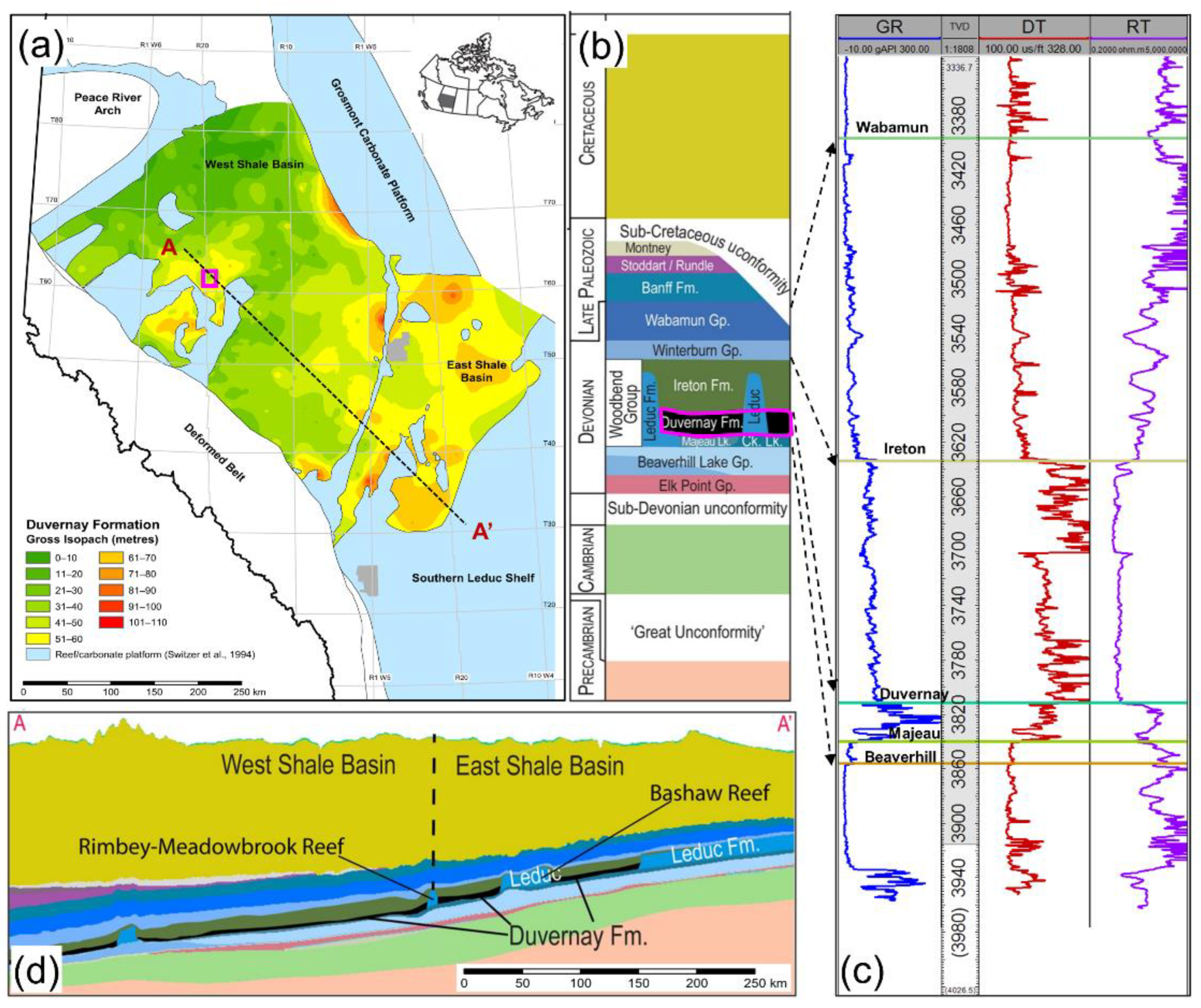
2. Field Background
3. Methodology
3.1. Experimentally Based Reservoir Parameters
3.2. Multiple LINEAR Regression Approach
4. Results
4.1. Characterization of Reservoir Properties
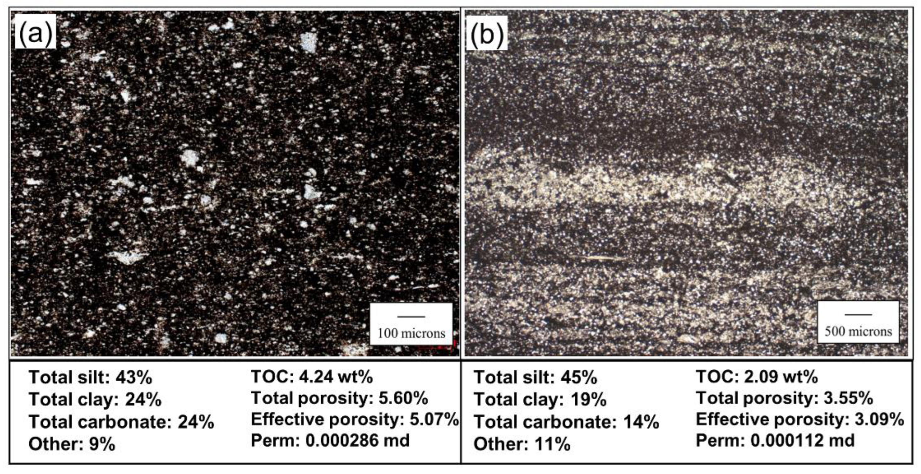
4.1.1. Mineralogy Characterization
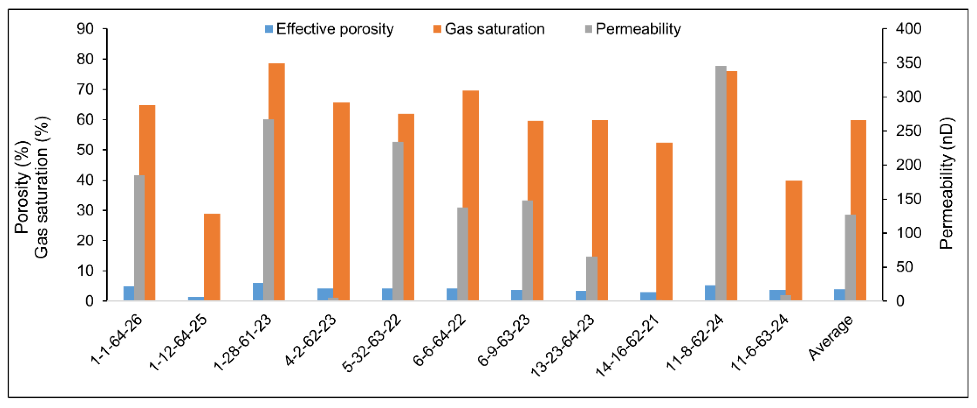
4.1.2. Petrophysics Characterization
4.1.3. Geochemistry Characterization
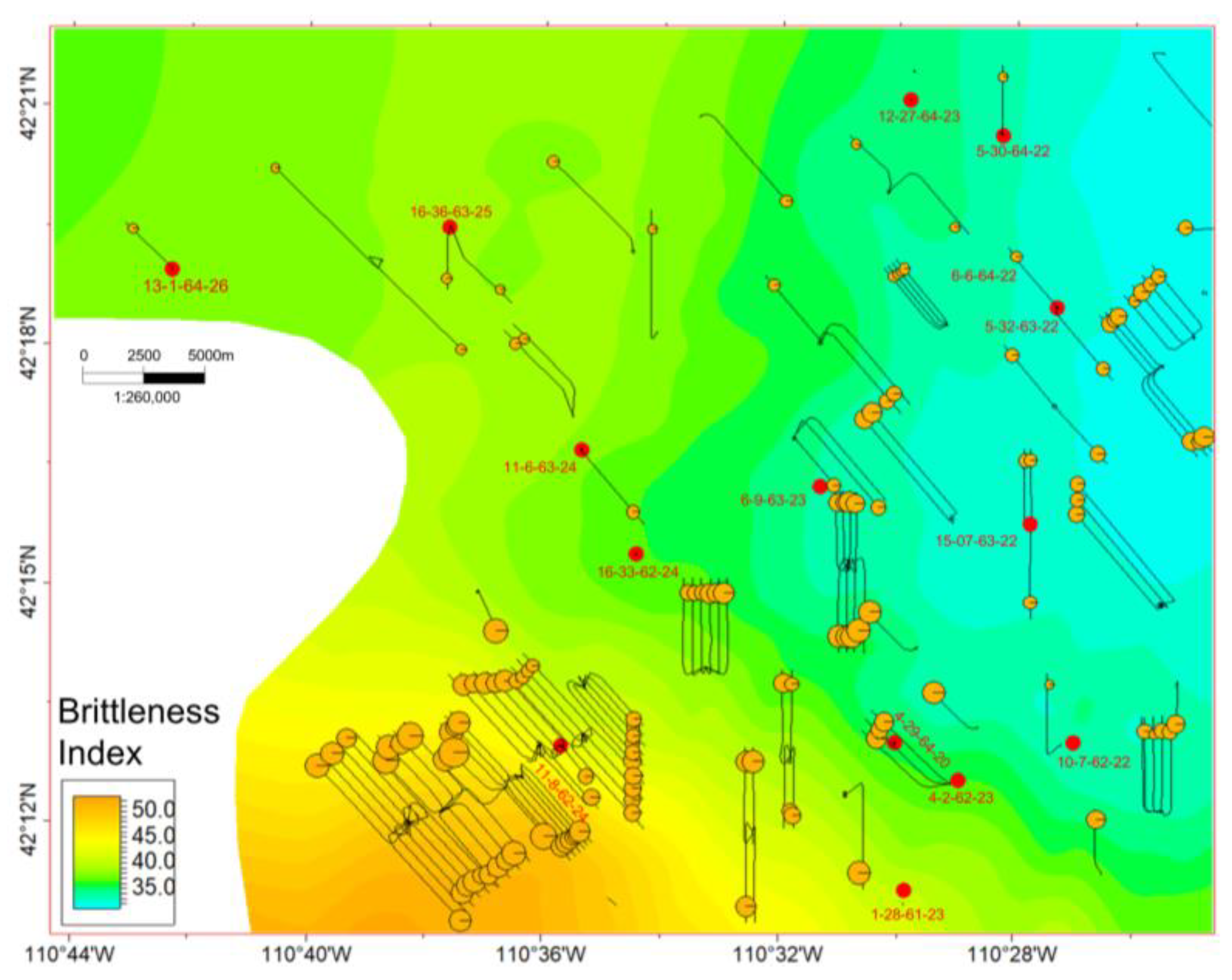
4.1.4. Geomechanics Characterization
4.2. MLR-Based Prediction Model
5. Discussions
5.1. Data Quality
5.2. Reservoir Properties
5.3. Data-Mining Methods
5.4. Regional-Level Assessment
6. Conclusions
Author Contributions
Funding
Data Availability Statement
Acknowledgments
Conflicts of Interest
Nomenclature
| BI | brittleness index |
| BMC | brittle mineral content |
| ESB | Eastern Shale Basin |
| FESEM | field emission scanning electron microscope |
| HI | hydrogen index |
| MLR | multiple linear regression |
| OI | oxygen index |
| PI | production index |
| S1 | adsorbed hydrocarbons |
| S2 | kerogen pyrolysis |
| Sg | gas saturation |
| SGS | sequential Gaussian stochastic |
| Tmax | maximum pyrolysis yield temperature |
| TOC | total organic carbon |
| Vcl | clay content |
| VR | vitrinite reflectance |
| WCSB | Western Canadian Sedimentary Basin |
| WSB | Western Shale Basin |
| Φ | effective porosity |
| ai | an original independent variable at one site |
| amax | maximum value among all “a” values |
| amin | minimum value among all “a” values |
| n | number of parameters |
| xi | ith standardized independent variable |
| Y | dependent variable |
| yj | jth parameter after normalization |
| mean value of predicted parameters | |
| predicted jth parameter | |
| β0 | y-intercept |
| βi | regression coefficient of the ith independent variables |
| ε | model error |
References
- Li, Q.; Chen, M.; Fred, P.W.; Jin, Y.; Li, Z. Influences of engineering factors on shale gas productivity: A case study from the Haynesville shale gas reservoir in North America. Nat. Gas Ind. 2012, 32, 54–59. [Google Scholar]
- Wan, Y.; Li, Z.; Lu, B. The development of Fayetteville shale play and its implications. Nat. Gas Geosci. 2019, 30, 1655–1666. [Google Scholar]
- Zou, C.; Pan, S.; Jing, Z.; Gao, J.; Yang, Z.; Wu, S.; Zhao, Q. Shale oil and gas revolution and its impact. Acta Pet. Sin. 2020, 41, 1–12. [Google Scholar]
- IEA. Natural Gas Information: Overview; IEA: Paris, France, 2021; Available online: https://www.iea.org/reports/natural-gas-information-overview (accessed on 1 November 2022).
- Zhao, W.; Xia, M.; Zhang, Y.; Zhang, F.; Zhang, Y.; Zhu, H. Current situation and progress of shale gas exploration and development in Canada. Int. Pet. Econ. 2013, 21, 41–46. [Google Scholar]
- Dunn, L.; Schmidt, G.; Hammermaster, K.; Brown, M.; Bernard, R.; Wen, E.; Befus, R.; Gardiner, S. The Duvernay Formation (Devonian): Sedimentology and reservoir characterization of a shale gas/liquids play in Alberta. In Proceedings of the GeoConvention 2012: Vision, Calgary, AB, Canada, 14–18 May 2012. [Google Scholar]
- Rokosh, C.D.; Lyster, S.; Anderson, S.D.A.; Beaton, A.P.; Berhane, H.; Brazzoni, T.; Chen, D.; Cheng, Y.; Mack, T.; Pana, C.; et al. Summary of Alberta’s Shale-and Siltstone-Hosted Hydrocarbon Resource Potential, Energy Resources Conservation Board; ERCB/AGS Open File Report 2012-06; Energy Resources Conservation Board: Edmonton, AB, Canada, 2012; 327p. [Google Scholar]
- Li, G.; Luo, K.; Shi, D. Key technologies, engineering management and important suggestions of shale oil/gas development: Case study of a Duvernay shale project in Western Canada Sedimentary Basin. Pet. Explor. Dev. 2020, 47, 739–749. [Google Scholar] [CrossRef]
- Chen, S.; Zhu, Y.; Wang, H.; Liu, H.; Wei, W.; Fang, J. Shale gas reservoir characterization: A typical case in the southern Sichuan Basin of China. Energy 2011, 36, 6609–6616. [Google Scholar] [CrossRef]
- Wang, W.; Zheng, D.; Sheng, G.; Zhang, Q.; Su, Y. A review of stimulated reservoir volume characterization for multiple fractured horizontal well in unconventional reservoirs. Adv. Geo-Energy Res. 2017, 1, 54–63. [Google Scholar] [CrossRef]
- Wang, P.; Chen, Z.; Jin, Z. Optimizing Parameter “Total Organic Carbon Content” for Shale Oil and Gas Resource Assessment: Taking West Canada Sedimentary Basin Devonian Duvernay Shale as an Example. Earth Sci. 2018, 44, 504–512. [Google Scholar]
- Song, X.; Zhang, C.; Shi, Y.; Li, G. Production performance of oil shale in-situ conversion with multilateral wells. Energy 2019, 189, 116145. [Google Scholar] [CrossRef]
- Nie, H.; Tang, X.; Bian, R. Controlling factors for shale gas accumulation and prediction of potential development area in shale gas reservoir of South China. Acta Pet. Sin. 2009, 30, 484–491. [Google Scholar]
- Liao, D. Evaluation Methods and Engineering Application of the Feasibility of “Double Sweet Spots” in Shale Gas Reservoirs. Pet. Drill. Tech. 2020, 48, 94–99. [Google Scholar]
- Ma, W.; Li, Z.; Sun, Y.; Zhang, J.P.; Deng, S.Z. Non-Deterministic Shale Gas Productivity Forecast Based on Machine Learning. Spec. Oil Gas Reserv. 2019, 26, 101–105. [Google Scholar]
- Jing, G.; Chen, Z.; Hu, X.; Hui, G. Influence of different shut-in periods after fracturing on productivity of MFHW in Duvernay shale gas formation with high montmorillonite content. Fuel 2021, 314, 122719. [Google Scholar] [CrossRef]
- Kong, B.; Chen, S.; Chen, Z.; Zhou, Q. Bayesian probabilistic dual-flow-regime decline curve analysis for complex production profile evaluation. J. Pet. Sci. Eng. 2020, 195, 107623. [Google Scholar] [CrossRef]
- Yasin, Q.; Sohail, G.M.; Liu, K.Y.; Du, Q.Z.; Boateng, C.D. Study on brittleness templates for shale gas reservoirs—A case study of Longmaxi shale in Sichuan Basin, southern China. Pet. Sci. 2021, 18, 1370–1389. [Google Scholar] [CrossRef]
- Jiang, R.; Zhao, L.; Xu, A.; Ashraf, U.; Yin, J.; Song, H.; Su, N.; Du, B.; Anees, A. Sweet spots prediction through fracture genesis using multi-scale geological and geophysical data in the karst reservoirs of Cambrian Longwangmiao Carbonate Formation, Moxi-Gaoshiti area in Sichuan Basin, South China. J. Pet. Explor. Prod. Technol. 2022, 12, 1313–1328. [Google Scholar] [CrossRef]
- He, X.; Gao, Y.; Tang, X.; Zhang, P.; He, G. Analysis of major factors controlling the accumulation in normal pressure shale gas in the southeast of Chongqing. Nat. Gas Geosci. 2017, 28, 654–664. [Google Scholar]
- Hui, G.; Chen, S.; He, Y. Production forecast for shale gas in unconventional reservoirs via machine learning approach: Case study in Fox Creek, Alberta. J. Nat. Gas Sci. Eng. 2021, 94, 104045. [Google Scholar] [CrossRef]
- Kong, X.; Wang, P.; Xia, Z. Geological characteristics and fluid distribution of the Upper Devonian Duvernay shale in Simonette block in the Wester Canada Sedimentary Basin. China Pet. Explor. 2022, 27, 93–107. [Google Scholar]
- Jiang, R.; Ji, Z.; Mo, W.; Wang, S.; Zhang, M.; Yin, W.; Wang, Z.; Lin, Y.; Wang, X.; Ashraf, U. A Novel Method of Deep Learning for Shear Velocity Prediction in a Tight Sandstone Reservoir. Energies 2022, 15, 7016. [Google Scholar] [CrossRef]
- Ashraf, U.; Zhang, H.; Anees, A.; Mangi, H.N.; Ali, M.; Zhang, X.; Imraz, M.; Abbasi, S.S.; Abbas, A.; Ullah, Z.; et al. A Core Logging, Machine Learning and Geostatistical Modeling Interactive Approach for Subsurface Imaging of Lenticular Geobodies in a Clastic Depositional System, SE Pakistan. Nat. Resour. Res. 2021, 30, 2807–2830. [Google Scholar] [CrossRef]
- Switzer, S.B.; Holland, W.G.; Christie, D.S.; Graf, G.C.; Hedinger, A.S.; McAuley, R.J.; Wierzbicki, R.A.; Packard, J.J.; Mossop, G.D.; Shetsen, I. DevonianWoodbend-Winterburn Strata of the Western Canada Sedimentary Basin. In Geological Atlas of the Western Canada Sedimentary Basin; Mossop, G., Shetsen, I., Eds.; Canadian Society of Petroleum Geologists and Alberta Research Council: Calgary, AB, Canada, 1994. [Google Scholar]
- Shen, L.W.; Schmitt, D.R.; Wang, R.; Hauck, T.E. States of in situ stress in the Duvernay East Shale Basin and Willesden Green of Alberta, Canada: Variable in situ stress states effect fault stability. J. Geophys. Res. Solid Earth 2021, 126, e2020JB021221. [Google Scholar] [CrossRef]
- Price, R.N. Cordilleran tectonics and the evolution of the western Canada sedimentary basin. In Geologic Atlas of the Western Canada Sedimentary Basin; Mossop, G.D., Shetsen, I., Eds.; Canadian Society of Petroleum Geologists and Alberta Research Council: Calgary, AB, Canada, 1994; pp. 13–24. [Google Scholar]
- Lyster, S.; Corlett, H.J.; Berhane, H. Hydrocarbon Resource Potential of the Duvernay Formation in Alberta—Update; AER/AGS Open-file Report 2017-02; Energy Resources Conservation Board: Edmonton, AB, Canada, 2017; 44p. [Google Scholar]
- Hui, G.; Gu, F.; Chen, Z. Integration of Mineralogy, Petrophysics, Geochemistry and Geomechanics to Evaluate Unconventional Shale Resources. In Proceedings of the SPE Asia Pacific Oil & Gas Conference and Exhibition, Adelaide, Australia, 17–19 October 2022. [Google Scholar]
- Hui, G.; Chen, S.; Chen, Z.; He, Y.; Wang, S.; Gu, F. Investigation on Two Mw 3.6 and Mw 4.1 Earthquakes Triggered by Poroelastic Effects of Hydraulic Fracturing Operations near Crooked Lake, Alberta. J. Geophys. Res. Solid Earth 2021, 126, e2020JB020308. [Google Scholar] [CrossRef]
- Zhang, Q.; Littke, R.; Zieger, L.; Shabani, M.; Tang, X.; Zhang, J. Ediacaran, Cambrian, Ordovician, Silurian and Permian shales of the Upper Yangtze Platform, South China: Deposition, thermal maturity and shale gas potential. Int. J. Coal Geol. 2019, 216, 103281. [Google Scholar] [CrossRef]
- Zoback, M. Reservoir Geomechanics; Cambridge University Press: Cambridge, UK, 2007. [Google Scholar]
- Hui, G.; Chen, S.; Chen, Z.; Jing, G.; Hu, D.; Gu, F. Role of Fluid Diffusivity in the Spatiotemporal Migration of Induced Earthquakes during Hydraulic Fracturing in Unconventional Reservoirs. Energy Fuels 2021, 35, 17685–17697. [Google Scholar] [CrossRef]
- Pan, X.; Zhang, G.; Chen, J. The construction of shale rock physics model and brittleness prediction for high-porosity shale gas-bearing reservoir. Pet. Sci. 2020, 17, 658–670. [Google Scholar] [CrossRef]
- Hui, G.; Chen, Z.; Chen, S.; Gu, F. Hydraulic fracturing-induced seismicity characterization through coupled modeling of stress and fracture-fault systems. Adv. Geo-Energy Res. 2022, 6, 269–270. [Google Scholar] [CrossRef]
- Hui, G.; Chen, S.; Chen, Z.; Gu, F.; Ghoroori, M.; Mirza, M.A. Comprehensive characterization and mitigation of hydraulic fracturing-induced seismicity in Fox Creek, Alberta. SPE J. 2021, 26, 2736–2747. [Google Scholar] [CrossRef]
- Pawley, S.; Schultz, R.; Playter, T.; Corlett, H.; Shipman, T.; Lyster, S.; Hauck, T. The geological susceptibility of induced earthquakes in the Duvernay play. Geophys. Res. Lett. 2018, 45, 1786–1793. [Google Scholar] [CrossRef]
- Hui, G.; Chen, Z.; Wang, Y.; Zhang, D.; Gu, F. An integrated machine learning-based approach to identifying controlling factors of unconventional shale productivity. Energy 2023, 266, 126512. [Google Scholar] [CrossRef]
- Hui, G.; Chen, S.; Chen, Z.; Gu, F. An integrated approach to characterize hydraulic fracturing-induced seismicity in shale reservoirs. J. Pet. Sci. Eng. 2021, 196, 107624. [Google Scholar] [CrossRef]
- Yew, C.H.; Wei, X. Mechanics of Hydraulic Fracturing, 2nd ed.; Gulf Professional Publishing: Oxford, UK, 2015. [Google Scholar]
- Hui, G.; Chen, S.; Gu, F.; Wang, H.; Zhang, L.; Yu, X. Influence of hydrological communication between basement-rooted faults and hydraulic fractures on induced seismicity: A case study. J. Pet. Sci. Eng. 2021, 206, 109040. [Google Scholar] [CrossRef]
- Hui, G.; Chen, Z.; Wang, P.; Gu, F.; Kong, X.; Zhang, W. Mitigating risks from hydraulic fracturing-induced seismicity in unconventional reservoirs: Case study. Sci. Rep. 2022, 12, 12537. [Google Scholar] [CrossRef]
- Hui, G.; Chen, Z.X.; Lei, Z.D.; Song, Z.J.; Zhang, L.Y.; Yu, X.R.; Gu, F. A synthetical geoengineering approach to evaluate the largest hydraulic fracturing-induced earthquake in the East Shale Basin, Alberta. Pet. Sci. 2023, in press. [Google Scholar] [CrossRef]
- Shelley, B.; Stephenson, S. The use of artificial neural networks in completion stimulation and design. Comput. Geosci. 2000, 26, 941–951. [Google Scholar] [CrossRef]
- Hui, G.; Gu, F. An integrated method to mitigate hazards from hydraulic fracturing–induced earthquakes in the Duvernay Shale Play. SPE Reserv. Eval. Eng. 2022, in press. [Google Scholar] [CrossRef]
- Awoleke, O.O.; Lane, R.H. Analysis of data from the Barnett shale using conventional statistical and virtual intelligence techniques. SPE Reserv. Eval. Eng. 2022, 14, 544–556. [Google Scholar] [CrossRef]
- LeCun, Y.; Bengio, Y.; Hinton, G. Deep learning. Nature 2015, 521, 436–444. [Google Scholar] [CrossRef] [PubMed]
- Wang, S.; Chen, S. Insights to fracture stimulation design in unconventional reservoirs based on machine learning modeling. J. Pet. Sci. Eng. 2019, 174, 682–695. [Google Scholar] [CrossRef]
- Wang, H.; Chen, Z.; Chen, S.; Hui, G.; Kong, B. Production forecast and optimization for parent-child well pattern in unconventional reservoirs. J. Pet. Sci. Eng. 2021, 203, 108899. [Google Scholar] [CrossRef]


| Well Name | Sample Number | Depth (m) | Static Young’s Modulus (GPa) | Static Poisson’s Ratio | Brittleness Index |
|---|---|---|---|---|---|
| 4-2-62-23 | 5 | 3615.28 | 21.20 | 0.23 | 0.41 |
| 11 | 3632.94 | 22.60 | 0.23 | 0.45 | |
| 14 | 3639.62 | 21.90 | 0.23 | 0.43 | |
| 4-29-64-20 | FD1 | 3315.32 | 29.79 | 0.24 | 0.67 |
| FD2 | 3326.36 | 24.29 | 0.23 | 0.48 | |
| 16-36-63-25 | FD1 | 3548.93 | 24.44 | 0.22 | 0.43 |
| FD2 | 3550.4 | 22.74 | 0.21 | 0.32 | |
| 13-1-64-26 | 361-8 | 3664.42 | 34.16 | 0.19 | 0.46 |
| 361-10 | 3671.3 | 24.51 | 0.18 | 0.18 | |
| 361-5 | 3675.85 | 28.31 | 0.17 | 0.20 | |
| 361-2 | 3681.66 | 41.26 | 0.19 | 0.63 | |
| 12-27-64-23 | 1FD | 3338.92 | 24.32 | 0.18 | 0.17 |
| 2FD | 3343.97 | 25.75 | 0.2 | 0.33 | |
| 16-33-62-24 | 6 | 3549.69 | 23.79 | 0.25 | 0.60 |
| FD1 | 3555.73 | 19.51 | 0.19 | 0.13 | |
| FD2 | 3576.1 | 22.38 | 0.25 | 0.57 |
| Type | Variables | Weight Coefficient | Rank | |
|---|---|---|---|---|
| Input | Mineralogy | Brittle mineral content (BMC) | 0.073 | 7 |
| Clay content (Vcl) | 0.161 | 3 | ||
| Petrophysics | Porosity (Φ) | 0.136 | 4 | |
| Gas saturation (Sg) | 0.188 | 2 | ||
| Geochemistry | Total Organic Carbon (TOC) | 0.115 | 5 | |
| Production index (PI) | 0.229 | 1 | ||
| Geomechanics | Brittleness index (BI) | 0.098 | 6 | |
| Output | one-year gas production equivalence | |||
Disclaimer/Publisher’s Note: The statements, opinions and data contained in all publications are solely those of the individual author(s) and contributor(s) and not of MDPI and/or the editor(s). MDPI and/or the editor(s) disclaim responsibility for any injury to people or property resulting from any ideas, methods, instructions or products referred to in the content. |
© 2023 by the authors. Licensee MDPI, Basel, Switzerland. This article is an open access article distributed under the terms and conditions of the Creative Commons Attribution (CC BY) license (https://creativecommons.org/licenses/by/4.0/).
Share and Cite
Hui, G.; Gu, F.; Gan, J.; Saber, E.; Liu, L. An Integrated Approach to Reservoir Characterization for Evaluating Shale Productivity of Duvernary Shale: Insights from Multiple Linear Regression. Energies 2023, 16, 1639. https://doi.org/10.3390/en16041639
Hui G, Gu F, Gan J, Saber E, Liu L. An Integrated Approach to Reservoir Characterization for Evaluating Shale Productivity of Duvernary Shale: Insights from Multiple Linear Regression. Energies. 2023; 16(4):1639. https://doi.org/10.3390/en16041639
Chicago/Turabian StyleHui, Gang, Fei Gu, Junqi Gan, Erfan Saber, and Li Liu. 2023. "An Integrated Approach to Reservoir Characterization for Evaluating Shale Productivity of Duvernary Shale: Insights from Multiple Linear Regression" Energies 16, no. 4: 1639. https://doi.org/10.3390/en16041639