Predicting Terrestrial Heat Flow in North China Using Multiple Geological and Geophysical Datasets Based on Machine Learning Method

Abstract

Geothermal heat flow is an essential parameter for the exploration of geothermal energy. The cost is often prohibitive if dense heat flow measurements are arranged in the study area. Regardless, an increase in the limited and sparse heat flow observation points is needed to study the regional geothermal setting. This research is significant in order to provide a new reliable map of terrestrial heat flow for the subsequent development of geothermal resources. The Gradient Boosted Regression Tree (GBRT) prediction model used in this paper is devoted to solving the problem of an insufficient number of heat flow observations in North China. It considers the geological and geophysical information in the region by training the sample data using 12 kinds of geological and geophysical features. Finally, a robust GBRT prediction model was obtained. The performance of the GBRT method was evaluated by comparing it with the kriging interpolation, the minimum curvature interpolation, and the 3D interpolation algorithm through the prediction performance analysis. Based on the GBRT prediction model, a new heat flow map with a resolution of 0.25°×0.25° was proposed, which depicted the terrestrial heat flow distribution in the study area in a more detailed and reasonable way than the interpolation results. The high heat flow values were mostly concentrated in the northeastern boundary of the Tibet Plateau, with a few scattered and small-scale high heat flow areas in the southeastern part of the North China Craton (NCC) adjacent to the Pacific Ocean. The low heat flow values were mainly resolved in the northern part of the Trans-North China Orogenic belt (TNCO) and the southmost part of the NCC. By comparing the predicted heat flow map with the plate tectonics, the olivine-Mg#, and the hot spring distribution in North China, we found that the GBRT could obtain a reliable result under the constraint of geological and geophysical information in regions with scarce and unevenly distributed heat flow observations.

1. Introduction

Terrestrial heat flow is a crucial parameter to constrain the Earth’s thermal structure, thermal conductivity, global heat loss, and to provide a model of the thermomechanical evolution of the lithosphere [1]. Terrestrial heat flow is commonly measured using temperature logs and geothermal conductivity measurements in boreholes. In-situ measurements to constrain the heat flow distribution of a large area are still sparse and limited. Thus, predicting regional terrestrial heat flow is essential to compensate for the unevenly distributed heat flow observations. Obtaining a regional heat flow map is also important for the exploration of geothermal energy, which has become the focus of development as a clean and low-carbon renewable energy [2].

Thus far, the proposed terrestrial heat flow maps of China are all obtained by the interpolation of the published heat flow measurements [1,3]. The observations of the geothermal heat flow data are highly uneven, which is a severe challenge for data interpolation in areas with significant data loss. Machine learning methods can compensate for the sparse distribution of the measured data by using geological and geophysical features related to the geothermal heat flow (such as the crustal thickness, the Moho temperature, the thermal lithospheric thickness, and the distance to hotspots). Using machine learning techniques, the samples can be trained under the constraint of the relevant geological and geophysical features to establish a complex relationship between heat flow and these features. Finally, a robust geothermal heat flow prediction model can be obtained. The machine learning method used in this paper is the gradient boosted regression tree (GBRT), which is a mature, supervised machine learning technique initially proposed by Friedman (2001). The GBRT produces competitive, highly robust, interpretable procedures for both regression and classification, which is especially appropriate for mining data that is less than clean [4]. It has been widely applied to various fields, such as the prediction of solar power generation at multiple stations [5], the prediction of binding affinity between protein and RNA [6], and the prediction of geothermal heat flux [7]. The cross-validation in in a prediction of geothermal heat flux in Greenland has proven that the prediction performance of the GBRT is better than that of the linear regression and the constant predictor [7]. In that prediction, there are only nine direct geothermal heat flow measurements in Greenland [7]. Although the Gaussian kernel function is used to supplement more than 60 geothermal measurements, it will inevitably reduce the prediction accuracy. The same method was used to predict the geothermal heat flow in Antarctica [8], in which the influence of a single feature on the prediction results was discussed. However, predictions in Antarctica and Greenland faced the same issue of having very few heat flow observations. In addition, the GBRT was applied to the prediction of the terrestrial heat flow in the Haihe River Basin in North China [9], which suggested that the GBRT was superior to the random forests (RF) and the extra tree regressor (ETR) methods in predicting the terrestrial heat flow.

Comprehensive geophysical, petrological, and geochemical data have been collected in North China, but the geothermal heat flow measurements are still inadequate. It is an ideal study area to predict the regional geothermal heat flow using the integrated constraints from the extensive geological and geophysical datasets. In this paper, the geothermal heat flow data were trained using the GBRT approach under the constraints of 12 kinds of geological and geophysical features based on the published observations of heat flow data in North China and the adjacent area. The importance of different geological and geophysical features was calculated and analyzed. The prediction performance of the GBRT was compared with that of the kriging interpolation, the minimum curvature, and the 3D interpolation methods through the prediction performance analysis. Finally, the distribution of geothermal heat flow was discussed in relation to the regional tectonics, the hot spring locations, and the lithospheric modification.

2. Data

In the following study, we present 12 geological and geophysical datasets that are used to construct the GBRT prediction model.

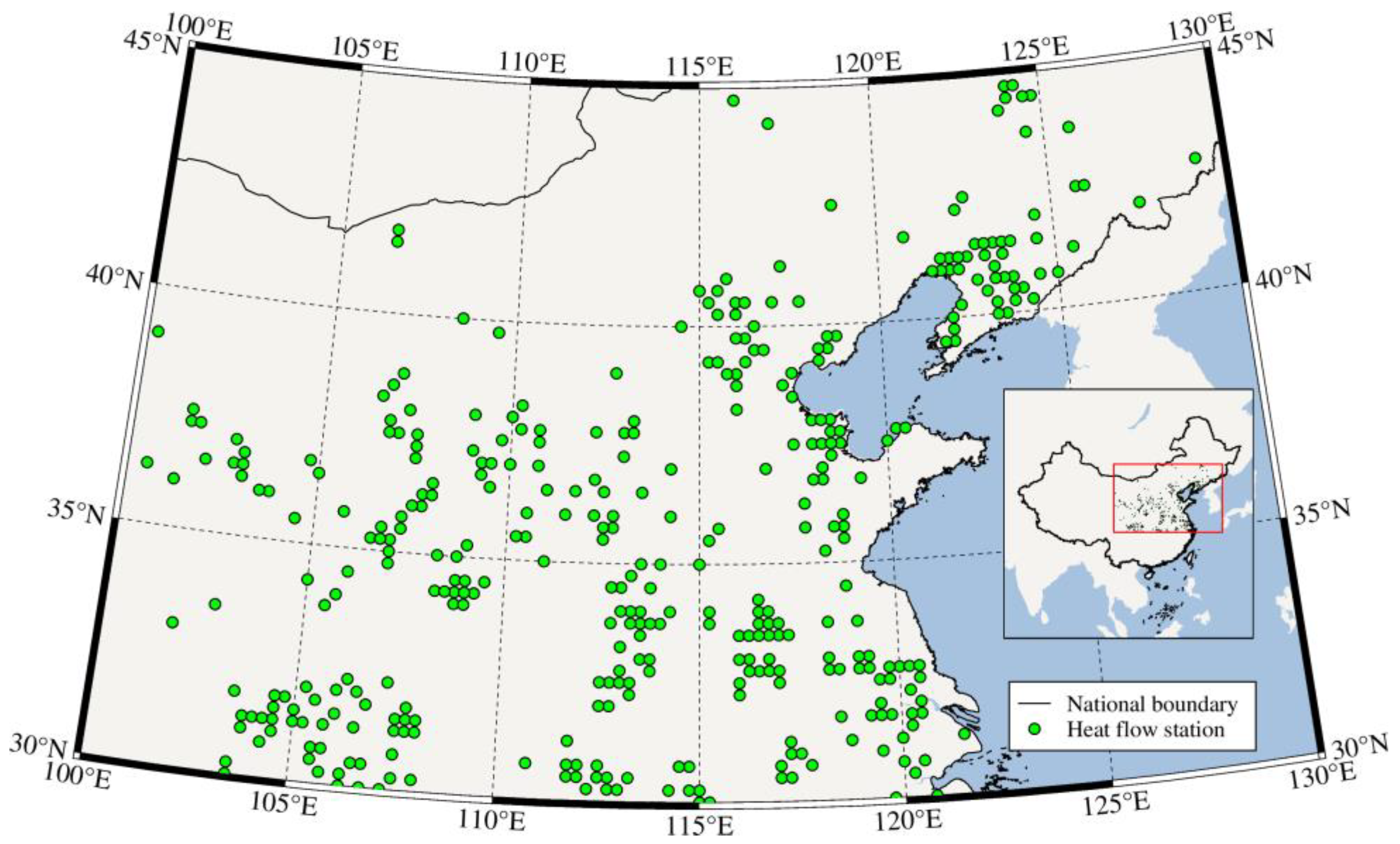
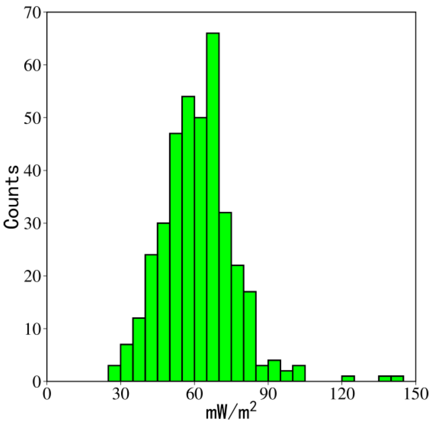
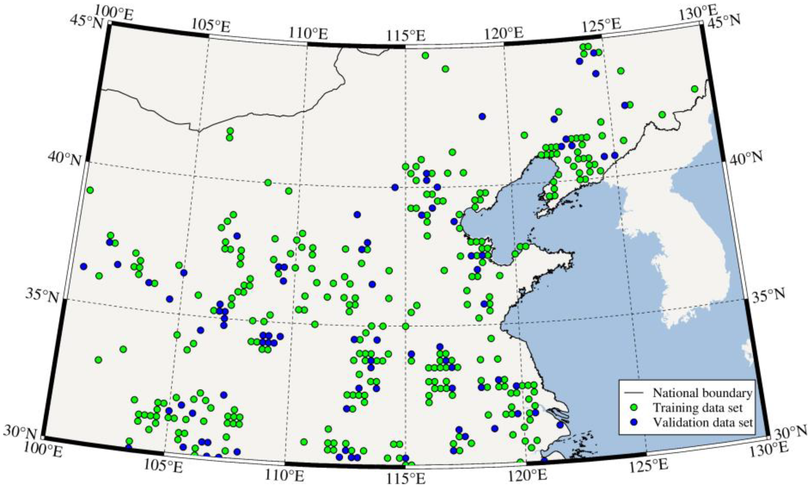
2.1. Geothermal Heat Flow

We integrated all the published heat flow data which included 1230 heat flow measurements in China [10,11,12]. Among them, 716 measurements were located in the NCC. After dividing and averaging them onto a 0.25°× 0.25° grid, the final number of data points was 379. The data distribution is shown in Figure 1. Generally, the data distribution was uneven, with dense measurements in the south and eastern coastal areas and sparse measurements in the western and northern areas. The histogram in Figure 2. shows that the heat flow in the study area had a maximum value of 140.7 mW/m², and a minimum value of 26.4 mW/m², with an average value of 61.5 mW/m².

2.2. Geological and Geophysical Information

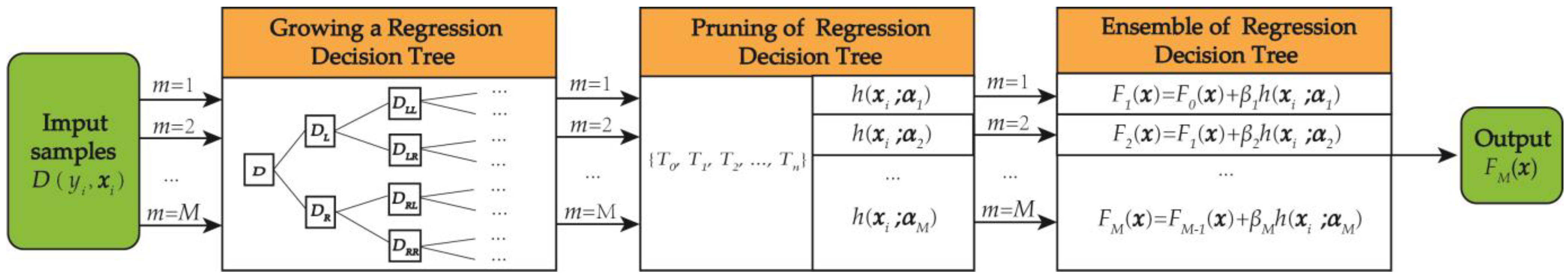
The use of reliable data was crucial for the prediction results, with the first step being determination of the features to be used [8]. In the process of constructing the GBRT prediction model, we selected 12 features (

Table 1. The geophysical and geological features used in this study with their respective sources.

	Feature	Publication
1	Distance to hotspot	Anderson (2016)
2	Upper crustal thickness	Laske et al. (2013)
3	Moho temperature	Xia et al. (2020)
4	Topography	Smith et al. (1997)
5	Distance to volcano	Goutorbe et al. (2011)
6	Thermal lithosphere thickness	Xia et al. (2020)
7	Upper mantle density anomaly	Laske et al. (2013)
8	Crustal thickness	Laske et al. (2013)
9	Depth to Moho	Laske et al. (2013)
10	Mid-crustal thickness	Laske et al. (2013)
11	Bougeur gravity anomaly	Sandwell et al. (2014) and Pavlis et al. (2012)
12	Magnetic anomaly	Maus et al. (2009)

) with strong relation to the geothermal heat flow to participate in the training. Among them, the Bouguer gravity anomaly is inferred from the Global Ocean Gravity Model [13] and the EGM2008 model [14]. The Global Ocean Gravity Model was constructed by combining the new radar altimeter measurements from the CryoSat-2 and the Jason-1 satellites. The EGM2008 model was constructed using the GRACE satellite tracking data (ITG-GRACE03S position coefficient information and corresponding covariance information), the satellite altimetry data, and the ground gravity data. The magnetic anomaly data were derived from the satellite aeromagnetic data [15]. The upper crustal thickness, the mid-crustal thickness, the crustal thickness, the upper mantle density, and the Depth to Moho data were all from CRUST1.0 [16], a global 3D crustal model constructed from seismic wave velocities, which has higher accuracy and resolution than the previous CRUST5.1 [17] and CRUST2.0 [18] models. The topographic relief data were referenced by combining the existing depth soundings with the high-resolution ocean gravity information from the Geosat and the ERS-1 spacecraft to produce the digital ocean bathymetry maps with horizontal resolution of 1 to 12 km [19]. For the Moho temperature and the thermal lithosphere thickness, we used the result of Xia et al. (2020) [3]. We selected the ten most typical volcanoes in China [20]. The locations of the hotspots were from Anderson (2016) [21]. These geophysical and geological features were processed in the same way as the geothermal heat flow data, and the above data were interpolated onto a 0.25° × 0.25° grid. In addition, for the volcanoes and the hotspots, we added the distance from the data points to the nearest volcano and hotspot as features for training.

3. Method

The GBRT prediction method does not completely depend on the number and the spatial distribution of the measured heat flow values, and there have been many successful applications in the heat flow prediction [7,8,9]. Therefore, in this study, we choose the GBRT method to predict the heat flow in the NCC. The GBRT is a supervised machine learning method initially proposed by Friedman (2001), which is a strong learner weighted by the ensemble of multiple weak learners [4,22]. Each weak learner is an individual regression decision tree, and each subtree learns in the direction of the negative gradient of the residuals of the previous tree. By iterating continuously to reach the minimum value of the loss function, the GBRT prediction model is constructed. The algorithm mainly includes the growing of regression decision trees, pruning of regression decision trees, and the ensemble of regression decision trees.

3.1. Growing a Regression Decision Tree

Growing a regression decision tree is mainly based on the minimum mean square deviation, finding the best split variable j and the split point d in the training sample set D, and then recursively constructing the binary tree [23]. The split variable j represents the jth feature. The splitting point d is the splitting position with the minimum mean square error when splitting according to the jth feature. The training sample set [4] is:

$$D=\left\{{(y}_1{,x}_1{),(y}_2{,x}_2{),\text{…},(y}_N{,x}_N)\right\}$$

(1)

where x_i is the input variable, and y_i represents the corresponding label, in which i = 1, 2, ..., N.

First, a feature is selected to sort N training samples by the feature value, and then the training samples are divided into two subsets, D_L and D_R, by using the feature value from the smallest to the largest as the split point. The optimal split pair (j, d) is solved by [23]

$$\underset{j,d}{\mathit{min}}\left[\underset{c_1}{\mathit{min}}\sum _{x_i\in D_L (j,d)}{\left(y_i-c_L\right)}^2+\underset{c_2}{\mathit{min}}\sum _{x_i\in D_R (j,d)}{\left(y_i-c_R\right)}^2\right]$$

(2)

where c_L represents the average value of all y in the left subset D_L, and c_R stands for the average value of all y in the right subset D_R. The optimal split result under the feature is determined by minimizing the squared error. Finally, all features are traversed, and the above process is repeated to obtain the optimal split variable j and the optimal split point d.

Then we continue to cut the left and right subsets D_L and D_R in the same way and increase the branches of the regression decision tree until the conditions are met so as to generate an unpruned regression decision tree f (x) [22]

$$f\left(x\right)={{\displaystyle \sum }}_{ r=1}^{ K}{c}_{r}I (x\in D_r)$$

(3)

Each subset is a feature unit, and each feature unit has a fixed output value c_r, which is the label mean of the corresponding subset D_r.

3.2. Pruning of Regression Decision Tree

In order to make the structure of the regression decision tree as simple as possible and to prevent overfitting, it needs to be pruned without loss of accuracy. Equation (4) is often used as an evaluation criterion for pruned subtrees [23,24]:

$$C_{\alpha }\left(T\right)=C\left(T\right)+\alpha \left|T\right|$$

(4)

where C(T) represents the mean square error of the node sample set; |T| is the number of leaf nodes in subtree T; α is a parameter used to balance the data fitting and complexity of the model:

$$\alpha =\frac{C\left(T\right)-{C(T}_t)}{{|T}_t|-1}$$

(5)

where t is any node inside a generated regression decision tree, and T_t is the subtree with t as the root node.

After the value of α is calculated by Equation (5), the node with the smallest value of α is pruned to obtain the new subtree after one pruning. The above process is repeated until the root node is left, and then a sequence of regression decision trees {T₀, T₁, T₂, …, T_n} is obtained, where T₀ is the initial unpruned regression decision tree. Finally, the subtree with the smallest evaluation criteria C_α(T) is selected as a complete regression decision tree in the decision tree sequence.

3.3. Ensemble of Regression Decision Trees

After pruning the regression decision tree, it is possible to learn based on its residuals, and then integrate the regression decision tree to obtain a strong learner. Firstly, the strong learner F₀ (x) is initialized with the mean square error as the loss function L [4,25]:

$$F_0{\left(x\right)=\mathit{argmin}}_{\beta }{{\displaystyle \sum }}_{i=1}^N{L(y}_i ,\beta )$$

(6)

where N represents the number of training samples, and β is the coefficient of the weak learner. Equation (7) calculates the negative gradient value of the loss function with F(x) as a variable after each iteration, which is the negative derivative value $\widetilde{y_i}$ of the loss function at F_m-1 (x). The value of m is 1, 2, ..., M. M is the total number of regression trees.

$$\widetilde{y_i}=-{\left[\frac{\partial {L(y}_{i ,}{F(\mathbf{x}}_i\left)\right)}{\partial {F(\mathbf{x}}_i)}\right]}_{{F\left(\mathbf{x}\right)=F}_{m-1}\left(\mathbf{x}\right)}i=1, N$$

(7)

After each training session, the optimal solution α_m of the parameters is solved by the negative gradient value $\widetilde{y_i}$ and the current trained regression decision tree h (x_i; α) [4].

$${\mathit{\alpha }}_m{=\mathit{argmin}}_{\alpha ,\beta }{{\displaystyle \sum }}_{ i=1}^{ N}\left[ \widetilde{y_i}-{\beta h(\mathit{x}}_i ;\alpha )\right]$$

(8)

Subsequently, execute the line search of the steepest descent method to solve the coefficient β_m of the regression decision treen [4]:

$${\beta }_m{=\mathit{argmin}}_{\beta }{{\displaystyle \sum }}_{i=1}^N{L(y}_{i }{,F}_{m-1}{(\mathit{x}}_i{)+\beta h(\mathit{x}}_i{ ;\mathit{\alpha }}_m\left)\right)$$

(9)

In this way, an iteration is completed. Subsequently, the regression decision tree is updated according to the regression decision tree obtained from the iteration, which is the last result added to the next iteration:

$$F_m{\left(\mathit{x}\right)=F}_{m-1}{\left(\mathit{x}\right)+\beta }_m{h(\mathit{x} ;\mathit{\alpha }}_m)$$

(10)

By repeating the above process and iterating for M times, the GBRT strong learner prediction model integrated by M regression decision trees is obtained. The overall process of the GBRT algorithm is summarized in Figure 3.

4. Results

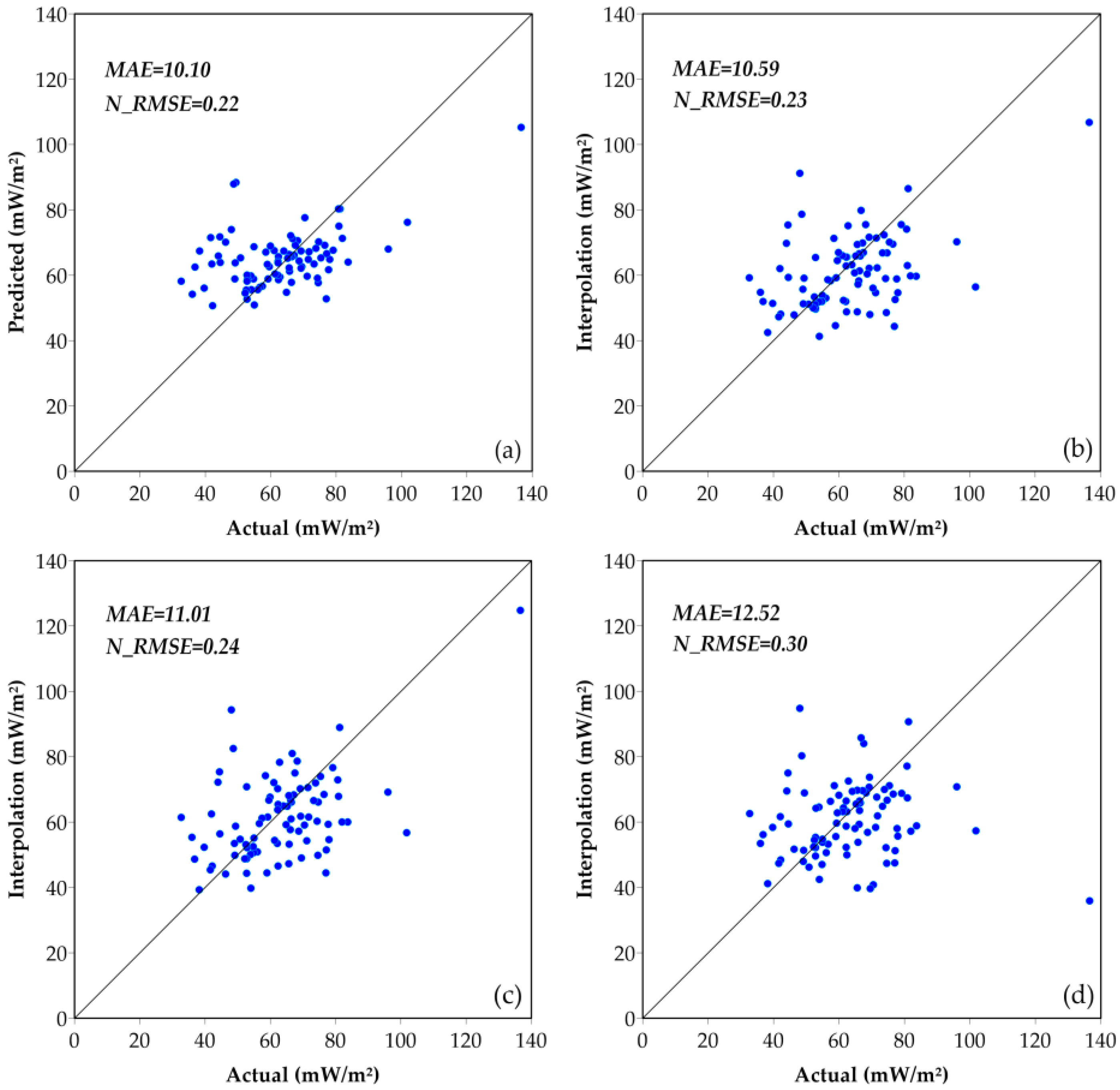
4.1. Prediction Performance Analysis

We randomly divided the 379 geodetic heat flow data samples in the NCC region into two data sets, of which 80% of the data volume was used as the training set and the remaining 20% as the validation set (Figure 4). Assuming that the heat flow values at the locations of the data points in the validation set were unknown, the remaining 20% of the heat flow data were predicted using four methods based on the training data set, namely the GBRT, the kriging interpolation, the minimum curvature interpolation and the 3D interpolation. Finally, the obtained results were compared and analyzed with the observed values in the validation set.

In order to assess the accuracy of the heat flow prediction, the uncertainty of the prediction results was quantified by using mean absolute error (MAE), and normalized mean square error (N_RMSE). MAE represents the average of the absolute values of the deviation of all individual observations from the arithmetic mean, with smaller values representing a smaller deviation of the data values from the mean; N_RMSE is a simplified transformation of the expression of mean square error. The value is between 0 and 1, with smaller values representing smaller errors. The calculations of MAE and N_RMSE are shown in Equations (11) and (12) [26], respectively:

$$\mathit{MAE}=\frac{1}{n}{{\displaystyle \sum }}_{ 1}^{ n}{|y}_i-\widehat{y_i}|$$

(11)

$$\mathit{N}\mathit{\text{\_}}\mathit{RMSE}=\frac{1}{ y \text{¯}}\sqrt{ \frac{1}{n}{{\displaystyle \sum }}_{ 1}^{ n}{{(y}_i-\widehat{y_i} )}^2}$$

(12)

where y_i is the ith heat flow observation value in the validation set, $\overline{y}$ is the average heat flow observation value in the validation set, $\widehat{y_i}$ is the ith heat flow predicted value in the validation set, and n is the number of heat flow observed in the validation set.

The results of the linear correlation analysis between the heat flow measurements in the validation set and the predicted values of the four methods; the GBRT, the kriging interpolation, the minimum curvature interpolation, and the 3D interpolation; are shown in Figure 5. The average absolute errors (MAE) of the GBRT, the kriging interpolation, the minimum curvature interpolation and the 3D interpolation methods are 10.10, 10.59, 11.01 and 12.52, respectively, showing an increase of errors. The normalized mean square error (N_RMSE) was 0.22, 0.23, 0.24 and 0.30, respectively, which also indicated an increase in errors. The difference between the maximum value and the minimum value was 0.08. It is obvious that the GBRT had the best predictive performance among the four methods, while the 3D interpolation showed the worst performance.

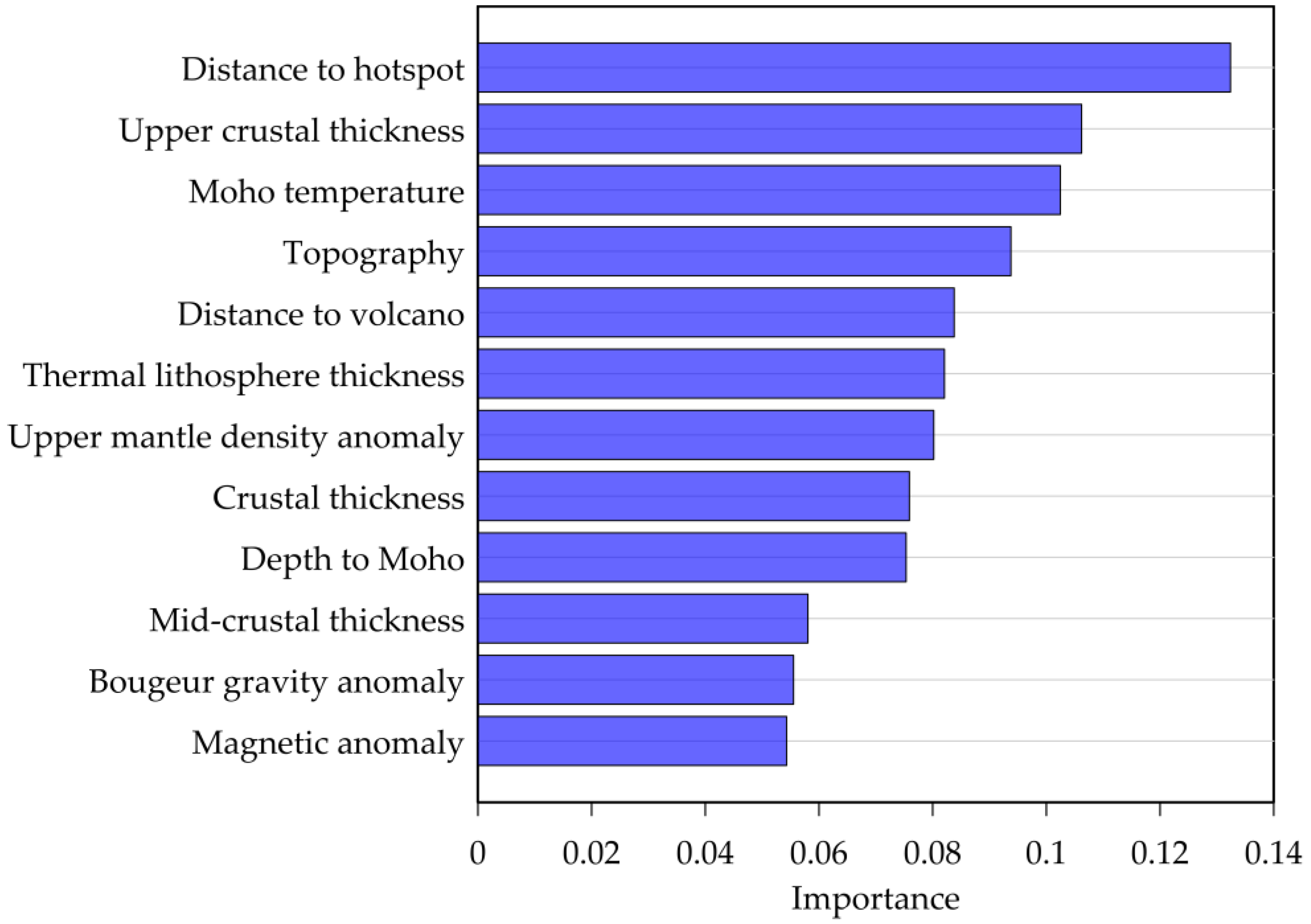
4.2. Calculating Feature Importance

The geological and the geophysical information features used in this study were carefully selected during the training of the samples based on the calculation of importance (Figure 6). The importance of each feature is the magnitude of the effect of each feature component on the classification or the regression, and is calculated by summing up the splitting mass of each feature in the decision tree. Since this study is a regression problem, the splitting mass is the decreasing value of the regression error for each split. The calculation is a cumulative summation of the splitting masses of each feature component in the decision tree. The sum of the splitting masses of the sth feature component is assumed to be q_s, and the splitting masses are normalized after summing up the feature components as follows [4]:

$$\omega =\frac{q_s}{{{\displaystyle \sum }}_{ s=1}^{ p}{q}_s}$$

(13)

where w represents the importance of each feature and p represents the dimensionality of the feature vector. The larger the value, the greater the importance of the corresponding feature, and the greater the contribution of the corresponding feature to the regression.

The correlation between the 12 geological and geophysical features and the geothermal heat flow was different. The distance to hotspot had the highest weighting of 0.13, thus it had the strongest correlation with the geothermal heat flow. The thickness of the upper crust and the Moho temperature also showed a strong correlation with a weighting of 0.11 and 0.10, respectively. Since the heat flow measurements were relatively distant from the craters [27,28,29,30,31], the distance to the volcano only showed a small weight value of 0.08 in this study. Two geophysical features, the Bouguer gravity anomaly and the satellite aeromagnetic anomaly, had the weakest correlation with the geothermal heat flow, with feature weights of 0.06 and 0.05, respectively, indicating that the two parameters, the density and the magnetization, were less intrinsically linked to the geothermal heat flow. The weight share and the ranking of each geological and geophysical feature are shown in Figure 6.

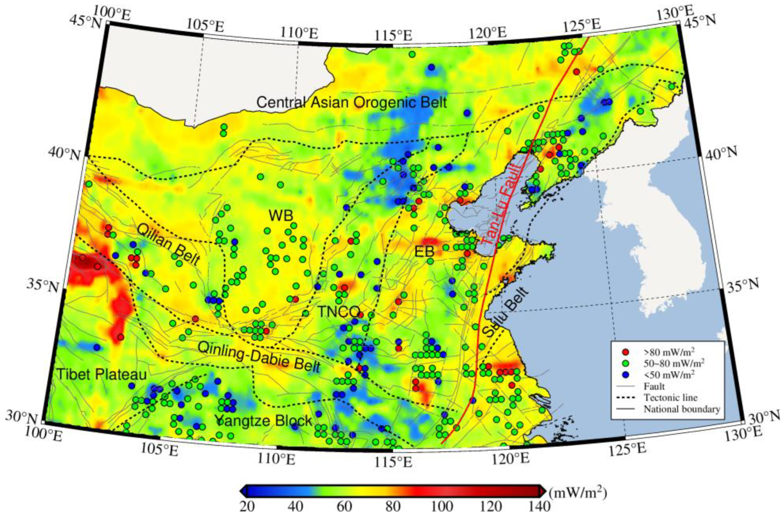
4.3. Predicting NCC Heat Flow

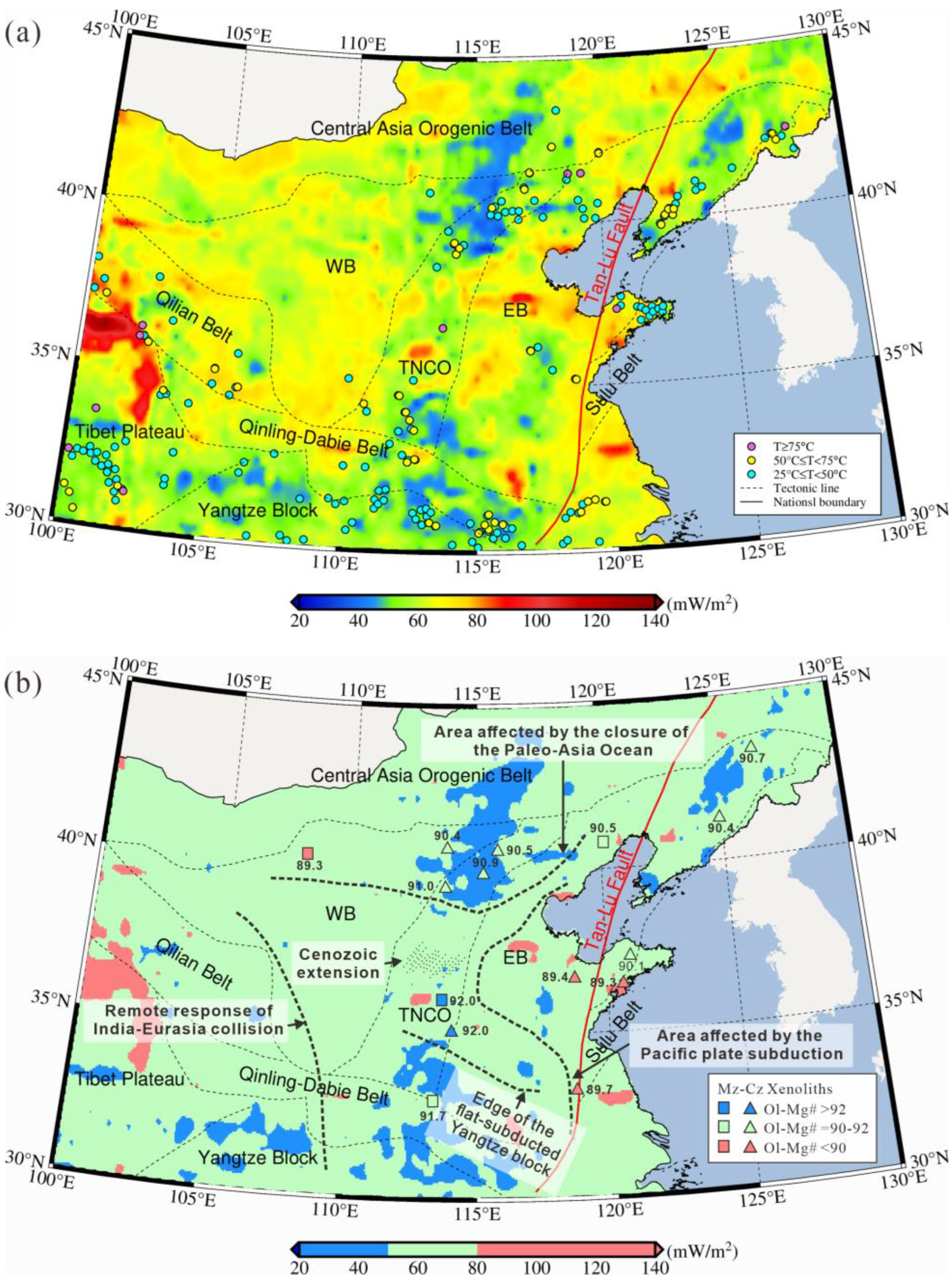
The heat flow map with a resolution of 0.25° was obtained in the NCC by the GBRT prediction model developed in this study, as shown in Figure 7. The 379 heat flow observations were divided into three intervals: >80 mW/m², 50~80 mW/m², and <50 mW/m², corresponding to the red, green, and blue dots in Figure 7, respectively. Figure 7 shows that the predicted heat flow values agreed well with the observations. The heat flow in the study area was in the range of 50–80 mW/m². Generally, the heat flow values in the eastern coastal area of the NCC and the northeastern Tibet Plateau were higher than those in the central part. The highest heat flow value was located in the northern part of the Tibet Plateau, with a value of 133 mW/m². Several relatively scattered and small-scale regions with high heat flow are located in the central part of Trans-North China Orogenic Belt (TNCO), the Eastern Block and the southeastern Sulu Belt, with heat flow values greater than 80 mW/m². The low heat flow areas were mainly distributed in the eastern Qinling-Dabie Belt, the Yangtze Block and on the boundary of the TNCO and Central Asian Orogenic Belt, with heat flow values of less than 50 mW/m². The lowest value was about 26 mW/m², which appeared in the northwestern part of Yangtze Block.

5. Discussion

Although the observation points of heat flow within the study area were sparse and extremely unevenly distributed, we still obtained plausible heat flow values under the constraints of the 12 geological and geophysical features. The GBRT has been shown to outperform the kriging interpolation, the minimum curvature interpolation, and the 3D interpolation in the prediction performance analysis. The major difference between the GBRT and the interpolation is that multiple geological and geophysical information features can be used to constrain the prediction of the GBRT, which fully takes into account the tectonic background of the study area. The heat flow map obtained from the kriging interpolation in Xia et al. 2020 showed a narrow band of high heat flow concentration extending from the central and northern Tibetan Plateau, through the southeastern WB, across the central TNCO to the EB, with heat flow values of 70–90 mW/m². This agrees well with our predication.

The temperature of hot springs is a direct indication of the geothermal heat flow [35,36,37,38,39,40]. To evaluate the accuracy of our prediction results, we studied the distribution of hot springs by dividing the regions of hot springs into three intervals based on their temperature: the high-temperature hot springs (T ≥ 75 °C), the medium-temperature hot springs (50 °C ≤ T < 75 °C), and the low-temperature hot springs (25 °C ≤ T < 50 °C) [38] (Figure 8a). The hot springs in the study area were mainly medium- and low-temperature hot springs with temperatures less than 75°C. Only a few hot springs showed temperatures of greater than 75 °C. We found that the distribution of hot springs showed a certain regularity, with medium- to low-temperature hot springs mainly exposed in areas of low heat flow in the central north and south of the study area, while the high-temperature hot springs are exposed in areas with higher heat flow values. This verified the robustness of our prediction model.

To further analyze the characteristics of the high and low heat flow concentration regions, we simplified the heat flow map by dividing the study area into regions with heat flow values of <50 mW/m², 50–80 mW/m², and >80 mW/m² as shown in Figure 8b. We found that in the two low-heat-flow regions in the northern TNCO and the junction area of southern TNCO and EB were of low lithospheric mantle density (<3.33 g/cm³) [3], with olivine-Mg# roughly between 90 and 92. In contrast, there were several scattered high heat flow regions (red regions in Figure 8b) in the southeast coastal area of the EB with lithospheric mantle density of 3.37–3.39 g/cm³ [3] and olivine-Mg# of less than 90.

Due to the remote response of the collision of the Cenozoic Indian plate with the Eurasian plate in the western part of the NCC, the overall elevation in and around the Tibetan Plateau was uplifted. The thickness of the thermal lithosphere in these regions was relatively thin compared to its surrounding areas [38]. The southeastern coastal area was subjected to the Mesozoic subduction of the Paleo-Pacific plate underneath the Eurasian plate [3]. The heat flow in the above two regions (the red regions in Figure 8b) was high (>80 mW/m²) and the olivine-Mg# was low (<90), indicating that they had been severely reworked during the long-term plate activity, and that the original lithospheric mantle components had been strongly modified compared with the surrounding areas [3,41]. As a result, the degree of fracture/fault development was significantly high, which provided the conditions for the formation of heat-conducting channels. The heat from the Earth’s interior was transported upward along the channels, producing high heat flow values at the surface. Correspondingly, the high-temperature hot springs and the medium-to-low-temperature hot springs were concentrated in the area of high heat flow values. Although the northern part of the TNCO is influenced by the Paleozoic closure of the Paleo-Asian Ocean, and the Qinling-Dabie orogen is influenced by the Triassic subduction of the Yangtze Block, the heat flow values in these regions were relatively low, with relatively high olivine-Mg# (90–92). The degree of the fracture/fault development was also relatively low. As a result, these areas were relatively intact. Only several small-scale high heat flow areas appeared in the central part of the TNCO due to the influence of the Cenozoic extensional tectonics.

Due to the scarce distribution of heat flow measurements in Greenland and Antarctica, the Gaussian kernel function was used to supplement the sample set [7,8]. In North China, the data coverage had reached two thirds of the study area, thus it was not necessary to supplement the sample set. It is generally accepted that interpolation methods are highly dependent on the quantity and the spatial distribution of heat flow measurements, which were major challenges for previous heat flow maps in mainland China [1]. The comparison of the predicted heat flow map with the plate tectonics, the olivine-Mg#, and the hot spring distribution in North China has justified the prediction from the GBRT method.

6. Conclusions

In this study, a new heat flow map of North China was obtained by the GBRT method. The prediction performance analysis result showed that this heat flow map was more reasonable than those derived from the kriging interpolation, the minimum curvature interpolation and the 3D interpolation methods. The new heat flow map of the NCC elucidates the intrinsic relationship between the geothermal heat flow and the plate tectonics, the olivine-Mg#, and the hot spring distribution.

We found that the eastern margin of the Tibet Plateau and the eastern coastal areas were of high geothermal heat flow, which were affected by the collision of the Cenozoic Indian plate to the Eurasian plate and the subduction of the Mesozoic Pacific plate underneath the Eurasian plate, respectively. The NCC was largely destructed, with fractures developed to form heat-conducting channels, showing high terrestrial heat flow values and high temperatures of exposed hot springs. Conversely, the northern part of the TNCO and the southmost NCC exhibited low heat flow values due to a low degree of lithospheric modification and less fault/fracture development, where only the medium and the low temperature hot springs were exposed.

By comparing the predicted heat flow map and the location of heat flow observations in North China, we found that the GBRT could still obtain a reliable result under the constraint of geological and geophysical information in the region where the observations were scarce and unevenly distributed. The regions of different heat flow values mentioned above possessed only some discontinuous and scattered heat flow observation points, but still showed reasonable heat flow patterns consistent with the plate tectonics, the olivine-Mg#, and the hot spring distribution. The high heat flow values obtained in the study area provide effective indicators for the development of geothermal energy in China. This is the first terrestrial heat flow map derived from machine learning method in North China, using multiple geological and geophysical datasets. From a global perspective, the global heat flow distribution can be supplemented and the global heat flow resolution can be improved.

References

1. Jiang, G.Z.; Hu, S.B.; Shi, Y.Z.; Zhang, C.; Wang, Z.T.; Hu, D. Terrestrial heat flow of continental China: Updated dataset and tectonic implications. Tectonophysics 2019, 753, 36–48. [Google Scholar] [CrossRef]
2. Demirbas, A.H. Global geothermal energy scenario by 2040. Energy Sources Part A 2008, 30, 1890–1895. [Google Scholar] [CrossRef]
3. Xia, B.; Thybo, H.; Artemieva, I.M. Lithosphere Mantle Density of the North China Craton. J. Geophys. Res. Solid Earth 2020, 125, e2020JB020296. [Google Scholar] [CrossRef]
4. Friedman, J.H. 1999 Reitz lecture greedy function appoximation: A gradient boosting machine. Ann. Stat. 2001, 29, 1189–1232. [Google Scholar]
5. Persson, C.; Bacher, P.; Shiga, T.; Madsen, H. Multi-site solar power forecasting using gradient boosted regression trees. Sol. Energy 2017, 150, 423–436. [Google Scholar] [CrossRef]
6. Deng, L.; Yang, W.; Liu, H. PredPRBA: Prediction of Protein-RNA Binding Affinity Using Gradient Boosted Regression Trees. Front. Genet. 2019, 10, 637. [Google Scholar] [CrossRef]
7. Rezvanbehbahani, S.; Stearns, L.A.; Kadivar, A.; Walker, J.D.; Van der Veen, C.J. Predicting the Geothermal Heat Flux in Greenland: A Machine Learning Approach. Geophys. Res. Lett. 2017, 44, 12271–12279. [Google Scholar] [CrossRef]
8. Lösing, M.; Ebbing, J. Predicting Geothermal Heat Flow in Antarctica With a Machine Learning Approach. J. Geophys. Res. Solid Earth 2021, 126, e2020JB021499. [Google Scholar] [CrossRef]
9. Wang, L.; Zhang, Y.; Yao, Y.; Xiao, Z.; Shang, K.; Guo, X.; Yang, J.; Xue, S.; Wang, J. GBRT-Based Estimation of Terrestrial Latent Heat Flux in the Haihe River Basin from Satellite and Reanalysis Datasets. Remote Sens. 2021, 13, 1054. [Google Scholar] [CrossRef]
10. Wang, J.Y.; Huang, S.P. Compilation of heat flow data in the continental area of China (2th edition). Seismol. Geol. 1990, 12, 351–366. [Google Scholar]
11. Hu, S.B.; He, L.J.; Wang, J.Y. Compilation of heat flow data in the continental area of China (3th edition). Chin. J. Geophys. 2001, 44, 142–157. [Google Scholar] [CrossRef]
12. Jiang, G.Z.; Gao, P.; Rao, S.; Zhang, L.Y.; Tang, X.Y.; Huang, F.; Zhao, P.; Pang, Z.H.; He, L.J.; Hu, S.B.; et al. Compilation of heat flow data in the continental area of China (4th edition). Chin. J. Geophys. 2016, 59, 2892–2910. [Google Scholar] [CrossRef]
13. Sandwell, D.T.; Muller, R.D.; Smith, W.H.; Garcia, E.; Francis, R. Marine geophysics. New global marine gravity model from CryoSat-2 and Jason-1 reveals buried tectonic structure. Science 2014, 346, 65–67. [Google Scholar] [CrossRef] [PubMed]
14. Pavlis, N.K.; Holmes, S.A.; Kenyon, S.C.; Factor, J.K. The development and evaluation of the Earth Gravitational Model 2008 (EGM2008). J. Geophys. Res. Solid Earth 2012, 117, 1–38. [Google Scholar] [CrossRef]
15. Maus, S.; Barckhausen, U.; Berkenbosch, H.; Bournas, N.; Brozena, J.; Childers, V.; Dostaler, F.; Fairhead, J.D.; Finn, C.; von Frese, R.R.B.; et al. EMAG2: A 2-arc min resolution Earth Magnetic Anomaly Grid compiled from satellite, airborne, and marine magnetic measurements. Geochem. Geophys. Geosyst. 2009, 10, 1–12. [Google Scholar] [CrossRef]
16. Laske, G.; Masters, G.; Ma, Z.; Pasyanos, M. Update on CRUST1.0—A 1-degree Global Model of Earth’s Crust. Geophys. Res. Abstr. 2013, 15, 2658. [Google Scholar]
17. Mooney, W.D.; Laske, G.; Masters, T.G. CRUST 5.1: A global crustal model at 5° × 5°. J. Geophys. Res. Solid Earth 1998, 103, 727–747. [Google Scholar] [CrossRef]
18. Bassin, C. The current limits of resolution for surface wave tomography in North America. Eos Trans. Am. Geophys. Union 2000, 81, F897. [Google Scholar]
19. Smith, W.H.F.; Sandwell, D.T. Global Sea Floor Topography from Satellite Altimetry and Ship Depth Soundings. Science 1997, 277, 1956–1962. [Google Scholar] [CrossRef]
20. Goutorbe, B.; Poort, J.; Lucazeau, F.; Raillard, S. Global heat flow trends resolved from multiple geological and geophysical proxies. Geophys. J. Int. 2011, 187, 1405–1419. [Google Scholar] [CrossRef]
21. Anderson, D.L. The Complete Hot Spot. 2016. Available online: http://www.mantleplumes.org/CompleateHotspot.html (accessed on 29 August 2016).
22. Friedman, J.H. Stochastic gradient boosting. Comput. Stat. Data Anal. 2002, 38, 367–378. [Google Scholar] [CrossRef]
23. Li, B.; Friedman, J.; Olshen, R.; Stone, C. Classification and Regression Trees (CART). Biometrics 1984, 40, 358–361. [Google Scholar]
24. Frank, E. Pruning Decision Trees and Lists. Ph.D. Thesis, The University of Waikato, Waikato, New Zealand, 2000. Available online: https://hdl.handle.net/10289/14883 (accessed on 20 March 2022).
25. Natekin, A.; Knoll, A. Gradient boosting machines, a tutorial. Front. Neurorobot. 2013, 7, 21. [Google Scholar] [CrossRef]
26. Jifu, H.; Kewen, L.; Xinwei, W.; Nanan, G.; Xiaoping, M.; Lin, J. A Machine Learning Methodology for Predicting Geothermal Heat Flow in the Bohai Bay Basin, China. Nat. Resour. Res. 2022, 31, 237–260. [Google Scholar]
27. Fan, X.; Guo, Z.; Zhao, Y.; Chen, Q.F. Crust and Uppermost Mantle Magma Plumbing System Beneath Changbaishan Intraplate Volcano, China/North Korea, Revealed by Ambient Noise Adjoint Tomography. Geophys. Res. Lett. 2022, 49, e2022GL098308. [Google Scholar] [CrossRef]
28. Sun, Q.; Jackson, C.A.L.; Magee, C.; Xie, X. Deeply buried ancient volcanoes control hydrocarbon migration in the South China Sea. Basin Res. 2019, 32, 146–162. [Google Scholar] [CrossRef] [Green Version]
29. Wan, Z.; Wang, X.; Lu, Y.; Sun, Y.; Xia, B. Geochemical characteristics of mud volcano fluids in the southern margin of the Junggar basin, NW China: Implications for fluid origin and mud volcano formation mechanisms. Int. Geol. Rev. 2017, 59, 1723–1735. [Google Scholar] [CrossRef]
30. Wei, W.; Hammond, J.O.S.; Zhao, D.; Xu, J.; Liu, Q.; Gu, Y. Seismic Evidence for a Mantle Transition Zone Origin of the Wudalianchi and Halaha Volcanoes in Northeast China. Geochem. Geophys. Geosyst. 2019, 20, 398–416. [Google Scholar] [CrossRef]
31. Weia, H.; Sparksb, R.S.J.; Liua, R.; Fana, Q.; Wanga, Y. Three active volcanoes in China and their hazards. J. Asian Earth Sci. 2003, 21, 515–526. [Google Scholar] [CrossRef]
32. Deng, Q.D.; Zhang, P.Z.; Ran, Y.K.; Deng, Q.; Zhang, P.; Ran, Y. Active tectonics and earthquake activities in China. Earth Sci. Front. 2003, 10, 66–73. [Google Scholar]
33. Deng, Q.D. Active Tectonic Map of China (1:4 Million); Seismological Press: Beijing, China, 2007. [Google Scholar]
34. Qu, C.Y. Building to the active tectonic database of China. Seismol. Geol. 2008, 30, 298–304. [Google Scholar] [CrossRef]
35. Chen, L. Concordant structural variations from the surface to the base of the upper mantle in the North China Craton and its tectonic implications. Lithos 2010, 120, 96–115. [Google Scholar] [CrossRef]
36. Jiang, S.C.; Li, S.W.; Wang, G.; Somerville, L.; Zhang, W.; Zhao, F.; Chen, H. Tectonic units of the Early Precambrian basement within the North China Craton: Constraints from gravitational and magnetic anomalies. Precambrian Res. 2018, 318, 122–132. [Google Scholar] [CrossRef]
37. Kusky, T.M. Geophysical and geological tests of tectonic models of the North China Craton. Gondwana Res. 2011, 20, 26–35. [Google Scholar] [CrossRef]
38. Qiu, N.S.; Tang, B.N.; Zhu, C.Q. Deep thermal background of hot spring distribution in the Chinese continent. Acta Geol. Sin. 2022, 96, 195–207. [Google Scholar] [CrossRef]
39. Wang, Y.; Zhou, L.; Liu, S.; Li, J.; Yang, T. Post-cratonization deformation processes and tectonic evolution of the North China Craton. Earth-Sci. Rev. 2018, 177, 320–365. [Google Scholar] [CrossRef]
40. Zhai, M. Precambrian tectonic evolution of the North China Craton. Geol. Soc. 2015, 226, 57–72. [Google Scholar] [CrossRef]
41. Zheng, J.; Xia, B.; Dai, H.; Dai, H.; Ma, Q. Lithospheric structure and evolution of the North China Craton: An integrated study of geophysical and xenolith data. Sci. China Earth Sci. 2020, 64, 205–219. [Google Scholar] [CrossRef]
Figure 1. Map of heat flow measurements in North China.
Energies 16 01620 g001
Figure 2. Histogram of heat flow values.
Energies 16 01620 g002
Figure 3. Flowchart of the GBRT algorithm, where D(yi, xi) represents the training sample. DL and DR is the left and right subset obtained by optimal splitting of D, respectively. DLL, DLR, DRL, and DRR are the left and right subsets obtained by further optimal splitting of DL and DR. {T0, T1, T2, …, Tn} signify the sequence of pruned regression decision trees. h (xi; α) is the subtree with the smallest evaluation criterion selected, and is also the regression decision tree of current training. αm stands for the parameter of the regression decision tree, βm represents the coefficient of the regression decision tree (m=1, 2, …, M), M denotes the number of regression trees, and FM(x) is the strong learner of the Mth iteration.
Energies 16 01620 g003
Figure 4. Distribution of the training and the validation data points.
Energies 16 01620 g004
Figure 5. The prediction performance of GBRT (a), kriging interpolation (b), minimum curvature interpolation (c), and 3D interpolation (d).
Energies 16 01620 g005
Figure 6. Relative importance of each feature on the trained predication model.
Energies 16 01620 g006
Figure 7. Heat flow prediction results with regional tectonics. The red solid line delineates the most significant fault in the NCC, the north-south trending Tan-Lu Fault. Gray solid lines indicate minor faults [32,33,34]. Black dashed lines indicate the boundaries of different tectonic units. WB: Western Block; TNCO: Trans-North China Orogenic Belt; EB: Eastern Block.
Energies 16 01620 g007
Figure 8. (a) Map of hot spring distribution with heat flow prediction results as a background, the colored circles represent hot springs with different temperature [36]. (b) Sketch map showing a simplified heat flow map based on our heat flow prediction results, with the olivine-Mg# of xenoliths inserted. Triangles and squares mark locations of Cenozoic and Mesozoic kimberlites, respectively. Numbers close to symbols mark the olivine-Mg# in the xenoliths and the color of the symbols shows the average olivine-Mg# in the xenoliths [3,41].
Energies 16 01620 g008