Article

A New Type in TRNSYS 18 for Simulation of Borehole Heat Exchangers Affected by Different Groundwater Flow Velocities

1
Inewa s.r.l., NOI Techpark Südtirol/Alto Adige, Via Alessandro Volta 13, 39100 Bolzano, Italy
2
Dipartimento di Ingegneria Civile Ambientale, Politecnico di Milano, Piazza L. da Vinci 32, 20133 Milano, Italy
3
EURAC Research, NOI Techpark Südtirol/Alto Adige, Via Alessandro Volta 13, 39100 Bolzano, Italy
*
Author to whom correspondence should be addressed.
Energies 2023, 16(3), 1288; https://doi.org/10.3390/en16031288
Submission received: 21 December 2022 / Revised: 12 January 2023 / Accepted: 20 January 2023 / Published: 25 January 2023
(This article belongs to the Special Issue Low Carbon Energy Technology for Heating and Cooling of Buildings)

Abstract

:
Heating ventilating air-conditioning (HVAC) systems have been increasingly widespread in Italy: they can exploit renewable energies, are energy efficient systems, do not directly consume fossil fuels, and in the post-pandemic era, have also been subject to incentive processes by the Italian government. In South Tyrol, subject to harsh climates in both the winter and summer seasons, ground-source heat pump (GSHP) systems can be an excellent solution for the air conditioning of buildings. Unfortunately, too often, the design of HVAC systems with borehole heat exchangers (BHEs) is not adequate, and therefore, an innovative and expeditious numerical solution is proposed. A new numerical element (named Type285), written in Fortran code, was developed for TRNSYS 18 and able to implement the main features of BHEs and the surrounding aquifer. Type285 was compared with numerical models present in the literature (using hydrogeological software such as MODFLOW) and validated with the experimental data. The demonstration of the exchanged energy increase between the BHE and subsoil due to the increase in the groundwater flow velocity was carried out and evaluated. The choice to simulate BHE in TRNSYS using Type285 can be a fast and advantageous solution for HVAC system design.

1. Introduction

Heating ventilating air-conditioning (HVAC) systems such as groundwater and air heat pump systems coupled to borehole heat exchangers (BHE) have been used increasingly because they are among the cleanest and most energy efficient heating/cooling systems for houses, multi-residential buildings, public offices, or farms [1,2,3,4,5,6]. Because of the incentives for these systems by the Italian government, often the design of ground source heat pump (GSHP) systems is not adequate and superficial. The numerical modeling of the BHE is essential for the good design of a GHSP system. The following manuscript provides a specific tool useful to simulate one or more BHEs installed in the subsoil. A vertical BHE consists of a borehole, containing a backfilling material (generally grout consisting of bentonite) able to seal off a U-shape pipe where a heat carrier fluid (usually water or antifreeze solution) is circulated. The depth of the borehole usually ranges between 70 and 150 m and the drilling diameter is between 0.075 and 0.15 m. The vertical geothermal probe consists of one single or double U-shape pipe or coaxial pipe. Depending on the energy needs of the building and on the heat pump size, the number of BHEs installed into the ground can vary. The BHE is coupled to the evaporator of the GSHP, allowing heat to be extracted from the ground and provided to the condenser element, which releases the heat into a secondary system, providing climatization to the building. During summer, the operation can be reversed: the heat is extracted from the building and injected into the ground [7]. Clearly the energy performance of GSHP systems strongly depends on the heat transfer between the soil and the BHE; this also affects the thermal condition of the aquifer surrounding the BHE, generating cold or warm thermal plumes downgradient of the vertical probe. Therefore, there is a need to simulate, by means of numerical or analytical models, the GSHP systems and to evaluate the energy performance and thermal impact on the subsoil.
Many efforts have been carried out to understand and formulate the heat transfer process in BHEs: analytical solutions [8,9,10,11,12] and numerical models based on FORTRAN language, resulting in several commercially available tools for the design simulation of the BHE [13]. Among them, the TRNVDST analytical model [14], coupled to the dynamic energy simulation software TRNSYS [15], is a widesly used and reliable code that is able to simulate the heat transfer process between the BHE and the ground as well as the thermal interaction among the different U-pipes [16]. De Rosa et al. [17,18] developed a new TRNSYS type implementing a borehole-to-ground model to reproduce the short-term dynamic performance of a BHE and validated the approach by comparing the results with the experimental data (for a step-test and under normal operating conditions) of a real GSHP system. Cazorla-Marìn et al. [19] adopted a similar approach to reproduce the dynamic behavior of a coaxial BHE and validated the results by comparing them with the experimental data derived from a dual source heat pump (DSHP) system. All of these studies related to TRNSYS software and most of the available energy tools such as EWS [20], EED [21], GLHEPRO [22] Pilesim [23], and Modelica [24] have assumed a pure heat conduction in the ground and have not considered the effects of groundwater flow on the performance of the GSHP system; otherwise, as Angelotti et al. demonstrated, this assumption is very limiting because the role of the groundwater flow is essential and can improve the energy performance of a BHE up to 105% for a high flow velocity case [25].
In the hydrogeology field, a lot of computer software can accurately simulate the flow and mass transport according to different hydrogeological settings by exploiting finite difference (FD) or finite element (FE) approaches: FEFLOW, MODFLOW/MT3DMS, MODFLOW-USG, COMSOL, etc. In these software, the possibility of introducing the numerical element of the BHE into the subsoil or reproducing it through grid discretization is present. For instance, a FE algorithm was implemented in FEFLOW software [26] and the BHE was simulated by a set of one-dimensional finite-element representations [27]. The efficiency of BHE systems assuming different physical and thermal conditions was discussed and showed different heat transfer in an aquifer due to advection or dispersion phenomena [28]. Among the FD software, MT3DMS [29] was not explicitly designed to simulate heat transport, although temperature can be simulated as one of the species by entering appropriate transport coefficients, as carried out in [25]. The actual version of MODFLOW/MT3DMS is MODFLOW-USG [30,31], which is able to couple the flow numerical simulations to the heat transport modeling in an aquifer. Antelmi et al. [32] developed a numerical model of a single BHE using the connected linear network (CLN) package and showed how the approach results are smart and more expeditious than the usual BHE models; the approach was also verified and validated against numerical solutions with different hydrogeology settings and modeling grids in a thermal response test (TRT) application [33]. Furthermore, different authors [9,10,25,34,35] have also used numerical modeling to demonstrate the influence of the groundwater flow velocity on energy performance: they discussed how the variation in the Peclet number, directly proportional to groundwater flow velocity, and thermal diffusion could cause a different energy performance of the BHE system. All of the numerical modeling results were robust because they were compared with analytical solutions [36,37] or experimental data [3]. Alberti et al. [3] showed the experimental data of a GSHP system used for a particular field of application: air conditioning of a post-weaning piglet room at the Veterinary University of Lodi; they monitored different parameters such as the inlet and outlet fluid temperature of the BHE, the electricity consumed, and thermal power generated by the system.
From the previous analysis of the literature, it is clear that it is important to learn the thermal and hydrogeological features of the subsoil, allows for an understanding of the groundwater flow velocity, which influences the GSHP performance. From the point of view of hydrogeological software, the topic is clear and well-reproduced, but from the energy software, typically used by energy designers of HVAC systems, the role of groundwater is often neglected. Wang et al. [38] measured the heat extraction rate of a BHE in the presence of a groundwater flow deduced by the vertical temperature profile in the ground and simulated the process through TRNSYS software, usually applied to the energy design of air-climatization systems. No scientific publications implementing the groundwater flow issue coupled to BHE operation for HVAC system design using TRNSYS software are present in the literature. In TRNSYS, there is a specific element named “type” (which is a numerical element written in FORTRAN), which is able to simulate the BHE element and its behavior: TRNSYS Type280, developed by Pahud [39], is able to reproduce the U-shape pipe buried in an aquifer. This type was based on the TRNVDSTP model and is available just for TRNSYS 16 and does not work on the latter TRNSYS version (18).
The main aim of the present study was to create a new type (named Type285) for BHE systems in TRNSYS 18 starting from Type280 and improving it by introducing the possibility of setting different groundwater flow velocities coupled to different hydrogeological settings. This topic was the heart of a Fusion Grant project where a numerical modeling of a dual source heat pump (DSHP) system, based on groundwater and air as energy sources, was implemented and the control logics of the entire system were optimized thanks to the numerical model. As soon as the code of the Type285 was written and compiled, several numerical models were developed in TRNSYS with the aim to reproduce the identical BHE operation simulated in MODFLOW/MT3DMS and compare the exchanged energies in the aquifer. Furthermore, the possibility of implementing more than one BHE through Type285 was evaluated. A validation process of the type was carried out by comparing the results of TRNSYS models with experimental data [3]: the TRNSYS results agreed with MODFLOW/MT3DMS and demonstrated a large increase in the extracted or injected energy performance of the BHE when the groundwater flow velocity passed from 0 to 0.8 m/day. The results proved the capacity of this tool to be an efficient approach for scientists and technicians to design GSHP systems when an important groundwater flow is present in the subsoil.

2. Numerical Modeling Approach

2.1. Fusion Grant Project

The Fusion Grant project is a research project funded by Stiftung Südtiroler Sparkasse—Fondazione Cassa di Risparmio di Bolzano in 2021, where the research center “EURAC Research” and the company “Inewa s.r.l.” collaborated to improve the energy efficiency of a dual source heat pump (DSHP) system and promote their use in South Tyrol for air-climatization and domestic hot water preparation in residential buildings. The DSHP system has the advantage of combining two different sources (ground and external air) to optimize the energy performance and electric consumption of the system. The focus of the project was to create a smart control logic for the DSHP system installed in a HVAC system of a reference building. To reach this aim, detailed numerical modeling needed to be developed in TRNSYS to study the different energy scenarios. The central element of this numerical modeling was the reproduction of the geothermal source led by the BHE element. The present study describes all of the steps for the correct modeling of the BHE system in TRNSYS software (version 18). In previous versions of TRNSYS, a type (Type280) able to simulate BHE buried in an aquifer was already available: it correctly simulated the conduction processes, but the advection processes (due to groundwater flows) were not detailed nor validated. The simplification was too strong because the energy performance of the system could increase up to 100%, thus varying the groundwater flow velocity, as demonstrated in Angelotti’s [25] work. Moreover, Type280 is not available for TRNSYS version 18, so the TESS company developed something similar, calling it Type557; this was created starting from the Type280 code and neglecting all the advection processes. Therefore, an updated version of the Type280 was needed to overcome these limits and reach the aims of the research project.

2.2. Comparison between Hydrogeological and Energy Models for BHE Simulation

Numerical modeling is a helpful tool to design a HVAC system and is one of the essential elements of these systems: the ground heat exchanger (BHE). The reproduction of a BHE system was fully validated in MODFLOW/MT3DMS [25,35] and in a recent updated version of the software MODFLOW-USG [32,33]. The need to validate the same element in TRNSYS, a widely used tool for the dynamic simulation of thermal and electrical energy systems, was high, hence, the reproduction of the same BHE numerical model was carried out in TRNSYS software for the first time in the thesis by Antelmi and Legrenzi [40].
Different efforts were required by the numerical models, both for the geometry description and the calculation phase. In MODFLOW/MT3DMS, the boundary and internal conditions were applied to reproduce the operation of a BHE coupled to a GSHP, whereas in MODFLOW-USG, a specific package, named the connected linear network (CLN) package, was used for the same purpose of the previous version of the software; the numerical results were similar to those discussed in [32,33]. TRNSYS software allows for detailed analyses of the energy performance and comfort conditions related to buildings and systems to be performed. A standard library provides a list of components (“types”) representing common systems and written in the FORTRAN language. User written or non-standard components may also be added due to the modular structure of the code. Among all the types present in the database, the most suitable one was only Type280, based on the TRNVDSTP model. This type was developed by Pahud [39] and based on the duct storage model (DST) studied by Hellstrom [14]. The DST model is the physical model able to reproduce one or more BHE in the same volume of aquifer. The heat carrier fluid is circulated into the U-shape pipe system and a conductive heat transfer is assumed between the heat carrier fluid and the ground. Not only is the heat transferred between the fluid in each pipe and the surrounding ground, but the thermal interaction between the U-pipes is also simulated by modeling the thermal process by overlapping three parts: local, global, and steady-flow problems (Figure 1). The short-term effects are considered in the local problem, whereas the slow heat redistribution into the storage volume and between the storage boundary and surrounding soil is included in the steady-state and global flow problems [39]. Local and global problems are solved numerically by finite difference methods; the steady-state flow problem is evaluated analytically, referring to a problem where the heat is locally injected at fixed time intervals in a circular region.
The DST model has been updated over the years and in the latter version, called TRNVDSTP [39], the possibility to reproduce the groundwater flow effects on heat transfer was taken into account. The heat transferred by forced convection in the storage region is calculated for each layer. It is difficult to achieve an accurate simulation of the influence of the groundwater flow because the calculation procedure assumes a cylindrical geometry around the well, so therefore, the temperature range is not translated in the direction of the groundwater flow. Indeed, the DST model was not initially designed for this purpose.
Through Type280, both the long-term effects of the groundwater flow, which act on the “global problem”, and the short-term effects, which concern the “local problem” are implemented. Regarding the long-term effects, two methods are available to evaluate the heat transferred by forced convection in each layer of the storage subsoil. The first method evaluates the heat convective loss, deriving it from the temperature difference between the temperatures of two cells, placed along the vertical boundary of the storage volume.
The velocity of the thermal plume (vthermal) is given by:
v t h e r m a l = C w C g r o u n d u
where Cw is the volumetric heat capacity of the water (J/m3 K); Cground is the volumetric heat capacity of the ground layer (J/m3 K); and u is the groundwater velocity (called Darcy velocity) into the subsoil layer (m/s), given by the product of the hydraulic conductivity of the subsoil layer k (m/s) and hydraulic gradient of the related aquifer i (unitless): u = k⋅i. The hydraulic conductivity is an intrinsic property of ground layers (i.e., for sand, common values are between 10−4 and 10−5 m/s, for clay between 10−7 and 10−8 m/s), whereas the hydraulic gradient is the ratio between two different levels of water table into the subsoil and the length between these two calculation points. In shallow aquifers, common values of Darcy velocity are between 10−7 m/s (aquifer consisting of fine materials) and 10−3 m/s (aquifer consisting of coarse material).
The heat transfer equation is:
E c o n v = u S C w ( T m e a n _ o u t T m e a n _ i n ) Δ t
where Econv is the heat amount transferred by forced convection in the storage volume during the time-step Δt (J); S is the transverse storage area involved by the groundwater flow (m2), evaluated as the product of the storage volume diameter D (m), assumed as cylindrical, and the vertical depth of the storage volume H (m): S = D⋅H; Tmean_out, the average temperature of the cells just outside the storage volume boundary along the depth H (°C); Tmean_in is the average temperature of the cells just inside the storage volume boundary along H (°C); Δt is the time-step for the calculation of the global temperature field in the soil.
In the second method, the heat convective loss is derived from the temperature difference between the average temperature of the ground layers inside the storage volume (Tmean) and the unperturbed temperature of the aquifer (Tg): according to Equation (2), the heat convective loss is evaluated as:
E c o n v _ m a x = V C g r o u n d ( T g T m e a n )
where V is the subsoil volume of the layer within the storage volume (m3) and Econv_max is the maximum possible heat amount transferred by forced convection in the storage volume (related to the layer) during the time-step ∆t (J).
The groundwater velocity (Darcy) is a required parameter of Type280 for each subsoil layer; if it is set to zero, the groundwater flow is very low or negligible and any advection phenomenon outside the storage volume is neglected. This condition is rare because in nature, concerning shallow geothermal issues and therefore depths lower than 150 m, an underground water flow is always present. The intensity of this flow (i.e., Darcy velocity) is directly dependent on the lithologies and hydraulic gradients of the area. The influence of the groundwater flow on the exchanged heat of the BHE is evaluated using the Nusselt number, assuming a cylinder buried in a porous medium and run over by the groundwater flow, assumed uniform, and perpendicular to the same cylinder.
An evaluation of the energy extracted or injected from the ground assuming different groundwater flow velocities in TRNSYS was provided in the thesis by Antelmi and Legrenzi [40]. They compared the exchanged power computed by TRNSYS with those evaluated in MODFLOW/MT3DMS to define which one was in accordance with the experimental data. Assuming identical physical and hydrogeological properties as discussed in [40,41], they compared, for the first time, the two software programs in terms of exchanged power, and the results were in disagreement, as shown in Figure 2.
The extracted (the winter season corresponds to negative values) and injected (summer season, positive values) energies were evaluated as integral of the subtended area of the exchanged power parameter over time: the increase in energies related to the null velocity case for the TRNSYS simulations was equal to 9% (winter) and 14% (summer) whereas the increase in energies for the MODFLOW/MT3DMS simulations was equal to 148% (winter) and 162% (summer) (Table 1).
Therefore, TRNSYS simulations using Type280 did not reach the energy amount exchanged by MODFLOW/MT3DMS for high groundwater flow velocities and also disagreed with similar literature cases for both the heating and cooling period [9,10,38]; therefore, it is clear that Type280 implemented in TRNSYS version 16 needs some revisions to be applied for the projects where the influence of groundwater flow is present.

2.3. The Creation of Type285

In TRNSYS 18, Type280 has been replaced by Type557 (a non-standard type implemented by TESS company), where users cannot implement a groundwater flow velocity value, but the null value is a default parameter; moreover, no temperature values in the subsoil can be printed out in this version of the type. Therefore, the need to create a new version of Type557 in TRNSYS 18, which is also able to simulate advection effects due to different groundwater flow velocities, is clear.
In the present study, the original FORTRAN code written for Type280 and Type557 was modified: a logarithmic approach was specifically introduced to reproduce the variations in the outlet fluid temperature and exchanged energy by the BHE with the ground due to different groundwater flows. A new numerical model in MODFLOW/MT3DMS with physical and hydrogeological properties and BHE operation defined in [25] was created. Studying the outlet fluid temperature from the U-pipe allowed them to achieve the exchanged energies. For that specific numerical model, the increase in the exchanged energies can be interpolated with a logarithmic curve in both the heating and cooling periods (Figure 3) when the Darcy groundwater flow velocity varies from 0 to 10−5 m/s (0.8 m/d).
The exchanged energy increased up to 86% for the heating period and 69% for the cooling period at the highest groundwater flow velocity simulated.
Starting from the logarithmic shape of the exchanged energies, a multiplying factor for each groundwater flow can be inferred. Specifically, by multiplying the exchanged energy value at null velocity for this coefficient, the logarithmic curve can be reproduced. Obviously, the multiplying factors are constant over time and differ from each other depending on the related velocity, as shown in Table 2.
Reproducing the multiplying factors for each groundwater flow velocity, the following graph (Figure 4) is reported.
The values of multiplying factors (fm) can be calculated according to Equation (4):
f m = 0.1889 · ln ( u ) + 1.8341
where the values 0.1889 and 1.8341 are constants and derived from the curve (Figure 4); these can be modified in Type285 if the users fit the values with other approximation curves. The definition of the constants and the groundwater Darcy velocity was implemented into the proforma file (see Appendix A and Appendix B), whereas the formula was added to the Fortran code of Type557. As soon as the code was compiled, all of the necessary files were created, and Type285 was imported in aa TRNSYS environment as a special non-standard type.

2.4. Numerical Model Implementation

Type285 was implemented in TRNSYS 18 using the same physical and hydrogeological parameters of MODFLOW/MT3DMS, as discussed in [25,42] and shown in Table 3. The main assumptions between the two numerical methods are:
  • Identical thermal and hydrogeological properties for storage, grout, and aquifer materials.
  • Unperturbed aquifer temperature equal to 11.8 °C and inferred from the average temperature of North Italy.
  • One single U-shape pipe, 100 m depth, where 1000 kg/h of water is circulating inside.
A detailed description of all of the parameters, input, and output implemented in Type285 for TRNSYS 18 is provided in Appendix A (Table A1, Table A2 and Table A3).
The storage volume V is defined by the equation:
  V s t o r a g e = π · r s t · 2 H
where rst is the radius of the cylindrical storage volume and H is the depth of the BHE. The radius of the storage was achieved by the results of the numerical simulations in MODFLOW/MT3DMS for null velocity (equal to 14.3 m), showing a radial thermal perturbation. The radius of the filling material (usually grout material) was equal to 14 cm (Table 3), a conventional value of borehole drilling. The value needs to be introduced even if the physical features of the grout material are considered equal to the aquifer ones. This is just an assumption in order to have the same properties in TRNSYS and MODFLOW/MT3DMS justified by the study of the authors in [35,43]. The thermal conductivity and volumetric heat capacity of the storage material were equal to the aquifer material properties; therefore, the domain was uniformly homogeneous, consisting of a sandy material (such as in [25]). The outer and inner radius of the U-shape pipe of the BHE reproduced a real BHE geometry (4 cm diameter). To have the same value in MODFLOW/MT3DMS (that has square geometry grid), a square side of the cell equal to 3.36 cm needed to be set, and this value was inferred by imposing constant total thermal resistances between circular and square geometry (as explained in [25]). The groundwater flow velocity, calculated as the Darcy velocity, was varied from 0 to 10−5 m/s to cover all possible velocity ranges in nature.
The above variables refer exclusively to single elements, for example, one U-shape pipe, one subsoil layer etc., but there is also the possibility to subdivide them into different quantities: different cycles are present in the programming code to add the needed quantity of variables and the possibility to assign different characteristics. In detail, four cycles are present: the first to define the number of U-shape pipes, the second for the number of subsoil layers, and the remaining ones for additional output supply and storage volume point.
The heating/cooling operation of a BHE is common for the two numerical approaches: the heating period of the HVAC system is from middle-October to middle-April (winter season), whereas the cooling period is between June and August (summer period); in the remaining periods, the system is turned off. Table 4 shows the time simulation length and inlet fluid temperature imposed at the top of the U-shape pipe.

2.5. Field Case

To validate Type285, as the numerical simulations of a synthetic case were not exhaustive, new experimental data from a real HVAC system were required. The chance was provided to study the field case presented in Alberti’s study [
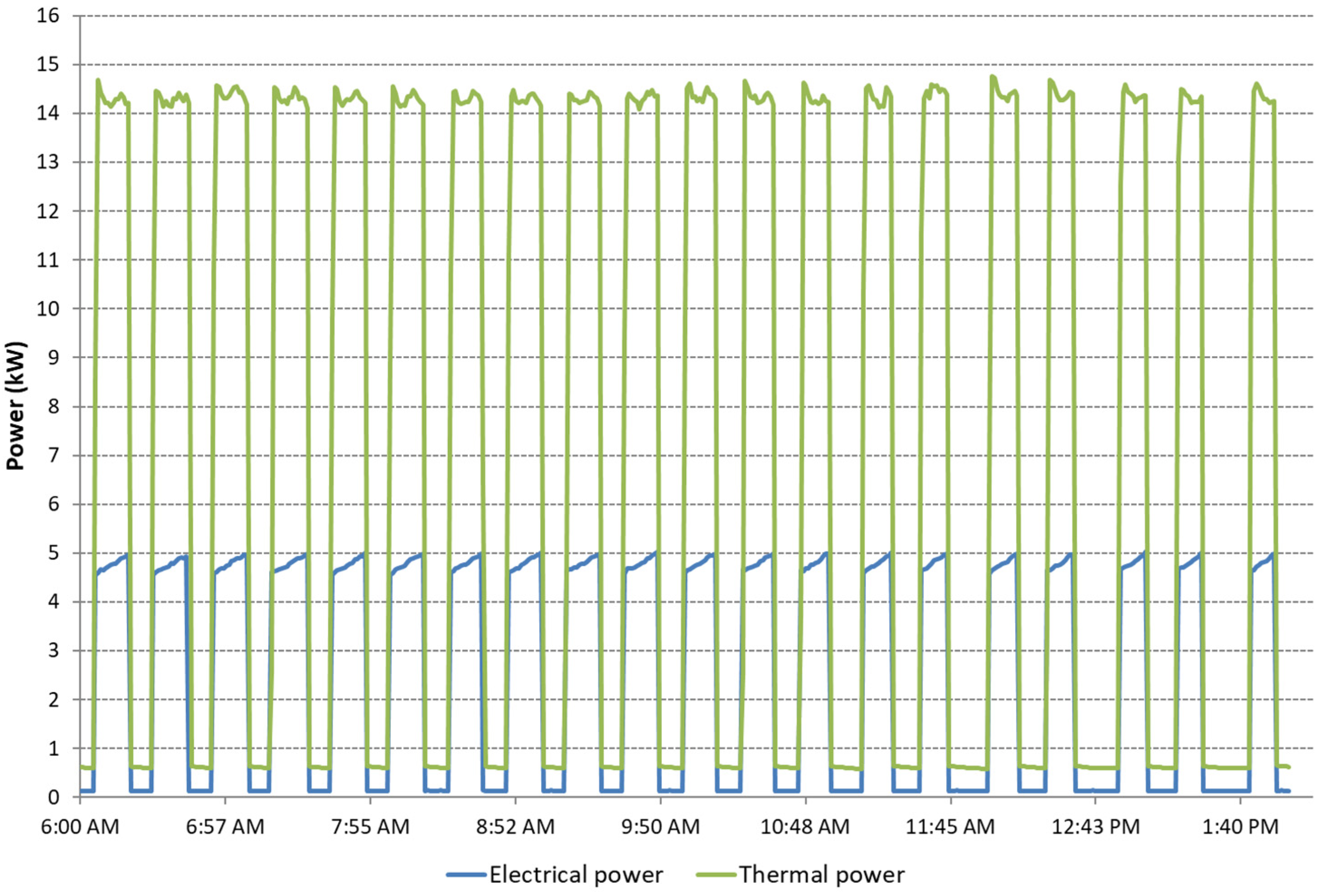
3], where physical, hydrogeological, and energy properties were well-described. A real GSHP system consists of five BHEs (single U-pipe), with a depth of 60 m and buried in a heterogeneous aquifer consisting of alluvial materials (gravel and sandy gravel). The application field of this HVAC system is the air-climatization of a post-weaning piglet room at the Veterinary University of Lodi. Since the ventilation rate requirements are very large, as usually occurs in animal housing, the GSHP system was designed to be an air conditioning system equipped with heat recovery from the exhaust air in order to reduce the energy consumption. The heating and cooling generator was a reversible GSHP (heating capacity 14.4 kW at 40/45 °C on the supply side and 3/0 °C on the ground side; cooling capacity 15.9 kW at 10/15 °C on the supply side and 30/35 °C on the ground side). The warm/cold water produced by the heat pump was stored in a 300 L water tank supplying the heating/cooling coil of an air handling unit (AHU) with a nominal ventilation flow rate of 1200 m3/h. The heat recovery heat exchanger in the AHU had a nominal efficiency equal to 78%. In order to verify the thermo-hygrometric conditions achieved in the piglet room and to measure the energy performance of the GSHP system, a monitoring system was installed to measure the water temperature and flow rate at the heat pump inlet/outlet on the ground and supply sides; the air temperature and relative humidity in several points of the AHU unit and in the piglet room; the air flow rate in the AHU and power consumption by the heat pump; and the AHU. The GSHP system was turned on for a heating period lasting 1 month and the monitoring data were published in [3].
Therefore, to correctly set Type285 in TRNSYS 18, some parameters were retrieved from Alberti et al [3] and others were obtained through the enhanced thermal response test discussed in Antelmi’s study [37]. The complete set of Type285 input data is presented in Appendix B (Table A4 and Table A5).
To exploit the potentiality of Type285, four BHEs (75 m depth) in a square configuration (2 × 2) with a mutual distance of 6 m were implemented. The exchange length meters were equal to the data field, but the number of BHEs was different because this type works better with a square configuration, as discussed below. The unperturbed aquifer temperature was set to be equal to 16.5 °C, coherent with the Lodi shallow aquifer in the autumn period. A Darcy groundwater flow velocity was set to be equal to 1.6∙10−6 m/s according to the interpreted value through the TRT analysis [37].
A uniform thermal conductivity of 3.4 W/m K was assigned to the subsoil domain; this is an equivalent value evaluated for different layers of subsoil consisting of gravel, sand, and clay. This value, correctly inside the thermal conductivity interval defined by the literature for these lithologies, was achieved by sensitivity analyses.
Because of this particular operation of the GSHP system, the mass flow rate and inlet fluid temperature values were also assigned as equal to the experimental data discussed in [3]: the heat pump alternates periods in which the mass flow rate is equal to 0 kg/h to periods with a mass flow rate of 2700 kg/h. The inlet fluid temperature varies according to the heating periods and were enclosed between 5.8 and 17.3 °C.

3. Results

Starting from the physical and hydrogeological conditions discussed above, different numerical simulations in MODFLOW/MT3DMS and TRNSYS were executed and the results are discussed below.

3.1. One BHE Modeling: Comparison between TRNSYS (Type280 and Type557) and MODFLOW/MT3DMS Models for Null Groundwater Flow Velocity

The numerical model implemented in TRNSYS using Type280 (TRNSYS 16) or Type557 (TRNSYS 18) allows for many output variables to be studied, but our attention focused on the exchanged energy by the BHE with the subsoil. The simulated time was 1 year of a conventional GSHP system operation, as discussed above.
In this case, the comparison between the TRNSYS and MODFLOW/MT3DMS models can only be one, because Type557 can only simulate the BHE behavior assuming a zero groundwater flow velocity. Indeed, this type neglects all the advection influences carried out by the BHE on the heat transfer in the aquifer. Implementing the same properties and the same GSHP system operation discussed in the previous paragraphs, a comparison between the two types in terms of the heat rate exchanged by the BHE in the aquifer can be shown in Figure 5 and in Table 5.
The heat rate shown in Figure 5 is calculated by the formula
Q = m ˙ · c p · ( T i n T o u t )
where Q is the heat rate exchanged (W); m is the mass flow rate (kg/h); cp is the specific heat of the fluid (water in this case) (kJ/kg K); Tin and Tout are the inlet/outlet fluid temperature at the top of the U-shape pipe of BHE (°C). The time integral subtended by the heat rate output curves (shown in Figure 5) over time reproduced the energy exchanged by the BHE through the aquifer, and the results are reported in Table 5.
The results (Figure 5 and in Table 5) show that for the null groundwater flow velocity case, the use of Type280 or Type557 was equivalent. The two types exchanged the same amount of energy for each period and both differed from the MODFLOW results of a quantity between 12.6 and 14.4%.

3.2. One BHE Modeling: Comparison between TRNSYS (Type285) and MODFLOW/MT3DMS Models Varying Groundwater Flow Velocity

The new written Type285 implemented in TRNSYS version 18 allowed for the simulation of different groundwater flows and a comparison of the results with the MODFLOW/MT3DMS simulations discussed in [25]. For the sake of simplicity, only the exchanged energy between the BHE and aquifer is shown in Figure 6.
From the exchanged heat rate, according to Equation (6), the extracted or injected energy from the subsoil can be evaluated, as shown in Table 6.
Comparing the differences between the TRNSYS and MODFLOW/MT3DMS results, an average difference of 10% for the heating operation and 6% for the cooling period was carried out. The percentage difference shows good results if compared with the case discussed in [40,41]. For each groundwater flow velocity, starting from the null case, TRNSYS constantly underestimated the exchanged energy computed in MODFLOW models; the difference was approximately constant for the heating/cooling period, and was equal to −11% and −13% for the null Darcy velocity and −14% and −5% for the Darcy velocity equal to 5 ∙ 10−6 m/s, respectively. The maximum groundwater velocity case showed a greater difference between the two software programs and equal to −20% (heating) and −12% (cooling) because the advection term became predominant over the diffusion thermal term. This result is justified because logarithmic approximation is less effective for higher groundwater flow velocities. The global differences are acceptable because they were lower than 15%. Therefore, the use of the new Type285 in TRNSYS 18 is suggested for one BHE modeling where the groundwater flow velocities are not null. In general, as discussed in [25], this approach confirms that the exchanged energy increases when the groundwater flow velocity increases; the percentage of increase related to the null groundwater flow case is shown in Table 7.
Table 7 demonstrates the energy performance increase in the BHE due to the increasing groundwater flow velocity. Specifically, for the maximum groundwater flow velocity case, for the heating period, an increase of 81% was achieved in TRNSYS (101% in MODFLOW model) and for the cooling period, an increase of 81% was achieved in TRNSYS (79% in MODFLOW model). These results are also in accordance with other studies in the literature [9,10,38].
This difference was also detectable in the aquifer temperature values for different monitoring points located downgradient of the BHE. For instance, at any given time during the simulation (here reported as the last day of the heating and cooling period), the aquifer temperature variation can be shown for the minimum Darcy velocity (Figure 7a) and for the maximum velocity (Figure 7b).
The ground temperature again showed a certain difference between TRNSYS and MODFLOW. The absolute residual mean difference between the ground temperature achieved in TRNSYS and in MODFLOW for the null velocity was equal to 0.52 °C (heating) and 0.70 °C (cooling), whereas the 10−5 m/s flow velocity case was equal to 0.42 °C (heating) and 0.63 °C (cooling). A conventional value of the temperature difference between the heat carrier fluid of the BHE and the ground can be assumed to be equal to 5 °C, so the maximum absolute mean difference was 0.7 °C. Therefore, the same difference of approximately 13% between the two models was found.

3.3. Bore Field Modeling: Sensitivity Analyses

By means of Type285, the definition of a number of BHEs greater than one in the homogeneous aquifer is possible by modifying the parameters “Nb” (number of BHE) and “Vst” (the storage volume). Many configurations can be implemented, but the best one is square geometry, reproducing a regular bore field with a square layout (i.e., 2 × 2, 3 × 3, 4 × 4, etc.). When the user introduces a number of BHEs greater than one, the storage radius defined in Equation (4) is not the radius of the temperature perturbation, but represents the mutual distance between the BHE. In this case, Equation (6) can be rewritten as follows:
V s t o r a g e = N b · d x · d y · H
where dx and dy are the mutual distances between BHE along the X and Y direction (m) and H is the BHE depth (m). The simulations were carried out considering nine BHE in the domain with a single U-shape pipe, connected in parallel with a mass flow rate equal to 1000 kg/h; the mutual distance between BHE was varied and equal to 2, 5, 8, and 15 m. The remaining physical and hydrogeological properties were the same as discussed above. The exchanged heat rate is shown in Figure 8, while the exchanged energy is shown in Table 8.
The results show that exchanged energy increases when the mutual distance between the BHE increases. This is correct, because the higher the distance between BHE, the lower the thermal interference between adjacent BHE; therefore, the energy performance of the GSHP system improves when the BHEs are located at the correct position without interferences between each other. For this specific null flow velocity case, the correct distance between BHE was greater than 8 m, because the thermal plume was radial and not developed along the flow direction [32,33]. When different BHE are installed in hydrogeological settings with high flow velocities, the distance could be reduced because of the different shape of the thermal plume. Indeed, considering the maximum storage volume simulated, the exchanged heat rate seemed to be at the steady-state condition at the end of both the heating and cooling operations.

3.4. Bore Field Modeling: Validation of the Type 285 with Real Experimental Data

To validate the numerical modeling of a bore field using Type285, a set of experimental data was compared with the simulated ones. A monitoring campaign of the geothermal system discussed in Section 2.5 was carried out for a month in 2016, namely from 26 October to 25 November. During that period, 50 piglets were hosted in the post-weaning room. The request from the veterinary research team for this special experimentation was for it to maintain at approximately 28–30 °C for the experimental period inside the room. The heat pump switched off whenever the water temperature at the storage tank outlet rose above the set point, equal to 48.5 °C, then the electrical power fell to zero. When the heat pump was turned on, the absorbed electrical power was in the range of 4.6–4.9 kW and the thermal power absorbed by the subsoil was about 14–15 kW. Depending on the day of the experimental period, the values could vary slightly according to the variation in the external weather condition. A typical daily operation of the heat pump is reported Figure 9.
Assuming the values reported in Appendix B, the numerical simulation implementing Type285 was run in TRNSYS 18. This time, the simulation length was equal to 1 month like the experimental data; the output results of the exchanged power are reported for just one representative week (from 10 to 17 November) of the month, as shown in Figure 10.
The experimental and simulated exchanged power values were reported for every minute, so for the sake of simplicity, only one representative week was reported in the figure. The heat pump was not equipped with an inverter, hence it alternated between on and off cycles to maintain the temperature at 28–30 °C inside the piglet room. Because of this operation, the null exchanged power values are representative of situations where the heat pump is turned off; values between 0 and 13 kW are representative of a dynamic state when the heat pump is turning on or off; and values between 13 and 15 kW are representative of the steady condition when the heat pump is turned on and is running at full power. The comparison between the experimental and simulated data is reported in Table 9.
The comparison between the experimental and simulated heat rates was not easily readable because the values were taken with a small time interval, so it was difficult to have a clear situation of the comparison. The values of the exchanged powers can be seen in the table: the experimental values agreed with the simulated ones, but the comparison was less significant because it was punctual for every minute. A better comparison can be achieved by looking at the values of the total exchanged energy for the experimental period: specifically, the simulated exchanged energy value was equal to 4254.2 kWh, corresponding to an underestimation of 8.5% than that in the experimental data, which was equal to 4667 kWh. Therefore, it is possible to conclude that Type285 is adequate for simulating the BHE and bore field, considering all the phenomena that usually happen for heat transport in aquifer (from conduction to advection processes).

4. Discussion

The results of the simulations can be summarized as follows:
Concerning the numerical simulations of one BHE, the advantages of the approach by means of TRNSYS software are:
  • For one BHE modeling, identical hydrogeological property conditions and null flow velocity, the results of Type280 are equal to the results of Type557.
  • For one BHE modeling, identical hydrogeological properties and null flow velocity, the results of Type285 were in accordance with the results in the general literature and specific numerical MODFLOW/MT3DMS model: the exchanged energies differed with a quantity lower than 13% and the ground temperature differences were lower than 0.7 °C;
  • For one BHE modeling, identical hydrogeological properties and different groundwater flow velocities, the Type285 model results agreed with the MODFLOW/MT3DMS results: on average, the exchanged energy differed by less than 11.6% and the ground temperature difference was lower than 0.6 °C.
Concerning the numerical simulations with one BHE, the limitations were as follows:
  • Type280 is only available for TRNSYS 16;
  • Type557 can only simulate the conduction processes (null groundwater flow case);
  • The definition of many parameters in Type280, Type557, and Type285;
  • Simplified approach with radial geometry for the groundwater flow in the DST model.
Concerning the numerical simulations of the bore field, the advantages areas follows:
  • It is useful for configurations of a bore field with a square mesh layout (i.e., 2 × 2, 3 × 3, 4 × 4, etc.);
  • Good results for the synthetic case with nine BHEs and null flow velocity: as the distance between BHE increased (range of 2–15 m), the energy exchanged by the HVAC system increased by 41% and the thermal plume in the subsoil was less extensive (less overlap effects);
  • Through the possibility of implementing different BHE (bore field) in a single model, the numerical simulation of borehole thermal energy storage (BTES) is possible, assuming different hydrogeological conditions.
Concerning the numerical simulations of the bore field, the limits are as follows:
  • Because of the radial geometry (DST physical model), the simulation of the BHE configuration fit the square geometry layout well, but was limited for the remaining layout as well as for flow velocities greater than 0 m/d, and the problems around the bore field increase for higher velocities.

5. Conclusions

The aim of this study was to create a new numerical element in TRNSYS, which is a non-standard type (named Type285 for TRNSYS 18) that users can exploit to improve the HVAC system design. Specifically, this type is a helpful tool for the numerical simulation of one or more BHE, consisting of one or double U-shape pipes buried in a homogeneous or heterogeneous aquifer, where a heat carrier fluid circulates and exchanges heat with the surrounding subsoil (closed loop system). Through the new type, the simulation of the BHE energy performance assuming different hydrogeological conditions (i.e., variations of the Darcy groundwater flow velocity) is now possible. This issue is of great importance because the increase in the groundwater flow velocity due to the geology of the site can lead to an increase in the BHE energy performance up to 100%, as demonstrated in the literature [9,10,25,34,35]. Up to now, this issue has been well-discussed by hydrogeological code (i.e., MODLOW, FEFLOW, etc.) and it is also now possible to take this into account in the software mainly used for energy purposes. The need to reproduce BHE simulations using the correct approach was essential in the development of the Fusion Grant project, a research project shared between Inewa s.r.l. and EURAC Research on the topic of the DSHP system. In the Fusion Grant project, different tests were carried out on a DSHP in the laboratory and the role of the numerical model of the BHE coupled to a heat pump was essential to target the test. Therefore, coupling the experimental test and numerical simulations will allow us to improve the energy efficiency of the DSHP system.
The code of Type285 was developed starting from Type280 and Type557, written on the basis of the TRNVDSTP model [39]. As a first result, for identical aquifer properties, a comparison between Type280 and Type557 was carried out: the results were in accordance only for the null groundwater flow velocity because Type557 could not implement advection terms related to the groundwater flow velocity. Type285 was then written and compiled by assuming a logarithmic approach between the exchanged energy between the BHE and ground and the Darcy flow velocity increase, as the MODFLOW/MT3DMS models suggest. A comparison between TRNSYS and MODFLOW/MT3DMS has already been made, but showed differences between the two approaches. The creation of Type285 overcame this difference and showed a good agreement between TRNSYS 18 and MODFLOW/MT3DMS: specifically, assuming the hydrogeological and physical properties of the synthetic model created in MODFLOW/MT3DMS [25], the exchanged energy between BHE and the aquifer in TRNSYS and MODFLOW/MT3DMS was lower than an average quantity of 11.6% for any hydrogeological setting. This also confirms that TRNSYS 18, using the Type285, is now able to reproduce the numerical modeling of one BHE in a heterogenous aquifer with an acceptable approximation.
Furthermore, in the TRNSYS 18 model, a sensitivity analysis on the mutual distances between BHE was carried out and correctly showed that the higher the distance, the lower the thermal interference between BHE, and the greater the energy performance of the system. This step is in preparation to the final validation of Type285 in accordance with the experimental data of a real GSHP system installed in Lodi. The exchanged energy between the BHE and ground estimated by the GSHP system, through a special monitoring system, was equal to 4667 kWh [3], whereas the simulated energy by the model was equal to 4254.2 kWh, corresponding to an underestimation of about 8.5%. Even in this case, the TRNSYS model agreed with the experimental results with an acceptable approximation.
Therefore, Type285 can now be easily implemented in TRNSYS 18 and provides the possibility to reproduce one or more than one BHE in a homogeneous or heterogeneous aquifer such as hydrogeological software. Furthermore, this approach could be a helpful tool for scientists and technicians to provide preliminary analyses concerning the sizing of the bore field in the design of GSHP or DSHP systems.

Author Contributions

Conceptualization, R.F., M.A. and A.Z.; Methodology, M.A., R.F. and F.T.; Software, M.A. and F.T.; Validation, M.A. and F.T.; Investigation, M.A.; Resources, R.F. and A.Z; data curation, M.A.; Writing—original draft preparation, M.A.; Writing—review and editing, M.A., A.Z., F.T. and R.F.; Visualization, M.A.; Supervision, A.Z. and R.F.; Funding acquisition, R.F. All authors have read and agreed to the published version of the manuscript.

Funding

This research received no external funding.

Data Availability Statement

Not applicable.

Acknowledgments

The authors thank D. Pahud for sharing the last version of the TRNVDSTP code and for providing suggestions about the code.

Conflicts of Interest

The authors declare no conflict of interest.

Appendix A

Here is a list of the parameters, input, and output set into Type285 for the synthetic case.
Table A1. Parameters implemented into Type285.
ParameterDescriptionValueUnit
VStorage volume64,884.9m3
HBorehole depth100m
DPHHeader depth0m
NbNumber of boreholes1-
roBorehole radius0.14m
NSerieNumber of boreholes in series1-
NRLocNumber of radial regions1-
NZLocNumber of vertical regions1-
ksStorage thermal conductivity8.24kJ/h m K
CsStorage heat capacity752.73kJ/m3 K
RpNegative of U-tubes/bore−1-
RpoOuter radius of U-tube pipe0.0237M
RpiInner radius of U-tube pipe0.02M
dCenter-to-center half distance0.03M
λbhFill thermal conductivity8.24kJ/h m K
λpPipe thermal conductivity1.38kJ/h m K
λGAPGap thermal conductivity1kJ/h m K
GAPGap thickness0M
VrefReference borehole flowrate1000Kg/h
TrefReference temperature20°C
RaPipe-to-pipe heat transfer−1-
cfFluid specific heat4.186kJ/h kg K
rfFluid density999Kg/m3
ISOInsulation indicator0-
FRISOInsulation height fraction0-
THinsInsulation thickness0M
kinsInsulation thermal conductivity1kJ/h m K
SYNumber of simulation years1Y
TmaxMaximum storage temperature50°C
TgsInitial surface temperature of storage volume11.81°C
DTGInitial thermal gradient of storage volume0K/m
IPRENumber of preheating years0-
φPreheat phase delay0D
TmaAverage air temperature—Preheat years0°C
TaaAmplitude of air temperature—Preheat years0°C
φairAir temperature phase delay—Preheat years0D
NlNumber of ground layers1-
kgThermal conductivity of the layer8.24kJ/h m K
cgHeat capacity of the layer752.73kJ/m3 K
THgThickness of the layer150m
-Not used (Printing 1)--
-Not used (Printing 2)--
VdDarcy groundwater velocity0.00001m/s
KDAR1Constant value 1 that multiplies the ln (Vd)0.1889-
KDAR2Constant value 21.83412-
The Vref parameter is only used to evaluate the thermal resistance from BHE to the ground and is not used to reproduce the real circulating flow rate. The heat carrier flow rate value needs to be implemented into the “m” parameter defined in the input section.
If −11 ≤ Rp ≤ 0, the calculation of the thermal resistance between the heat carrier fluid and the ground surrounding the BHE is specified, and the value can be found in the DST.DAT file (if IPRT = 1). The default value suggested is −1.
The KDAR1 and KDAR2 values can be modified if the users approximate the exchanged energy values and the multiplying factor with a different approach technique.
Table A2. Input implemented into Type285.
ParameterDescriptionValueUnit
TinInlet fluid temperature1 or 28 *°C
m’Inlet flowrate (Total)1000 **Kg/h
TairhTemperature on top of storage11.81 ***°C
TairAir temperature11.81 ***°C
CirculCirculation switch1-
* The inlet fluid temperature into the U-shape pipe was set as constant and equal to 1 °C in the heating period (from 0 to 183 d) and 28 °C in the cooling period (from 243 d to 336 d). In the remaining periods (spring and autumn periods), an inlet fluid temperature of 0 °C was set, but was not read because the related mass flow rate was null. ** The mass flow rate of the BHE was time dependent as the inlet fluid temperature was equal to 1000 kg/h when the GSHP system was turned on and equal to 0 kg/h when the GWHP system was turned off. A summary of the GSHP system operation is shown in Table 3. *** The yearly mean air temperature of Milano city was implemented for both air temperature on top of the storage and elsewhere on the storage volume. The value was derived by linking Type285 to a climatic file of Milano city, where the yearly mean air temperature is constant and equal to 11.81 °C.
Table A3. Output implemented into Type285.
ParameterDescriptionValueUnit
ToutOutlet temperature-°C
m’Outlet flowrate (Total)-Kg/h
Tav.stAverage storage temperature-°C
Q’Average heat transfer rate-kJ/h
Qloss, tHeat loss through top of storage-kJ/h
Qloss, sHeat loss through side of storage-kJ/h
Qloss, bHeat loss through bottom of storage-kJ/h
QDSTInternal energy variation-kJ/h
Tav.bhAverage soil temperature near boreholes-°C
Tbh,1Average soil temperature near boreholes: center-°C
Tbh,2Average soil temperature near boreholes: edges-°C
ToutOutlet temperature-°C
m’Outlet flowrate (Total)-Kg/h

Appendix B

Here a list of the parameters, input, and output set into Type285 for the field case.
Table A4. Parameters implemented into Type285.
ParameterDescriptionValueUnit
VStorage volume64,884.9m3
HBorehole depth100M
DPHHeader depth0M
NbNumber of boreholes1-
roBorehole radius0.14M
NSerieNumber of boreholes in series1-
NRLocNumber of radial regions1-
NZLocNumber of vertical regions1-
ksStorage thermal conductivity8.24kJ/h m K
CsStorage heat capacity752.73kJ/m3K
RpNegative of U-tubes/bore−1-
RpoOuter radius of U-tube pipe0.0237M
RpiInner radius of U-tube pipe0.02M
dCenter-to-center half distance0.03M
λbhFill thermal conductivity8.24kJ/h m K
λpPipe thermal conductivity1.38kJ/h m K
λGAPGap thermal conductivity1kJ/h m K
GAPGap thickness0m
VrefReference borehole flowrate1000Kg/h
TrefReference temperature20°C
RaPipe-to-pipe heat transfer-1-
cfFluid specific heat4.186kJ/h kg K
rfFluid density999Kg/m3
ISOInsulation indicator0-
FRISOInsulation height fraction0-
THinsInsulation thickness0M
kinsInsulation thermal conductivity1kJ/h m K
SYNumber of simulation years1Y
TmaxMaximum storage temperature50°C
TgsInitial surface temperature of storage volume11.81°C
DTGInitial thermal gradient of storage volume0K/m
IPRENumber of preheating years0-
φPreheat phase delay0D
TmaAverage air temperature—Preheat years0°C
TaaAmplitude of air temperature—Preheat years0°C
φairAir temperature phase delay—Preheat years0D
NlNumber of ground layers1-
kgThermal conductivity of layer8.24kJ/h m K
cgHeat capacity of layer752.73kJ/m3 K
THgThickness of layer150m
-Not used (Printing 1)--
-Not used (Printing 2)--
VdDarcy groundwater velocity0.00001m/s
KDAR1Constant value 1 that multiplies the ln (Vd)0.1889-
KDAR2Constant value 21.83412-
The Vref parameter is only used to evaluate the thermal resistance from BHE to the ground and is not used to reproduce the real circulating flow rate. The heat carrier flow rate value needs to be implemented into the “m” parameter defined in the input section.
If −11 ≤ Rp ≤ 0, the calculation of the thermal resistance between the heat carrier fluid and the ground surrounding the BHE is specified and the value can be found in the DST.DAT file (if IPRT = 1). The default value suggested is −1.
The KDAR1 and KDAR2 values can be modified if the users approximate the exchanged energy values and the multiplying factor with a different approach technique.
Table A5. Input implemented into Type285.
ParameterDescriptionValueUnit
TinInlet fluid temperature1 or 28 *°C
m’Inlet Flowrate (Total)1000 **Kg/h
TairhTemperature on Top of Storage11.81 ***°C
TairAir Temperature11.81 ***°C
CirculCirculation Switch1-
* The inlet fluid temperature into the U-shape pipe was set as constant and equal to 1 °C at the heating period (from 0 to 183 d) and 28 °C at the cooling period (from 243 d to 336 d). In the remaining periods (spring and autumn periods), an inlet fluid temperature of 0 °C was set but not read because the related mass flow rate was null. ** The mass flow rate of the BHE was time dependent as the inlet fluid temperature, and was equal to 1000 kg/h when the GSHP system was turned on and equal to 0 kg/h when the GWHP system was turned off. A summary of the GSHP system operation in Table 3. *** The yearly mean air temperature of Milano city was implemented for both the air temperature on top of the storage and elsewhere on the storage volume. The value was derived linking Type285 to a climatic file of Milano city, where the yearly mean air temperature is constant and equal to 11.81 °C.

References

  1. Piga, B.; Casasso, A.; Pace, F.; Godio, A.; Sethi, R. Thermal impact assessment of groundwater heat pumps (GWHPs): Rigorous vs. simplified models. Energies 2017, 10, 1385. [Google Scholar] [CrossRef] [Green Version]
  2. Farabi-asl, H.; Chapman, A.; Itaoka, K.; Noorollahi, Y. Ground source heat pump status and supportive energy policies in Japan. Energy Procedia 2019, 158, 3614–3619. [Google Scholar] [CrossRef]
  3. Alberti, L.; Antelmi, M.; Angelotti, A.; Formentin, G. Geothermal heat pumps for sustainable farm climatization and field irrigation. Agric. Water Manag. 2018, 195, 187–200. [Google Scholar] [CrossRef]
  4. Torres Sevilla, L.; Radulovic, J. Effectiveness of Thermal Properties in Thermal Energy Storage Modeling. Front. Mech. Eng. 2021, 7, 1–13. [Google Scholar] [CrossRef]
  5. Hemmerle, H.; Ferguson, G.; Blum, P.; Bayer, P. The evolution of the geothermal potential of a subsurface urban heat island. Environ. Res. Lett. 2022, 17, 084018. [Google Scholar] [CrossRef]
  6. Bayer, P.; Saner, D.; Bolay, S.; Rybach, L.; Blum, P. Greenhouse gas emission savings of ground source heat pump systems in Europe: A review. Renew. Sustain. Energy Rev. 2020, 16, 1256–1267. [Google Scholar] [CrossRef]
  7. Basta, S.; Minchio, F. Geotermia e Pompe di Calore. Guida Pratica agli Impianti Geotermici di Climatizzazione; Villaggio Globale: Rome, Italy, 2007; pp. 1–439. ISBN 978-88-903170-0-2. [Google Scholar]
  8. Diao, N.; Li, Q.; Fang, Z. Heat transfer in ground heat exchangers with groundwater advection. Int. J. Therm. Sci. 2004, 43, 1203–1211. [Google Scholar] [CrossRef]
  9. Fujii, H.; Itoi, R.; Fujii, J.; Uchida, Y. Optimizing the design of large-scale ground-coupled heat pump systems using groundwater and heat transport modeling. Geothermics 2005, 34, 347–364. [Google Scholar] [CrossRef]
  10. Fan, R.; Jiang, Y.; Yao, Y.; Shiming, D.; Ma, Z. A study on the performance of a geothermal heat exchanger under coupled heat conduction and groundwater advection. Energy 2007, 32, 2199–2209. [Google Scholar] [CrossRef]
  11. Molina-Giraldo, N.; Blum, P.; Zhu, K.; Bayer, P.; Fang, Z. A moving finite line source model to simulate borehole heat exchangers with groundwater advection. Int. J. Therm. Sci. 2011, 50, 2506–2513. [Google Scholar] [CrossRef]
  12. Pasquier, P.; Lamarche, L. Analytic Expressions for the Moving Infinite Line Source Model. SSRN Electron. J. 2022, 103, 102413. [Google Scholar] [CrossRef]
  13. Belliardi, M.; Cereghetti, N.; Caputo, P.; Ferrari, S. A method to analyze the performance of geocooling systems with borehole heat exchangers. Results in a monitored residential building in southern alps. Energies 2021, 14, 7407. [Google Scholar] [CrossRef]
  14. Hellstrom, G. Ground Heat Storage. Thermal Analyses of Duct Storage Systems. Ph.D. Thesis, University of Lund, Lund, Sweden, 1996. [Google Scholar]
  15. Klein, S.A.; Beckman, W.A. TRNSYS 16 Manual; University of Wisconsin-Madison: Madison, WI, USA, 2004; Volume 1. [Google Scholar]
  16. Thorén, A. Practical Evaluation of Borehole Heat Exchanger Models in TRNSYS; KTH School of Industrial Engineering and Management Energy Technology: Stockholm, Sweden, 2016. [Google Scholar]
  17. De Rosa, M.; Ruiz-calvo, F.; Corberán, J.M.; Montagud, C.; Tagliafico, L.A. A novel TRNSYS type for short-term borehole heat exchanger simulation: B2G model. Energy Convers. Manag. 2015, 100, 347–357. [Google Scholar] [CrossRef] [Green Version]
  18. De Rosa, M.; Ruiz-Calvo, F.; Corberàn, J.M.; Montagud, C.; Tagliafico, L.A. Borehole modelling: A comparison between a steady-state model and a novel dynamic model in a real ON/OFF GSHP operation. J. Phys. Conf. Ser. 2014, 547, 012008. [Google Scholar] [CrossRef] [Green Version]
  19. Cazorla-marín, A.; Montagud-montalvá, C.; Tinti, F.; Miguel, J.; Universitario, I.; De Ingeniería, D.I.; Iuiie, E.; De València, U.P. A novel TRNSYS type of a coaxial borehole heat exchanger for both short and mid term simulations: B2G model. Appl. Therm. Eng. 2020, 164, 114500. [Google Scholar] [CrossRef]
  20. Huber, A. Software Manual Program EWS Calculation of Borehole Heat Exchangers; Hube Energietechnik: Zurich, Switzerland, 2008. [Google Scholar]
  21. BLOCON EED on the Web-Earth Energy Designer for Power Users; BLOCON: Lund, Sweden, 2018.
  22. Xu, X.; Spitler, J. Modeling of Vertical Ground Loop Heat Exchangers with Variable Convective Resistance and Thermal Mass of the Fluid. Methodology 2005, 8, 1. [Google Scholar]
  23. Pahud, D.; Fromentin, A. PILESIM: A simulation tool for pile and borehole heat exchanger systems. Bull. Hydrogblogie 1999, 17, 323–330. [Google Scholar]
  24. Xu, L.; Guo, F.; Hoes, P.J.; Yang, X.; Hensen, J.L.M. Investigating energy performance of large-scale seasonal storage in the district heating system of chifeng city: Measurements and model-based analysis of operation strategies. Energy Build. 2021, 247, 111113. [Google Scholar] [CrossRef]
  25. Angelotti, A.; Alberti, L.; La Licata, I.; Antelmi, M. Energy performance and thermal impact of a Borehole Heat Exchanger in a sandy aquifer: Influence of the groundwater velocity. Energy Convers. Manag. 2014, 77, 700–708. [Google Scholar] [CrossRef]
  26. Diersch, H.J.G.; Bauer, D.; Heidemann, W.; Rühaak, W.; Schätzl, P. FEFLOW 6.1-Finite Element Subsurface Flow & Transport Simulation System. DHI-Wasy Softw. User Man. 2010, 104, 1. [Google Scholar]
  27. Casasso, A.; Sethi, R. Efficiency of closed loop geothermal heat pumps: A sensitivity analysis. Renew. Energy 2014, 62, 737–746. [Google Scholar] [CrossRef] [Green Version]
  28. Diersch, H.-J.G.; Rühaak, W.; Schätzl, P.; Renz, A. A new method for modelling geothermal heat exchangers in shallow aquifer systems. In Proceedings of the Numerische Grund-Wasser-Modellierung Konzeption, komplexe Anwendung, Entscheidungsgrundlage, Graz, Austria, 24–25 June 2008; pp. 20–23. [Google Scholar]
  29. Zheng, C.; Wang, P.P. MT3DMS: A Modular Three-Dimensional Multispecies Transport Model for simulation of advection, dispersion and chemical reactions of contaminants in groundwater systems. Contract Rep. 1999, 239, 1. [Google Scholar]
  30. Panday, S.; Langevin, C.D.; Niswonger, R.G.; Ibaraki, M.; Hughes, J.D. MODFLOW–USG Version 1: An Unstructured Grid Version of MODFLOW for Simulating Groundwater Flow and Tightly Coupled Processes Using a Control Volume Finite-Difference Formulation. Geol. Surv. 2013, 66, 1. [Google Scholar]
  31. Panday, S. USG-Transport Version 1.5.0: The Block-Centered Transport (BCT) Process for MODFLOW-USG; GSI Environment: Irvine, CA, USA, 2020. [Google Scholar]
  32. Antelmi, M.; Alberti, L.; Barbieri, S.; Panday, S. Simulation of thermal perturbation in groundwater caused by Borehole Heat Exchangers using an adapted CLN package of MODFLOW-USG. J. Hydrol. 2021, 596, 126106. [Google Scholar] [CrossRef]
  33. Barbieri, S.; Antelmi, M.; Panday, S.; Baratto, M.; Angelotti, A.; Alberti, L. Innovative numerical procedure for simulating borehole heat exchangers operation and interpreting thermal response test through MODFLOW-USG code. J. Hydrol. 2022, 614, 128556. [Google Scholar] [CrossRef]
  34. Chiasson, A.D.; Rees, S.J.; Spitler, J.D. Preliminary assessment of the effects of groundwater flow on closed-loop ground-source heat pump systems. ASHRAE Trans. 2000, 106, 380–393. [Google Scholar]
  35. Alberti, L.; Angelotti, A.; Antelmi, M.; La Licata, I. Borehole Heat Exchangers in aquifers: Simulation of the grout material impact. In Rendiconti Online Societa Geologica Italiana; Rendiconti: Rome, Italy, 2016; pp. 28–271. [Google Scholar] [CrossRef]
  36. Hecht-Méndez, J.; Molina-Giraldo, N.; Blum, P.; Bayer, P. Evaluating MT3DMS for heat transport simulation of closed geothermal systems. Groundwater 2010, 48, 741–756. [Google Scholar] [CrossRef]
  37. Antelmi, M.; Alberti, L.; Angelotti, A.; Curnis, S.; Zille, A.; Colombo, L. Thermal and hydrogeological aquifers characterization by coupling depth-resolved thermal response test with moving line source analysis. Energy Convers. Manag. 2020, 225, 113400. [Google Scholar] [CrossRef]
  38. Wang, H.; Qi, C.; Du, H.; Gu, J. Thermal performance of borehole heat exchanger under groundwater flow: A case study from Baoding. Energy Build. 2009, 41, 1368–1373. [Google Scholar] [CrossRef]
  39. Pahud, D.; Fromentin, A.; Hadorn, J.-C. The Duct Ground Ground Heat Storage Model (DST) for TRNSYS Used for the Simulation of Heat Exchanger Piles; DST: Lausanne, Sweden, 1996. [Google Scholar]
  40. Antelmi, M.; Legrenzi, C. Geotermia a bassa entalpia: Simulazione dello scambio termico in acquiferi mediante i codici Modflow e Trnsys. In VIII Forum Italiano di Scienze della Terra; Politecnico di Milano: Milano, Italy, 2010. [Google Scholar]
  41. Alberti, L.; Angelotti, A.; Antelmi, M.; La Licata, I.; Legrenzi, C. Low temperature geothermal energy: Heat exchange simulation in aquifers through Modflow/MT3DMS codes. AQUA Mundi 2012, 39–51. [Google Scholar] [CrossRef]
  42. Angelotti, A.; Alberti, L.; La Licata, I.; Antelmi, M. Borehole heat exchangers: Heat transfer simulation in the presence of a groundwater flow. J. Phys. Conf. Ser. 2014, 501, 012033. [Google Scholar] [CrossRef] [Green Version]
  43. Alberti, L.; Angelotti, A.; Antelmi, M.; La Licata, I. A numerical study on the impact of grouting material on borehole heat exchangers performance in aquifers. Energies 2017, 10, 703. [Google Scholar] [CrossRef]
Figure 1. DST model: Comparing local and global problems.
Energies 16 01288 g001
Figure 2. Exchanged power for the heating and cooling period evaluated in MODFLOW/MT3DMS (MF2000_v0 and v-5) and TRNSYS (v0 and v-5) for the Darcy velocities equal to 0 and 10−5 m/s.
Energies 16 01288 g002
Figure 3. Exchanged energies for the heating and cooling period evaluated in MODFLOW/MT3DMS by varying the Darcy groundwater flow velocities.
Energies 16 01288 g003
Figure 4. Multiplying factors of the exchanged energies varying the Darcy groundwater flow velocities.
Energies 16 01288 g004
Figure 5. Exchanged heat rate for the TRNSYS (Type280 and Type557) and MODFLOW/MT3DMS simulations for the null groundwater flow velocity.
Energies 16 01288 g005
Figure 6. Exchanged heat rate for the TRNSYS and MODFLOW simulations with varying groundwater flow velocities.
Energies 16 01288 g006
Figure 7. (a) Ground temperature downgradient of the BHE rate for the TRNSYS and MODFLOW simulations at the end of the heating period (183 d) and cooling period (336 d) for the null case velocity. (b) Ground temperature downgradient of the BHE for a groundwater flow velocity equal to 10−5 m/s.
Energies 16 01288 g007
Figure 8. Exchanged heat rate for TRNSYS in the case of nine BHE, null groundwater flow velocity, and increasing mutual distances between BHE: (Vst2) storage volume equal to 3636 m3; (Vst5) 22,725 m3; (Vst8): 58,176 m3; (Vst15): 204,525 m3.
Energies 16 01288 g008
Figure 9. Heat pump operation on a representative day (12 November) of the experimental heating period (from 6 a.m. to 2 p.m.).
Energies 16 01288 g009
Figure 10. Experimental and simulated exchanged power for one representative week of the heating experimental period.
Energies 16 01288 g010
Table 1. Exchanged energy in the heating and cooling periods for the TRNSYS and MODFLOW simulations.
Darcy Flow Velocity (m/s)TRNSYS
(kWh)
% Vd vs. V0 MODFLOW/MT3DMS (kWh)% Vd vs. V0
Vd = 0 m/s (winter)5923.0-6051.6-
Vd = 10−5 m/s (winter)6429.5+9%15,022.4+148%
Vd = 0 m/s (summer)8925.2-8944.3-
Vd = 10−5 m/s (summer)10,161.7+1423,463.4+162%
Table 2. Multiplying factors for the exchanged energy between the BHE and ground.
Darcy Flow Velocity (m/d)Multiplying Factor (-)
0.008641.00
0.08641.24
0.4321.69
0.8641.86
Table 3. The BHE and hydrogeological properties.
ParameterValueUnit
Storage volume64,884.9m3
Number of BHE1-
BHE length100m
Outer radius of drilling0.14m
Thermal conductivity of the storage and grout material8.24kJ/h m K
Volumetric heat capacity of the storage material752.7kJ/m3 K
Outer radius of the U-shape pipe0.0237m
Inner radius of the U-shape pipe0.02m
Thermal conductivity of the pipe material1.4kJ/h m K
Reference fluid flow rate per BHE1000kg/h
Initial temperature of the undisturbed ground surface11.8°C
Thermal conductivity of the aquifer8.24kJ/h m K
Volumetric heat capacity of the aquifer752.7kJ/m3 K
Darcy groundwater flow velocity0 ÷ 10−5m/s
Table 4. Yearly operation conditions of the BHE system.
OperationTime Length (d)Inlet Temperature to the BHE (°C)
Heating (ON)1831
Pause (OFF)60-
Cooling (ON)9328
Pause (OFF)29-
Table 5. Exchanged energy in the heating and cooling periods for TRNSYS simulations with null flow velocity.
Darcy Velocity (m/s)Eheating (kWh)Ecooling (kWh)
Type280 Type557 MODFLOW Type280 Type557 MODFLOW
010,54610,54611,8728858885810,141
Table 6. Exchanged energy in the heating and cooling periods for the TRNSYS and MODFLOW simulations.
Darcy Velocity (m/s)Eheating (kWh)DifferenceEcooling (kWh)Difference
TRNSYS MODFLOW TRNSYS MODFLOW
010,54611,872−11%885810,141−13%
10−710,54611,982−12%885810,114−12%
10−614,46514,667−1%12,14911,2688%
5 × 10−617,67120,572−14%14,84215,671−5%
10−519,05223,889−20%16,00218,189−12%
Table 7. Increase percentage in the exchanged energy against the null groundwater flow case for the TRNSYS and MODFLOW simulations.
Darcy Velocity (m/s)Heating—% Vd vs. Vd0Cooling—% Vd vs. Vd0
TRNSYSMODFLOWTRNSYSMODFLOW
0----
10−70%1%0%0%
10−637%24%37%11%
5 × 10−668%73%68%55%
10−581%101%81%79%
Table 8. Exchanged energy in the heating and cooling periods for the TRNSYS simulations.
Storage Volume (m3)Eheating (kWh)DifferenceEcooling (kWh)Difference
363623,904-21,941-
22,72530,45127%27,16924%
58,17632,61536%27,72626%
204,52533,71541%27,07723%
Table 9. Exchanged power and energy for the experimental or simulated data.
Q min (kW)Q max (kW)Q mean (kW)Eheating (kWh)
Experimental data015.85.14667.0
Simulated data015.05.84254.2
Disclaimer/Publisher’s Note: The statements, opinions and data contained in all publications are solely those of the individual author(s) and contributor(s) and not of MDPI and/or the editor(s). MDPI and/or the editor(s) disclaim responsibility for any injury to people or property resulting from any ideas, methods, instructions or products referred to in the content.

