Article

Prediction of Pyrolysis Gas Composition Based on the Gibbs Equation and TGA Analysis

by
Izabela Wardach-Świȩcicka
and
Dariusz Kardaś
*,†
The Szewalski Institute of Fluid-Flow Machinery, Polish Academy of Sciences, Fiszera 14 St., 80-231 Gdańsk, Poland
*
Author to whom correspondence should be addressed.
These authors contributed equally to this work.
Energies 2023, 16(3), 1147; https://doi.org/10.3390/en16031147
Submission received: 23 December 2022 / Revised: 15 January 2023 / Accepted: 17 January 2023 / Published: 20 January 2023
(This article belongs to the Special Issue New Trends in Biofuels and Bioenergy for Sustainable Development)

Abstract

:
Conventional methods used to determine pyrolysis gas composition are based on chemical kinetics. The mechanism of those reactions is often unknown, which makes the calculations more difficult. Solving complex chemical reactions’ kinetics involving a nonlinear set of equations is CPU time demanding. An alternative approach is based on the Gibbs free energy minimization method. It requires only the initial composition and operation parameters as the input data, for example, temperature and pressure. In this paper, the method for calculating the pyrolytic gas composition from biogenic fuels has been presented, and the thermogravimetric experimental results have been adopted to determine the total gas yield. The studied problem has been reduced to the optimization method with the use of the Lagrange multipliers. This solution procedure is advantageous since it does not require knowledge of the reaction mechanism. The obtained results are in good agreement with experimental data, demonstrating the usefulness of the proposed method.

1. Introduction

The current situation in the world related to the war in Ukraine, including the fuel crisis, has caused an increase in interest in renewable energy sources. First, EU countries must meet the requirements of climate policy; second, and more importantly, solutions are being sought that will lead to independence from any external energy supplies as soon as possible. The simplest method seems to be the use of locally available biomass and all kinds of waste, both for heating purposes and for the production of alternative fuels [1,2]. The basic method of converting the chemical energy of biomass and waste is direct combustion, but processes such as pyrolysis or gasification can be a source of alternative fuels—gaseous, liquid, and solid [3]. Strong diversity (type, composition, structure) of biomass and waste, both municipal and agricultural, may cause difficulties in maintaining uniform and stable operating conditions of energy conversion devices (boilers, gasifiers, reactors, engines). This, in turn, results in the unpredictability of the products obtained and the emergence of additional problems with the further use of alternative fuels. Therefore, fast methods supporting the design and optimization of thermal conversion devices for solid fuels are still being sought.
Thermal processing of solid fuels leads to obtaining, depending on the operational conditions, gas, solid, or liquid products [4]. Pyrolysis gas is a mixture of CO , H 2 , CH 4 , CO 2 , i N 2 , and other higher hydrocarbons. In general, the final composition of gaseous products of pyrolysis, gasification, or combustion depends on the initial chemical composition of the raw material, temperature, pressure, and time in which the process takes place. Conventional methods for determining the composition of a gas mixture are based on the kinetics of chemical reactions [5,6,7,8]. However, the mechanism of these reactions is usually not known, which makes the calculation more difficult. When dealing with a much smaller number of components of a mixture in comparison with the number of chemical equations, the situation becomes even more complicated because the issue turns into an ambiguous problem. Moreover, in order to determine the equilibrium composition of the mixture, a non-linear system of equations should be solved. This, however, may provide multiple solutions dependent on the initial conditions. An alternative method in this case is to determine the composition of the gas mixture based on the second law of thermodynamics. In a closed system under constant pressure and temperature, the Gibbs function (chemical potential) reaches a minimum. Thus, the final composition is no longer dependent on the mechanism of chemical reactions, but only on the composition of the initial system and the operation conditions [9]. The method based on minimizing chemical potential therefore has significant advantages. First of all, it does not require knowledge of the reaction mechanism, and secondly, from the numerical point of view, as a minimization-iterative method, it is more stable than the method of solving complex, non-linear algebraic equations. This method is well-known for the determination of the equilibrium content for gas combustion products, but in the literature, there are also works that use this method for the calculation of gas composition from coal pyrolysis [10].
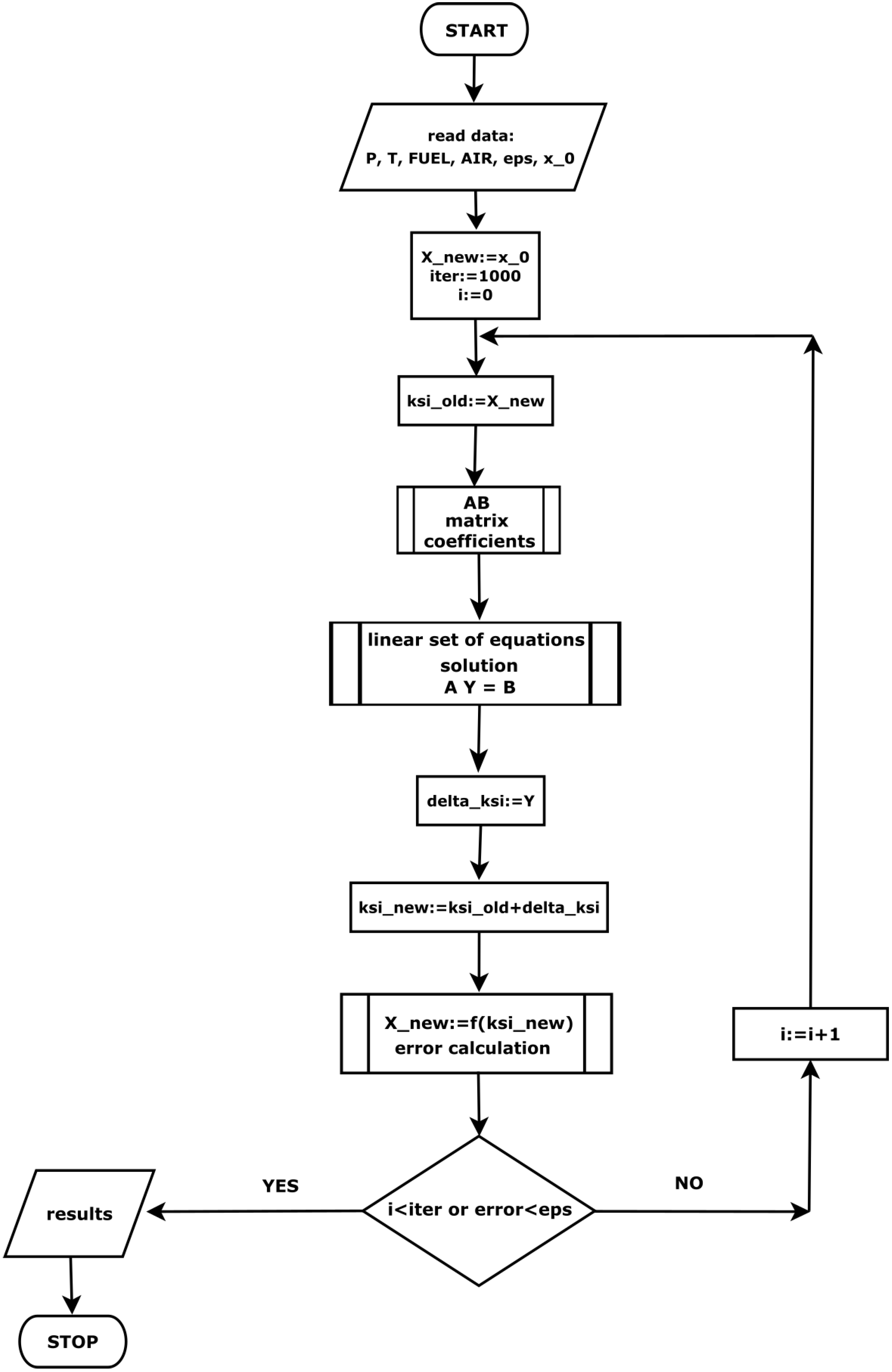
In this study, the Lagrangian multiplier method was adopted for the minimization of the Gibbs function. Implementing the approximation of solid fuels’ thermogravimetric data made it possible to apply the Gibbs method also for solid fuels. The in-house program for computing the equilibrium gas composition after the thermal treatment of biomass and waste was developed in the FORTRAN90 code.

2. Methodology

2.1. Equilibrium State and Gibbs Function Minimization

The conventional method for determining the equilibrium chemical composition of a mixture is based on the chemical reaction equation:
substrates ν i A i equilibrium state products ν j A j ,
where ν i are the stoichiometric coefficients and A i are the chemical components. The above can also be rewritten in the form:
a A + b B + c C + equilibrium d D + e E + f F +
The method based on reaction equations leads to the solution of a system of non-linear equations, which usually have many solutions, both real and complex. This, in turn, entails numerical instabilities, which makes the solving procedure much more difficult [11,12]. An alternative is undoubtedly the use of the Gibbs function minimization approach.
The equilibrium of a closed multi-component system under constant pressure and temperature, according to the second law of thermodynamics, brings down the problem to minimization of the Gibbs function:
G = U + p V T S + j = 1 n s μ j n j ,
where n s is the number of mixture components, n is the number of moles, and μ is the chemical potential. Differentiating the above, it can be written as:
d G = d U + p d V + V d p T d S S d T + j = 1 n s μ j d n j .
The heat supplied to the system can be defined according to the definition of entropy, which, for the thermodynamic equilibrium of the system, implies the fundamental equation:
d U = T d S p d V .
Combining Equations (4) and (5) leads to:
d G = V d p S d T + j = 1 n s μ j d n j .
The chemical potential μ j of the j-th component is an individual function of the characteristic variables (pressure, temperature) and composition (molar fraction) for each component:
μ j ( T ) = μ j 0 ( T ) + R T ln p j p 0 ,
where p j is the partial pressure of the gas component, μ j 0 ( T ) is the standard chemical potential (standard free enthalpy) of the j-th component, determined under standard conditions ( p 0 = 1013 hPa and T = 298 K). Considering the above and taking into account simple mathematical operations:
ln p j p 0 = ln p j p p p 0 = ln n j n t o t a l + ln p p 0 = ln ( n j ) ln ( n t o t a l ) + ln p p 0 ,
the chemical potential of the j-th component expressed by the Equation (7), is given by:
μ j ( T ) = μ j 0 ( T ) + R T ln ( n j ) R T ln ( n t o t a l ) + R T ln p p 0 ,
where n t o t a l is the total number of moles in the mixture in an equilibrium state:
n t o t a l = j = 1 n s n j .
For solids or liquids the chemical potential is only a function of temperature.
The method of minimizing the Gibbs function does not require knowledge of the reaction mechanism, only the assumption of what components are involved in it. Considering the processes of solid fuel thermal treatment as isobaric and isothermal, Equation (6) can be written in the form:
d G = j = 1 n s μ j d n j = j = 1 n s μ j 0 ( T ) + R T ln ( n j ) R T ln ( n t o t a l ) + R T ln p p 0 d n j .
The number of moles of each individual component depends on the initial elemental composition:
j = 1 n s a i j n j = b i , i = 1 , 2 , , n p ,
where b i denotes the number of moles of the i–th element in the system prior to chemical reactions, a i , j is the number of moles of the i-th element in the j-th substance, n p is the number of chemical elements considered. Equation (11) yields the following limitation:
φ i = j = 1 n s a i j n j b i = 0 .
Additional limitation results from the equation of mass conservation in the system, e.g., for oxidation or partial oxidation, the total mass of the system will be:
m t o t a l = m f u e l + m o x y g e n .
For pyrolysis, a process that takes place without access to oxygen, the mass of the oxidizer equals zero. The above equation can be represented by the sum of the masses of the specific components, thus:
i = 1 n s n i M i = m t o t a l ,
where M i is the molar mass of a given component expressed in [g/mol]. Additionally, the upper limit for the total number of moles in the system ( n t o t a l ) should follow the relationship:
j = 1 n s n j = n t o t a l j = 1 n s n j n t o t a l = 0 .

2.2. Lagrange Multipliers Method

The problem of determining the equilibrium composition of the mixture results in searching for the minimum of the Gibbs function, under the conditions defined by Equations (12) and (15). This issue can in turn be reduced to the optimization procedure using the Lagrange multipliers method, enriched with the number of unknowns corresponding to the number of variables. The Lagrange function in the considered case takes the form:
L = G + i = 1 n p + 1 λ i φ i ,
where λ i is the so-called Lagrange multiplier, the number of which, as aforementioned, results from the set limitations. The search for the function minimum leads to zeroing its partial derivatives, which in turn entails solving the following system of equations:
L n j = 0 , L λ i = 0
Taking into account the form of the Gibbs function, given by Equation (10), the following system of equations should be solved:
L n j = μ j ( T ) + i = 1 n p λ i φ i = 0 , j = 1 , , n s , L λ i = φ i = 0 , i = 1 , , n p + 1 ,
where n s is the number of components of the mixture, n p + 1 is the number of the system variables. The detailed form of the limitations set on the system is presented in the previous work [13].
The Lagrangian function with defined limitations takes the following form [13]:
L = i = 1 n s n C H μ i n i + i = 1 n C H μ C p i H q i n C p i H q i + i = 1 n p + 1 λ i φ i .
The transition from the minimization of the Gibbs function to the search for the minimum of the Lagrange function increases the number of unknowns, according to the system of Equation (18). In the analyzed case, a system of n s + n p + 1 equations with n s + n p + 1 unknowns should be solved, of which n s equations are non-linear. The number of unknowns takes into account not only the molar amounts of the components but also the values of the Lagrange coefficients and the total number of moles in the mixture. It is convenient to use Newton’s numerical method to determine these unknowns [14]. Non-linear system of equations in the form:
F ( X ) = 0 , X T = [ x 1 , x 2 , x 3 , , x n ] ,
can be solved iteratively:
X ( n + 1 ) = X ( n ) + δ X .
Using the Taylor series expansion of F ( X ) :
F ( X ( n + 1 ) ) = F ( X ( n ) + δ X ) = F ( X ( n ) ) + i = 1 n F ( X ( n ) ) x i δ x i + O ( δ X 2 ) = 0 ,
and neglecting terms of the second order, one derives at:
F ( X ( n + 1 ) ) F ( X ( n ) ) + i = 1 n F ( X ( n ) ) x i δ x i .
Taking into account the relationship (22), a system of linear equations is obtained due to corrections of the X vector, i.e., due to δ X . This allows for the simplification of the initial non-linear problem to the system of linear equations with unknown solution corrections:
i = 1 n F ( X ( n ) ) x i δ x i = F ( X ( n ) ) .
In order to simplify the calculations, new variables are substituted in the system of equations:
ξ i = ln n i n i δ ξ i = δ n i ,
for
i = 1 , , n s = CH 4 , CO , CO 2 , H 2 O , H 2 , O 2 , N 2 , i = 1 n CH C p i H q i ,
and
ξ = ln n t o t a l n t o t a l δ ξ = δ n t o t a l ,
π j = λ j R T R T δ π j = δ λ j , j = 1 , , n p + 1 .
After simple transformations, the final system of linear equations takes the form:
A Y = B ,
where the vector of unknowns is defined as:
Y T = [ δ ξ , δ π 1 , δ π 2 , δ π 3 , δ π 4 , δ π 5 , δ π 6 ] ,
and the coefficient matrix A and the free terms matrix B are functions of the number of moles of each component. The detailed forms of F ( X ( n ) ) , A, and B are given in [13].
The system (28) is therefore a system of linear equations due to the unknown corrections for the number of moles of the mixture δ ξ , and due to the corrections for the Lagrangian multipliers δ π j . By calculating these values, it is possible to iteratively determine the corrections for the number of moles of individual components, and thereby the solution sought:
ln n j ( n + 1 ) = ln n j ( n ) + ϵ δ ξ j n j ( n + 1 ) = n j ( n ) e ϵ δ ξ j ,
ln n t o t a l ( n + 1 ) = ln n t o t a l ( n ) + ϵ δ ξ n t o t a l ( n + 1 ) = n t o t a l ( n ) e ϵ δ ξ ,
λ i ( n + 1 ) R T = λ i ( n ) R T + ϵ δ π i λ i ( n + 1 ) = λ i ( n ) R T ϵ δ π i ,
where ϵ 0 , 1 is the so-called correction parameter determined empirically [9] used to obtain convergence. To further save computational time, the number of moles of each component is calculated only for specific values of the mole fraction of a given component, i.e., only for those X i values that are greater than a specified value [9], according to the equation:
ln n j n t o t a l = 18.420681 = SIZE SIZE = 18.420681
The value of ϵ is calculated according to the following scheme:
ϵ = min ( 1 , λ 1 , λ 2 ) ,
where parameters λ 1 and λ 2 are defined as:
λ 1 = 2 max 5 δ ξ , j = 1 n s δ ξ j , for ln n j n t o t a l > SIZE ,
λ 2 = min ln n j n t o t a l 9.2103404 δ ξ j δ ξ for ln n j n t o t a l SIZE and δ ξ j 0 .
It is also worth emphasizing that the method of Lagrange multipliers based on the Gibbs function is a universal method for determining the equilibrium composition of gases. Information on the composition of multi-component mixtures is one of the basic problems arising in the analysis of oxidation processes. As long as the composition of the fuel mixture is known, it is easy to predict the fractions and types of individual gaseous products of stoichiometric reactions. A problem may arise when there is no information about detailed reaction schemes, global or indirect.

2.3. Computation Procedure

To calculate the composition of the gas mixture under equilibrium conditions, the in-house numerical code was developed in the FORTRAN 90 programming language. A block diagram of this program is shown in Figure 1. The starting point is to load data such as fuel mass m f u e l , oxidizer mass m a i r , temperature T and process pressure p, calculation error ϵ and initial solution x 0 , which is the number of moles of components relative to the total number of moles; x 0 is a one-dimensional array whose individual elements represent mole fractions. The sum of these elements gives a value equal to unity. In the first stage of calculations, the initial value is assigned as the searched solution, for which the correction is determined. In subsequent iterative steps, this solution is taken from the previous step. Then, new variables ξ are determined which are the basis for computing the values of the matrix coefficients of the linear Equation (28), whose unknowns are the sought corrections (29). These unknowns are obtained by solving a system of linear equations by decomposing the A matrix into a lower and an upper matrix (Lower Upper Decomposition). Knowing the appropriate corrections, a new solution is derived. Further, through appropriate transformations, the values of the moles of individual components are obtained. The iterative process is performed until the assumed calculation error is reached or the set number of iterations is exceeded.
The values of standard chemical potentials, necessary to perform the minimization procedure, are computed using the formula:
μ i 0 ( T ) = h i 0 ( T ) T s i 0 ( T ) ,
the specific heats required for the determination of enthalpies of individual components are defined as [15]:
c p x , i T = a i + b i T + c i T 2 + d i T 2 , c p , i T = c p x , i / M i ,
In the above equations c p x , c p , and M stand for specific heat, molar specific heat, and molar mass, respectively. Individual coefficients in Equation (35) come from works [15,16,17] and they are listed in Table 1.
The temperature-dependent values of chemical potentials and molar specific heats are graphically presented in Figure 2 and Figure 3. Both molar specific heats and chemical potentials strongly depend on temperature. With the increase of this parameter, the molar specific heat values increase (except for benzene, for which a slight decrease in this value occurs at higher temperatures), whereas the values of chemical potentials decrease. It is also worth noting that heavier hydrocarbons have values of c p x 2 to 5 times higher than other considered chemical species (see Figure 2 and Figure 3).

3. Results

Calculations and analyses were carried out for three types of biomass: pine, olive residues, and wood chips, as well as for coal. The physical properties of these fuels are presented in Table 2 [18,19].
Comparing the above data, it can be seen that the analyzed types of biomass contain more volatiles, about 3 times higher than coal. Thus, the biomass fixed carbon content is more than 2 to 5 times lower than that of coal. In addition, coal contains much more ash, from about 2 times more than olive residues to more than 40 times more than wood chips. The moisture content for the two types of considered biomass is approximately 10% and as much as approximately 35% (wood chips), while for coal this value is much lower and amounts to approximately 1%. As a result, biomass has a lower content of carbon (C) and a much higher content of oxygen (O), compared to coal.
A key input parameter is the amount of released gases at a given temperature, which is determined based on the fuel mass loss curve as a function of temperature. Mass loss functions were obtained by approximating the thermogravimetric data [18,20] by the error function [21]. The TGA experiments were performed in atmospheric pressure conditions with nitrogen as a carrier gas with a mass flow of 100 mL/min and with a heating rate of raw samples of 10 K/min.
Percentage mass loss of biomass samples referred to as the mass loss progress function, and defined as a ratio of instantaneous to initial mass of a sample, is described in the temperature range 400 ÷ 1300 K by the function:
Z = 100 D T A 2 1 + e r f T B 2 C .
In the case of coal, this function is approximated in two ranges of temperature as follows:
Z T 1 = 100 a 1 2 1 + e r f T b 1 2 c 1 , T 273 , 573 K ,
Z T 2 = 100 d T a 2 2 1 + e r f T b 2 2 c 2 a 1 , T 573 , 1173 K .
Values of all coefficients for considered fuel samples are given in Table 3.
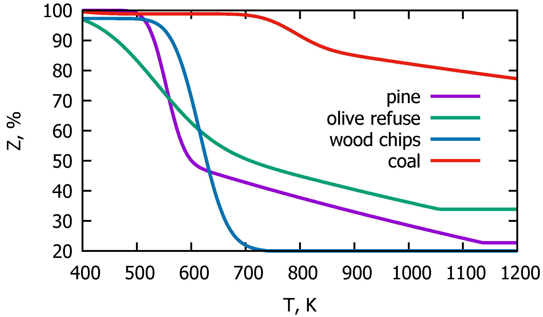
Approximation of the TGA experimental results for mass loss of the analyzed samples is presented in Figure 4.
As can be seen, all lines have a similar character, i.e., with an increase in the temperature of the raw material, the mass of the sample decreases. Figure 4 shows the curves for the devolatilization process of the different types of fuels. Materials such as pine and wood chips behave similarly. The most intensive devolatilization process for those fuels takes place at a temperature of about 600 K. These curves are slightly shifted from each other but both of them reach the limit value of about 20% at 1200 K. This value results from the content of volatiles, which for these materials is approximately 80%. Olive residues behave a little differently demonstrating much slower dynamics of mass loss. Despite this, the most intensive pyrolysis process of this material falls within the same temperature range as in the case of other types of biomass, but the release of gases is distributed over almost the entire analyzed temperature range. In addition, olive residues contain fewer volatiles, which amount to about 67% of the total weight, and this value is reached at 1200 K.
Generally, for biomass, the temperature of the most intensive gas release is much lower than in the case of coal, which is seen in Figure 4. The ratio of biomass volatile content to fixed carbon content exceeds 4, while for coal the same ratio is below 1. The impact of this ratio on the devolatilization process can be seen in the presented thermogravimetric graphs. For biomass, the release of volatile substances mainly occurs immediately after the sample drying. The latter takes place in the temperature range from about 323 to 373 K, while pyrolysis occurs between 460 and 700 K. The most intensive mass loss observed for coal takes place at a temperature around 800 K (Figure 4, red curve). Moreover, the red curve decreases down to a limit value of 22%, which is the value of coal’s volatile content.
Comparing the thermogravimetric curves of biomass and coal, it can therefore be concluded that the mass loss of biomass is greater than for coal due to the higher volatile content in comparison to coal. The high ratio of volatiles to fixed carbon also proves the dominant form of combustion, which in the case of biomass is gas oxidation, not solid-phase oxidation. The coal’s thermogram indicates a less intense release of volatiles than in the case of biomass and, thereby, highly heterogeneous gas–solid oxidation reactions due to the much lower content of volatiles and higher content of fixed carbon. Comparing the behavior of biomass and coal during the heating process, it can be clearly stated not only that biomass losses its mass much faster but also that the change in its mass is greater.
The graphs in Figure 5 and Figure 6 show numerical results of the composition of pyrolitic gas from the thermal treatment of the analyzed solid fuels. 
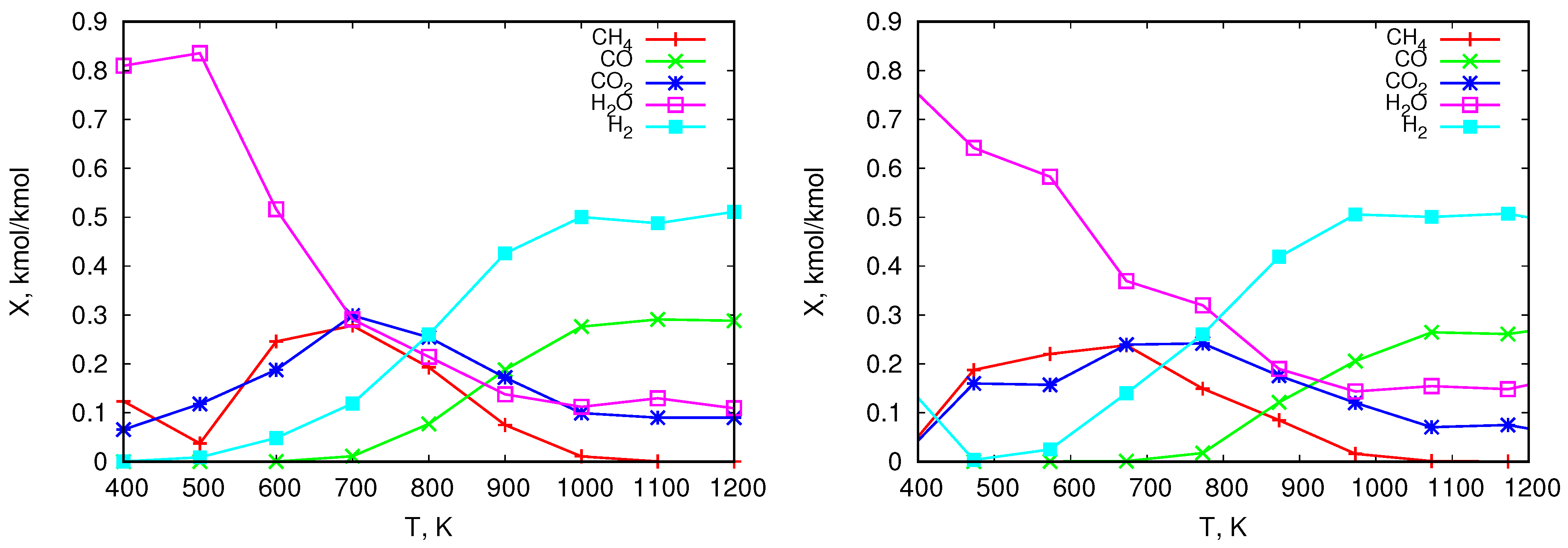
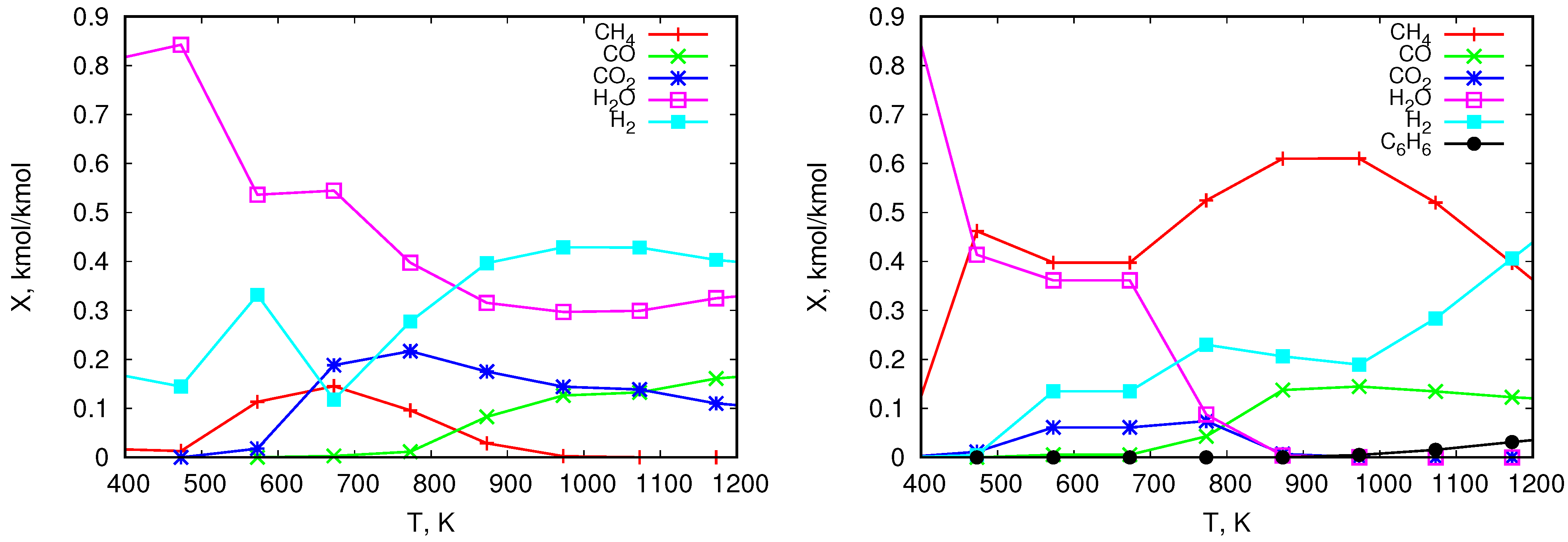
Figure 5 shows the distribution of the mole fractions of individual components released during the heating of pine (left) and olive residues (right). The same is illustrated for wood chips in Figure 6 on the left and for coal on the right. The obtained results show that for all analyzed types of biomass the mole fractions of CH 4 reach their maximum values. Depending on the type of biomass these values range from approximately 10% to approximately 30%. They are reached at a temperature of approximately 700 K, and then they decrease to zero at about 1000 K. On the other hand, the mole fraction of H 2 released from biomass increases with increasing temperature to about 50%. As expected, due to the high content of moisture and oxygen in biomass, the content of H 2 O in the pyrolysis gas is high and varies from values close to 100% (which is related to moisture evaporation) to values ranging between 10% and 30%. In addition, the CO level increases with rising temperature to the value of approximately 20–30%. In the case of coal, a much higher content of methane is obtained compared to biomass. Its maximum value is shifted to the region of higher temperatures to about 950 K. The CO content, similarly as for biomass, increases to about 10%. The share of CO 2 compared to biomass is smaller (about 20% for biomass and about 5% for coal). The water content in the pyrolysis gas from coal results from moisture evaporation, and its share at higher temperatures is much smaller than in the case of biomass. Gas from coal is also characterized by a lower content of H 2 , its maximum appears at higher temperatures and is about 40%. This lower level of hydrogen in gas from coal may come from the fact that the H content in coal, in comparison to biomass, is smaller (see Table 2). Additionally, at higher temperatures H combines with C and produces higher hydrocarbons ( C 6 H 6 ), which does not take place in the case of biomass. This can also affect lower H 2 content in gas from coal in comparison to gas from biomass.

4. Model Verification

In order to check the correctness of the equilibrium model, the predicted pyrolysis gas compositions were compared with the numerical results obtained by other authors and with the available experimental results. Due to the lack of relevant data on the composition of considered raw materials, substances of similar composition were used for comparison (sawdust [22] and palm fibers [23]). The properties of those materials are presented in Table 4. The juxtaposition of these results with the literature results indicates the same, in terms of quality, nature of the biomass pyrolysis process (Table 5). The mole fractions of CH 4 , CO 2 , and H 2 O in the pyrolysis gas from biomass decrease, while those of CO and H 2 increase.
Table 5 presents the results of this and other authors’ computations for syngas composition from the biomass gasification process. For the comparative study, the air-to-fuel ratio of 2 was assumed (the stoichiometric air-to-fuel ratio for the given composition is 5.77), so that the level of volumetric amount of N 2 in the syngas is similar in both analyzed cases (this is not clear from the information provided in the article [22]). The trends are the same as for pyrolysis, namely the molar fractions of CH 4 and CO 2 decrease, whereas CO and H 2 increase. The observed differences, especially in the amount of H 2 O , result from the lack of appropriate data in the cited work, which were needed for complete computation (sawdust, see Table 4). The proposed numerical software treats only special elemental and technical analyses as input, that is a technical analysis of raw material (as received) and chemical elemental analysis of dry material (dry basis). To fill this data it was assumed that sawdust fuel has the same physical properties as cited palm fibers.
A data comparison shows that the content of H 2 O obtained in the present study is higher. This results from the fact that in the case of Khadse, A. et al.’s analysis [22], the dry fuel was taken into account. Dry fuel consists of a lesser amount of O, so the content of CO 2 in syngas should be lower, as is seen in the presented data. Carbon dioxide content in the authors’ computation is much higher than for Khadse, A. et al. [22].
Table 6 and Table 7 present the numerical and experimental results for syngas composition from the thermal treatment of biomass.
The trends are the same as in the previous cases, namely the mole fraction of CO 2 is decreasing, while for CO and H 2 mole fractions are increasing. The mole fractions of CO 2 and H 2 also agree qualitatively with the data presented in work [27].
The differences between the equilibrium numerical results come from the proposed approaches. The authors’ method does not include any solid specie for thermal conversion, while in the paper of Yan, R. et al. (2005) [23], the composition of syngas is calculated including also C as an input solid chemical specie. In the proposed method, only the volatiles undergo the chemical reactions as a gaseous phase, which consists of a lesser amount of C. The input carbon content in the Gibbs analysis is thus reduced by the value of the fixed carbon as assumed that it is composed of pure C.
It is worth noticing that when comparing the numerical results with the experimental results (Table 7), the predicted mole fraction of CO remains more or less at the same level.
This is not the case as regards CH 4 . The calculations of the present study show a clear decrease in its content in the gas mixture with increasing process temperature. In straw pyrolysis experiments, as well as for wood, there is an initial slight increase and then a slight decrease in the content of CH 4 . Differences between the gas composition obtained from these calculations and those from the measurements result from the fact that the numerical analysis took into account the content of moisture, which was not included in the experiments (dry straw pyrolysis [24], pyrolysis of dry wood [25,26]). Additionally, in the equilibrium devolatilization case it was assumed that all volatiles available for decomposition at a certain temperature were released in the process, which does not occur in reality. The sample residence time is often too short to account for 100% of decomposition at a given temperature. Moreover, in the proposed approach, it was assumed that all chemical elements are released homogeneously, i.e., at a given temperature, their mass composition is always the same and determined by the chemical elemental analysis of raw material. In fact, their release is also a function of temperature [28,29]. All mentioned issues do not allow for quantitative verification of these results. Nevertheless, the proposed computation method is a quick and simple tool for determining the qualitative composition of pyrolysis gas, which can be used for the initial estimation of operating conditions and geometrical parameters of devices for the thermal treatment of solid fuels, as well as for analyzing the possibility of using generated gases in other devices, such as boilers, engines, or other plants powered by gas fuels.

5. Summary

This work aimed to predict gas composition released during the heating of biomass fuels. For this purpose, a method based on the second law of thermodynamics was used, which allowed for determining the equilibrium composition of pyrolysis gas at a given temperature and pressure. The elemental and technical analysis of the solid fuels and the approximation of thermogravimetric data were used as input for the Lagrange multipliers procedure, which was developed and implemented in a FORTAN90 language. The in-house software was tested and validated. It was shown that the composition of the mixture depends on the process temperature and the fuel type. For each considered biomass-type fuel, a decrease in the water vapor content and an increase in hydrogen and carbon monoxide content were obtained with an increase in temperature. The mole fractions of methane and carbon dioxide in the pyrolysis gas mixture initially increased and then decreased with increasing temperature. The obtained difference between the composition of gas from biomass and coal results from the chemical composition of these raw materials. In the case of biomass, larger mole fractions of water vapor, hydrogen, and carbon dioxide were obtained, whereas methane and carbon monoxide were smaller. In the case of coal, a little amount of higher hydrocarbons were observed. The obtained results agree qualitatively with the data available in the literature. The presented simple and fast method for predicting equilibrium gas composition can support the design and optimization of thermal conversion devices for solid fuels. The developed software can also be useful for analyzing the possibility of supplying other devices such as boilers, engines, or other plants with alternative gas fuels, especially those derived from municipal solid waste or sewage sludge. These raw materials are characterized by a highly differentiated chemical composition related to the source and place of their origin. Obtaining the proper parameters of their combustion process, as well as the control of the oxidation reactions for efficiency and clean heat and power generation, could be very difficult. The prediction of pyrolysis gas composition under variable operational parameters could be very useful at the first stage of the design process. Moreover, such predictions are very valuable for more complex CFD computation, and they could be used as input data for full 3D simulations.

Author Contributions

Conceptualization, D.K.; methodology, D.K. and I.W.-Ś.; software, I.W.-Ś.; validation, I.W.-Ś.; formal analysis, D.K. and I.W.-Ś.; investigation, I.W.-Ś.; resources, D.K. and I.W.-Ś.; data curation, I.W.-Ś.; writing—original draft preparation, I.W.-Ś.; writing—review and editing, I.W.-Ś. and D.K.; visualization, I.W.-Ś.; supervision, D.K.; project administration, D.K.; funding acquisition, D.K. All authors have read and agreed to the published version of the manuscript.

Funding

This research received no external funding.

Data Availability Statement

Data is contained within the article.

Conflicts of Interest

The authors declare no conflict of interest.

Abbreviations

The following abbreviations s are used in this manuscript:
A liner set of equation coefficients matrix
B liner set of equation coefficient matrix
C p H q higher-hydrocarbons
c p specific heat, J/kgK
c p x molar specific heat, J/molK
CH 4 methane
C 2 H 6 ethane
C 4 H 10 butane
C 6 H 6 benzene
CO carbon oxide
CO 2 carbon dioxide
EUEuropean Union
GGibbs free energy, J
H 2 hydrogen
H 2 O vapour
jfor substrates
LLagrange function,  J
mmass, kg
Mmolar mass, kg/kmol
nnumber of moles, mol
N 2 nitrogen
n p number of chemical elements
n s number of mixture components
O 2 oxygen
ppressure, Pa
p 0 standard pressure, Pa
p j gas partial pressure, Pa
Runiversal gas constant, 8.314 J/molK
Sentropy, J/K
Ttemperature, K
TGAthermogravimetric analysis
Uinternal energy, J
Vvolume, m 3
X vector of unknowns
δ X vector of corrections for unknowns
Y renamed vector of unknowns
ϵ correction parameter
λ Lagrange multiplier or parameter
μ chemical potential, J/mol
μ j 0        standard Gibbs chemical potential, J/mol
π renamed unknown
φ limitation
ξ renamed unknown

References

  1. Polesek-Karczewska, S.; Turzyński, T.; Kardaś, D.; Heda, Ł. Front velocity in the combustion of blends of poultry litter with straw. Fuel Proc. Technol. 2018, 176, 307–315. [Google Scholar] [CrossRef]
  2. Kantorek, M.; Jesionek, K.; Polesek-Karczewska, S.; Ziółkowski, P.; Badur, J. Thermal utilization of meat and bone meals. Performance analysis in terms of drying process, pyrolysis and kinetics of volatiles combustion. Fuel 2019, 254, 115548. [Google Scholar] [CrossRef]
  3. Teh, J.S.; Teoh, Y.H.; How, H.G.; Sher, F. Thermal Analysis Technologies for Biomass Feedstocks: A State-of-the-Art Review. Processes 2021, 9, 1610. [Google Scholar] [CrossRef]
  4. Jeon, H.; Park, J.-Y.; Lee, J.W.; Oh, C.-H.; Kim, J.-K.; Yoon, J. Fractional Composition Analysis for Upgrading of Fast Pyrolysis Bio-Oil Produced from Sawdust. Energies 2022, 15, 2054. [Google Scholar] [CrossRef]
  5. Kazakov, A.; Frenklach, M. Reduced Version of GRI-MECH 1.2, 22 Species. 1994. Available online: http://www.me.berkeley.edu/drm/ (accessed on 10 February 2015).
  6. Smith, G.P.; Golden, D.M.; Frenklach, M.; Moriarty, N.W.; Eiteneer, B.; Goldenberg, M.; Bowman, C.T.; Hanson, R.K.; Song, S.; Gardiner, W.C., Jr.; et al. GRI-MECH 3.0. 1999. Available online: http://www.me.berkeley.edu/gri_mech/ (accessed on 10 February 2015).
  7. Starik, A.M.; Titova, N.S.; Sharipov, A.S.; Kozlov, V.E. Syngas Oxidation Mechanizm. Combust. Explos. Shock Waves 2010, 40, 491–506. [Google Scholar] [CrossRef]
  8. Ścia̧żko, M. Models of Coal Classification in Thermodynamic and Kinetic Terms; Wydawnictwa AGH: Kraków, Poland, 2010. (In Polish) [Google Scholar]
  9. Gordon, S.; McBride, B.J. Computer Program for Calculation of Complex Chemical Equilibrium; NASA Lewis Research Center: Cleveland, OH, USA, 1994; Chapter 3; pp. 13–18. [Google Scholar]
  10. Otto, C.; Kempka, T. Synthesis Gas Composition Prediction for Underground Coal Gasification Using a Thermochemical Equilibrium Modeling Approach. Energies 2020, 13, 1171. [Google Scholar] [CrossRef] [Green Version]
  11. Oran, E.S.; Boris, J.P. Numerical Simulation of Reactive Flows, 2nd ed.; Cambridge University Press: Cambridge, UK, 2001. [Google Scholar]
  12. Hirsch, C. Numerical Computation of Internal and External Flows; Computational Methods for Inviscid and Viscous Flows; Jorn Wiley & Sons: Hoboken, NJ, USA, 1994; Volume 2. [Google Scholar]
  13. Wardach-Święcicka, I. Modeling of Physicochemical Processes Occurring in a Single Solid Fuel Particle in a Stream of Hot Gases. Ph.D. Thesis, IMP PAN, Gdańsk, Poland, 2017. [Google Scholar]
  14. Press, W.H.; Teukolsky, S.A.; Vetterling, W.T.; Flannery, B.P. Numerical Recipes in Fortran 77, 2nd ed.; Cambridge University Press: Cambridge, UK, 1992. [Google Scholar]
  15. Demichowicz-Pigoniowa, J. Physico-Chemical Calculations; PWN: Warsaw, Poland, 1984. (In Polish) [Google Scholar]
  16. Turns, S.R. Introduction to Cmbustion–Concepts and Applications; McGraw–Hill, Inc.: Singapore, 1996. [Google Scholar]
  17. Material Properties. Available online: http://www.engineeringtoolbox.com/ (accessed on 6 February 2019).
  18. Ściążko, M. (Ed.) Development of a Model of Pressure Generation by a Bed of Thermally Plasticized Coal Packed-Bed; Technical Report; ITPE: Zabrze, Poland, 2005. (In Polish) [Google Scholar]
  19. Senneca, O. Kinetics of pyrolysis, combustion and gasification of three biomass fuels. Fuel Process. Technol. 2007, 88, 87–97. [Google Scholar] [CrossRef]
  20. Kardaś, D.; Kluska, J.; Polesek-Karczewska, S. Introduction to the Issues of Biomass Gasification; Wydawnictwa Instytytu Maszyn Przepływowych PAN: Gdańsk, Poland, 2014. (In Polish) [Google Scholar]
  21. Kardaś, D.; Polesek-Karczewska, S.; Wardach, I.; Kamiński, T.; Ochrymiuk, T. Transient one dimensional modelling of pyrolysis and combustion processes of biomass and coal. In Proceedings of the 8th European Conference on Industrial Furnaces and Boilers, Vilamoura, Portugal, 25–28 March 2008. [Google Scholar]
  22. Khadse, A.; Parulekar, P.; Aghalayam, P.; Ganesh, A. Equilibrium model for biomass gasification. Adv. Energy Res. 2006, AER-2006, 106–112. [Google Scholar]
  23. Yan, R.; Yang, H.; Chin, T.; Liang, D.T.; Chen, H.; Zheng, C. Influence of temperature on the distribution of gaseous products from pyrolyzing palm oil wastes. Combust. Flame 2005, 142, 24–32. [Google Scholar] [CrossRef]
  24. Werther, J.; Saenger, M.; Hartge, E.-U.; Ogada, T.; Siagi, Z. Combustion of agricultural residues. Prog. Energy Combust. Sci. 2000, 26, 1–27. [Google Scholar] [CrossRef]
  25. Kardaś, D.; Kluska, J.; Klein, M.; Kazimierski, P.; Heda, Ł. Experimental and Theoretical Issues of Biomass and Waste Pyrolysis; Internal Report; IMP PAN: Gdańsk, Poland, 2013; unpublished. [Google Scholar]
  26. Kardaś, D.; Kluska, J.; Klein, M.; Kazimierski, P.; Heda, Ł. Theoretical and Experimental Aspects of Wood and Waste Pyrolysis; Wydawnictwo Uniwersytetu Warmińsko-Mazurskiego: Olsztyn, Poland, 2014. (In Polish) [Google Scholar]
  27. Basu, P. Biomass Gasification, Pyrolysis and Torrefaction, Second Edition: Practical Design and Theory; Elsevier Inc.: Amsterdam, The Netherlands, 2013. [Google Scholar]
  28. Ahmed, A.; Bakar, M.S.A.; Sukri, R.S.; Hussain, M.; Farooq, A.; Moogi, S.; Park, Y.-K. Sawdust pyrolysis from the furniture industry in an auger pyrolysis reactor system for biochar and bio-oil production. Energy Convers. Manag. 2020, 226, 113502. [Google Scholar] [CrossRef]
  29. Yang, H.; Huang, L.; Liu, S.; Sun, K.; Sun, Y. Pyrolysis process and characteristics of Products from Sawdust Briquettes. BioResources 2016, 11, 2438–2456. [Google Scholar] [CrossRef]
Figure 1. Block diagram of FORTRAN program code for determining the equilibrium composition of the gas mixture.
Energies 16 01147 g001
Figure 2. Values of chemical potentials of individual gas components vs. temperature.
Energies 16 01147 g002
Figure 3. Molar specific heat values of individual gas components vs. temperature.
Energies 16 01147 g003
Figure 4. Mass loss of the fuel samples during heating-approximation of the TGA measurements.
Energies 16 01147 g004
Figure 5. Equilibrium composition of gases released in the pyrolysis process of pine (left) and olive residues (right)—mole fractions.
Energies 16 01147 g005
Figure 6. Equilibrium composition of gases released in the pyrolysis process of wood chips (left) and coal (right)—mole fractions.
Energies 16 01147 g006
Table 1. Polynomial coefficients for determining the molar specific heats, based on [15,16,17].
a b × 10 3 c × 10 6 d × 10 5
Component J / molK J / molK 2 J / molK 3 JK / mol
CH 4 14.3274.81−17.430
CO 28.424.100−0.46
CO 2 44.159.040−8.54
H 2 O 30.1311.3000
H 2 27.157.50−1.490
O 2 36.170.840−4.31
N 2 27.834.1800
C 2 H 6 5.75175.20−57.870
C 6 H 6 −24.86413.44−182.210
C 4 H 10 18.23303.60−92.680
Table 2. Properties of the analyzed fuels—technical and elemental analysis, %weight.
Fuel TypePineOlive ResiduesWood ChipsCoal
technical analysis, as received
moisture10.313.134.91.0
volatiles69.256.351.623.0
fixed carbon19.426.213.367.8
ash1.14.40.28.2
chemical analysis, dry basis
C48.551.847.382.8
H6.15.56.14.3
N0.21.30.22.0
O44.336.346.02.6
ash0.95.10.48.3
Table 3. Coefficients of mass loss function Z for analyzed fuel samples, based on [21].
PineOlive ResiduesWood Chips
A15.823218.8730−52.7296
B552.9960517.3830615.3150
C26.310187.956839.6230
D2.76162.61600.9035
Coal
a 1 1.5230
a 2 35.7304
b 2 780.8230
c 2 49.2996
d 2 1.6506
b 1 413.7940
c 1 39.5500
Table 4. Properties of biomass—technical and chemical elemental analysis, %weight.
Fuel TypePineSawdustPalm Fibres
Seneca O. (2007) [19]Khadse, A. et al. (2006) [22]Yan, R. et al. (2005) [23]
technical analysis, as received
moisture10.30n.d.6.56
volatiles69.20n.d.76.00
fixed carbon19.40n.d.12.50
ash1.10n.d.4.94
chemical elemental analysis, dry basis
C48.5052.2850.30
H6.105.207.07
N0.200.471.05
O44.3040.8536.30
ash0.901.205.28
Table 5. Predictions of equilibrium models for biomass gasification process—molar fractions, %.
SawdustSawdust
This StudyKhadse, A. et al. (2006) [22]
T [K]80090010008009001000
CH 4 1.190.120.012.51.50.7
CO 4.348.3312.084.514.526.5
CO 2 20.0717.9015.2814.510.04.0
H 2 O 11.5211.2211.439.15.02.0
H 2 10.2312.7013.4010.014.517.2
N 2 52.6649.7347.8059.454.549.6
Table 6. Predictions of equilibrium models for pyrolysis gas composition from palm—molar fractions, %.
PalmPalm
This StudyYan, R. et al. (2005) [23]
T [K]80090010008009001000
CH 4 39.3323.0610.4315.09.05.0
CO 14.3733.3541.262.012.030.0
CO 2 23.927.851.4512.010.08.0
H 2 O 5.413.281.0327.020.011.5
H 2 16.0331.6945.1927.043.066.0
N 2 0.940.770.65<0.1<0.1<0.1
Table 7. Gas composition (molar fractions %) from biomass pyrolysis process: numerical and experimental results.
Numerical ResultsExperimental Results
PineStrawStrawWood
This StudyWerther, J. et al. (2000) [24]Kardaś, D. et al. (2013) [25]Kardaś, D. et al. (2014) [26]
T [K]7238731023117387310231173873102311737231173
CH 4 26.2710.700.590.0210.012.57.010.012.57.010.017.0
CO 1.7615.3728.4031.1522.023.040.015.025.035.043.022.0
CO 2 29.6719.979.306.7835.027.518.045.025.021.026.020.0
H 2 15.3138.7950.1648.9220.024.035.028.029.032.05.033.0
Disclaimer/Publisher’s Note: The statements, opinions and data contained in all publications are solely those of the individual author(s) and contributor(s) and not of MDPI and/or the editor(s). MDPI and/or the editor(s) disclaim responsibility for any injury to people or property resulting from any ideas, methods, instructions or products referred to in the content.

