
A Fault Identification Method for Metal Oxide Arresters Combining Suppression of Environmental Temperature and Humidity Interference with a Stacked Autoencoder

Abstract
:1. Introduction
- (1)
- A functional relationship model between resistive current and environmental temperature and humidity is established to mitigate the impact of environmental temperature and humidity on the resistive current of an MOA. A method for suppressing environmental temperature and humidity interference using weighted nonlinear surface modeling is proposed. This method normalizes the resistive current to the reference temperature and humidity, resulting in a reduction in environmental interference with the resistive current.
- (2)
- An MOA fault identification method combining the suppression of environmental temperature and humidity interference with a stacking automatic encoder is proposed. Firstly, the MOA resistive current is suppressed by environmental temperature and humidity interference, and then the SAE classification algorithm is used to classify the suppressed resistive current, thereby achieving MOA fault identification.
- (3)
- The effectiveness of the MOA fault recognition method combining suppression of environmental temperature and humidity interference with a stacking automatic encoder is verified by comparison with several commonly used classification algorithms under three conditions: not considering environmental temperature and humidity, feature fusion of environmental temperature and humidity with resistive current, and suppression of environmental temperature and humidity interference.
2. Methods
2.1. General Framework
2.2. A Method of Environmental Temperature and Humidity Interference Suppression
| Algorithm 1 Temperature and humidity interference suppression algorithm. |
| Model: |
| Require: Input N MOA original data (Ir, t, h) and initial value b(0)= [b0(0), b1(0), …, b7(0)]T |
| for i←0 to K do for j←1 to N do Calculate the error between the fitted value and the truth value of Ir |
| if then Updated b(i) else i = k Obtain b(k)= [b0(k), b1(k), …, b7(k)] |
| Solve i.e., Solve |
| Obtain |
| return . |
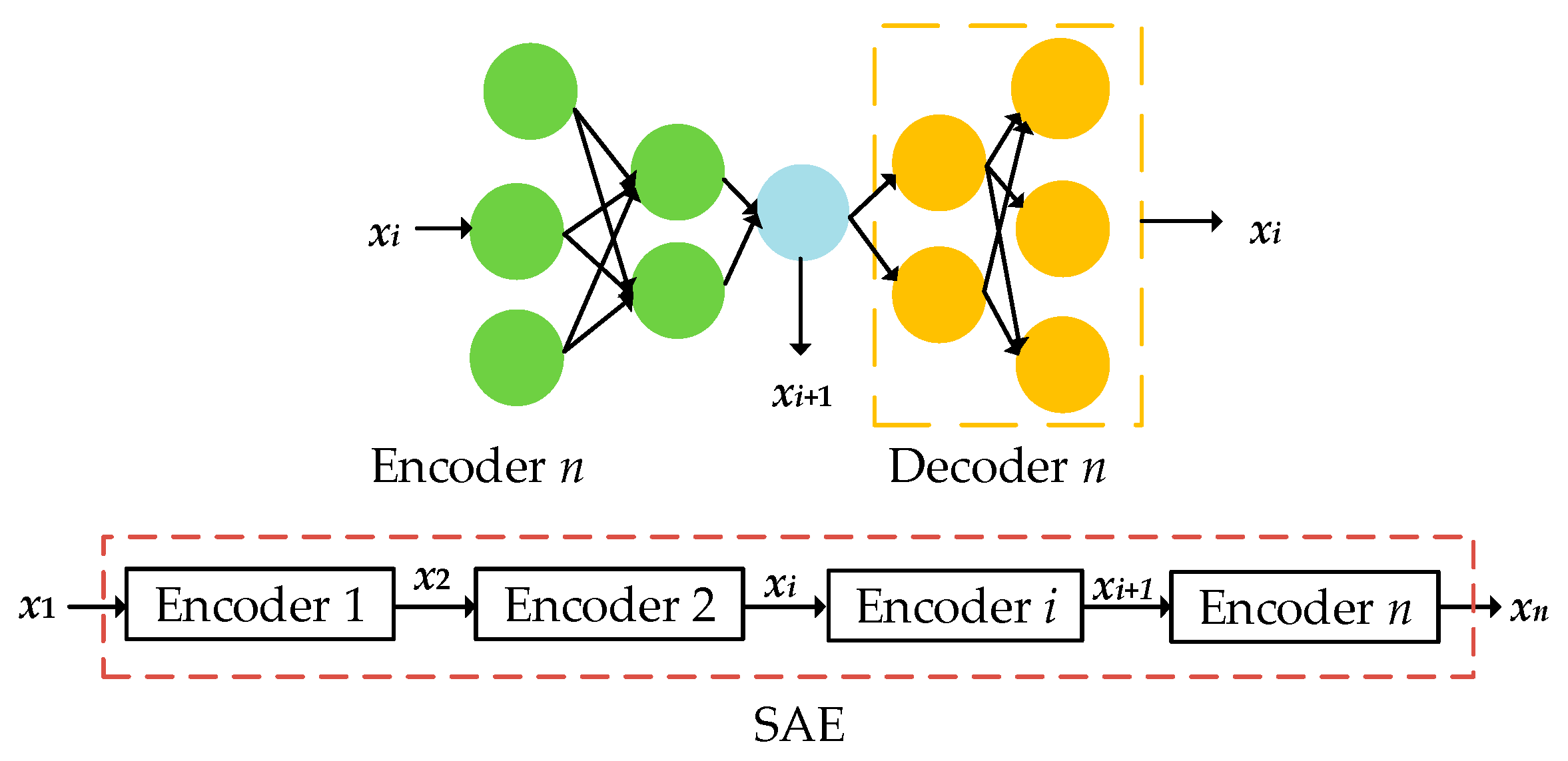
2.3. SAE
| Algorithm 2 SAE. |
| Require: Input the data x1 to be classified obtain x2 with a vector length of 30 obtain x3 with a vector length of 3 obtain y2 with a vector length of 30 Output: Numbers representing categories. |
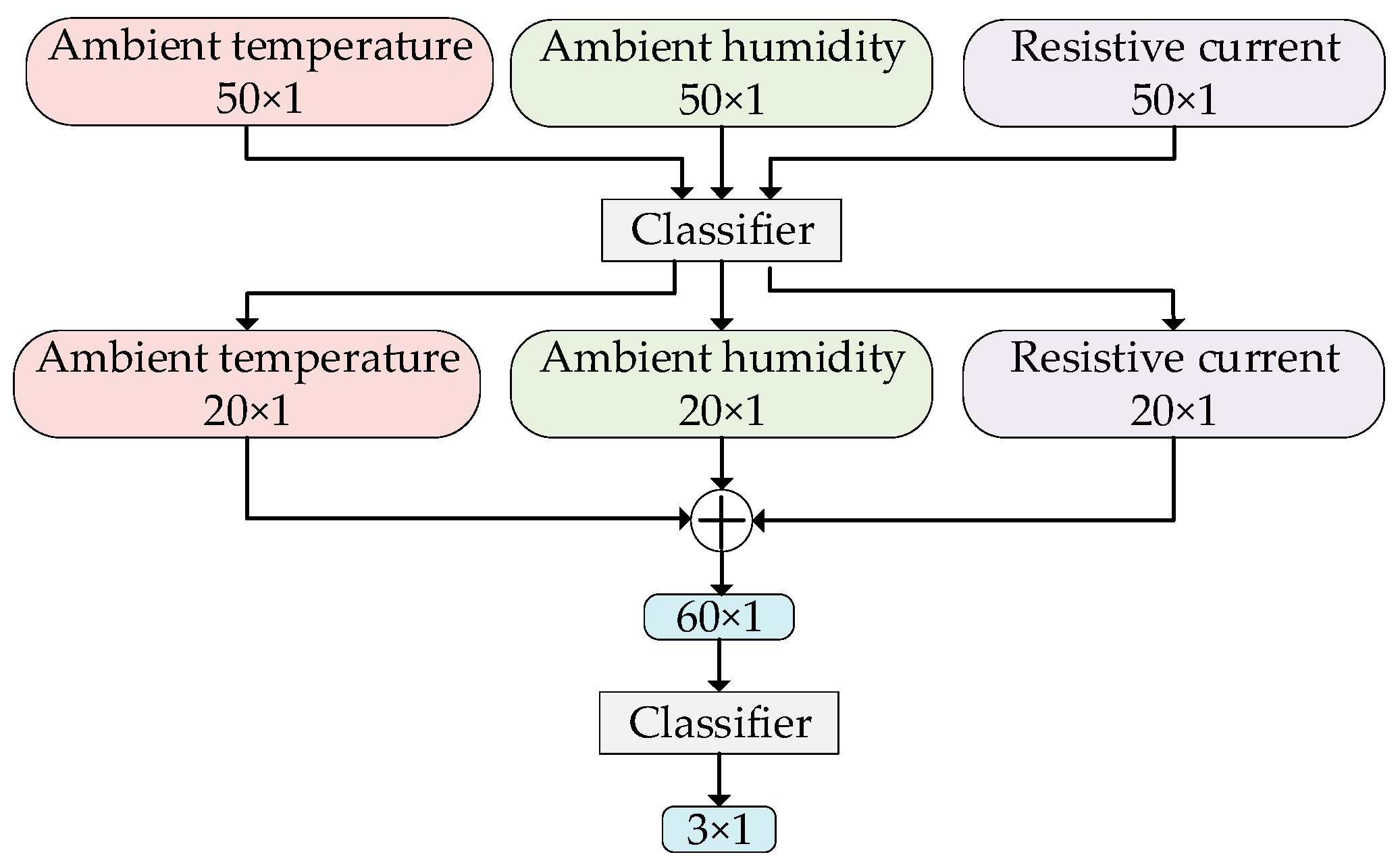
2.4. Comparison Algorithm: Feature Fusion
3. Results
3.1. Data Samples
3.2. Model Evaluation Indicators
- (1)
- Recall
- (2)
- Precision
- (3)
- Accuracy
- (4)
- F1-score
- (5)
- Kruskal–Wallis test
3.3. Comparison of Results before and after Suppression of Environmental Temperature and Humidity Interference
3.4. MOA Classification Algorithm Combining Suppressing Environmental Temperature and Humidity Interference with SAE
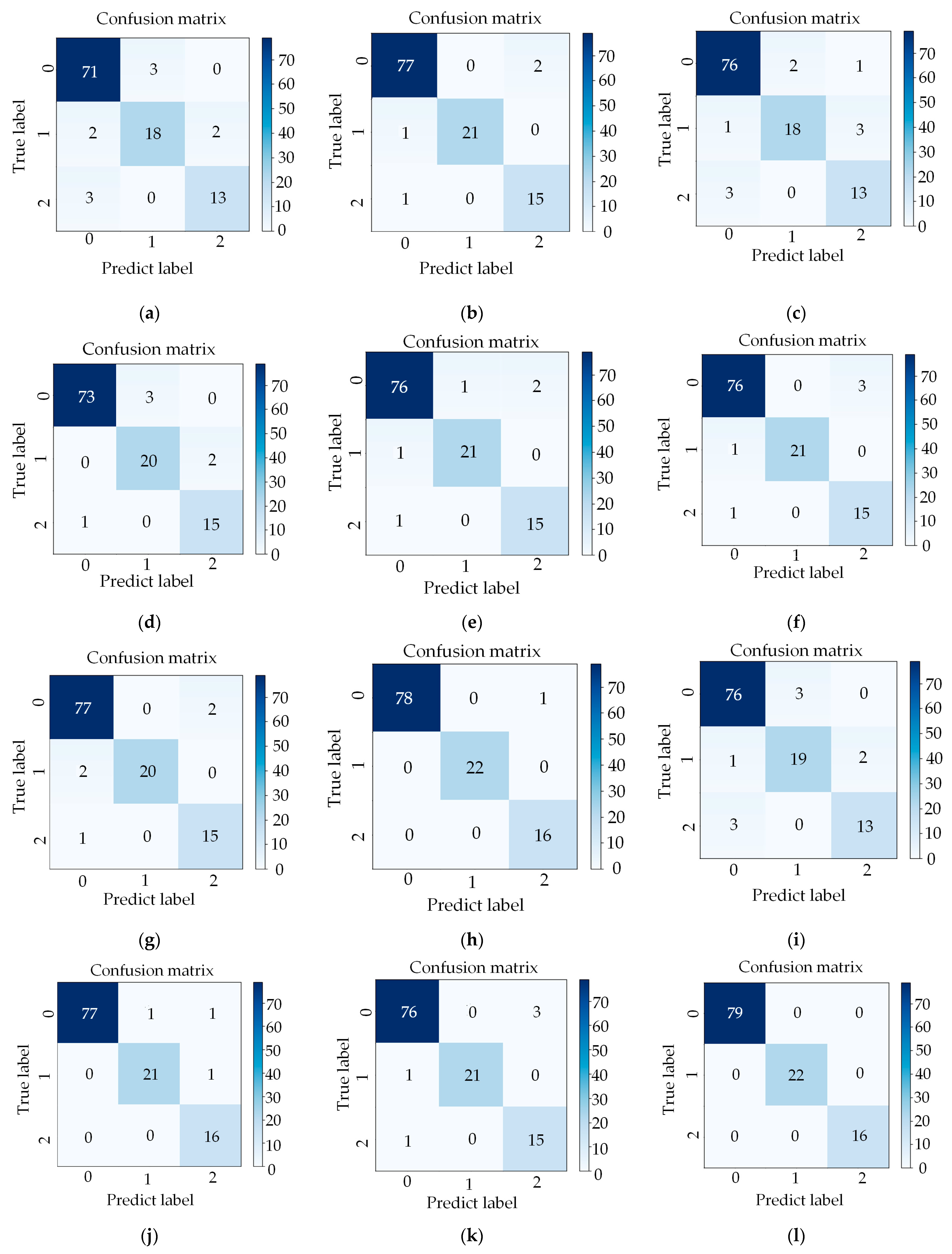
3.5. Algorithm Comparison
4. Conclusions
- (1)
- The accuracies of the different classification algorithms follow independent distributions with large variations, and the proposed MOA fault identification method, which combines environmental temperature and humidity interference suppression with an SAE, has an average accuracy of 99.7%.
- (2)
- The average accuracy of the fault recognition algorithm based on an SAE increased by 1.2%, 0.6%, and 0.9% compared to the values for the fault recognition algorithms based on SVM, RF, and LR, respectively.
- (3)
- Compared to traditional MOA fault recognition algorithms only considering the resistive current, the average accuracy of the MOA fault recognition algorithm with multi-feature fusion of the resistive current, environmental temperature, and humidity increased by 2%, and the proposed MOA fault recognition algorithm suppressing the interference of environmental temperature and humidity on resistive current increased by 3.7%.
Author Contributions
Funding
Data Availability Statement
Conflicts of Interest
Nomenclature
| Ir | Resistive current |
| Ir0 | Truth value of resistive current |
| Ir’ | Corrected value of resistive current |
| ΔIr | Difference between truth value and corrected value of resistive current |
| b | Fitting coefficient |
| t | Temperature |
| h | Relative humidity |
| N | Number of data samples |
| K | Maximum number of iterations |
| k | Number of iterations at termination |
| ɛ | Threshold of iterative convergence |
| u | Standardized residual indicator |
| q | Weight value |
| G | Fitting surface |
| W1 | Encoder weight |
| W2 | Decoder weight |
| a1 | Encoder offset |
| a2 | Decoder offset |
| x1 | Input vector of SAE |
| x2 | Feature parameter obtained from the first encoder |
| x3 | Feature parameter obtained from the second encoder |
| y1 | Feature parameter obtained from the first decoder |
| fe | Activate function of encoder |
| fd | Activate function of decoder |
| ρ | Pearson correlation coefficient |
| E | Mathematical expectation |
| A | Variable to be analyzed |
| B | Variable to be analyzed |
| H | Kruskal–Wallis test coefficient |
| n | Value of samples |
| M | Number of samples |
| R | Sum of the rank of all the samples |
| C | Sum of the value of samples |
References
- Ranjbar, B.; Darvishi, A.; Dashti, R.; Shaker, H.R. A survey of diagnostic and condition monitoring of metal oxide surge arrester in the power distribution network. Energies 2022, 15, 8091. [Google Scholar] [CrossRef]
- Christodoulou, C.A.; Vita, V.; Mladenov, V.; Ekonomou, L. On the computation of the voltage distribution along the non-linear resistor of gapless metal oxide surge arresters. Energies 2018, 11, 3046. [Google Scholar] [CrossRef]
- Christodoulou, C.A.; Ekonomou, L.; Fotis, G.P.; Gonos, I.F.; Sathopulos, I.A. Assessment of surge arrester failure rate and application studies in Hellenic high voltage transmission lines. Electr. Power Syst. Res. 2010, 80, 176–183. [Google Scholar] [CrossRef]
- Chen, Y.; Shu, S.; Wu, H.; Wang, G.; Chen, C. Inverse distance weighted improved KNN algorithm for defect diagnosis of MOA. J. Fuzhou Univ. (Nat. Sci. Ed.) 2022, 50, 635–641. [Google Scholar]
- Ma, Z.; Ruan, J.; Gan, Y.; Zhang, C.; Wang, J.; Du, Z. Research on resistive current calculation method of MOA based on RC network. High Volt. Appar. 2019, 55, 47–53+61. [Google Scholar]
- Luo, T.; Hu, W.; Liu, K. On-line measurement of metal oxide surge arrester based on harmonic analysis method. Electr. Switchg. 2011, 49, 34–36. [Google Scholar]
- Zhang, J. Application of infrared temperature measurement technology to live detection of zinc oxide arrester. High Volt. Appar. 2015, 51, 200–204. [Google Scholar]
- Liu, H.; Li, H.; Cao, Z.; Ding, Z.; Zhao, X. Arrester fault diagnosis based on resistive current detection and infrared thermal imaging technology. Insul. Surge Arresters 2016, 139, 75–78. [Google Scholar]
- Wei, S.; Deng, W.; Lei, H.; Mao, W.; Shi, Z.; Liu, W. Study on fault simulation and defect detection of 500 kV MOA. Insul. Surge Arresters 2019, 142, 109–114. [Google Scholar]
- Cao, H.; Yang, Z.; Hua, R.; Yang, H.; Ren, J. Study on algorithm of resistive current of MOA. High Volt. Appar. 2015, 51, 32–36. [Google Scholar]
- Dobrić, G.; Žarković, M. Fuzzy expert system for metal-oxide surge arrester condition monitoring. Electr. Eng. 2021, 103, 91–101. [Google Scholar] [CrossRef]
- Zhou, A.; Song, H.; Fang, Y.; Chang, Z. Fault diagnosis of MOVA based on evidence theory. Appl. Mech. Mater. 2014, 556, 2685–2688. [Google Scholar] [CrossRef]
- Huang, S.; Hsieh, C.H. A method to enhance the predictive maintenance of ZnO arresters in energy systems. Int. J. Electr. Power Energy Syst. 2014, 62, 183–188. [Google Scholar] [CrossRef]
- Bassi, W.; Tatizawa, H. Early prediction of surge arrester failures by dielectric characterization. IEEE Electr. Insul. Mag. 2016, 32, 35–42. [Google Scholar] [CrossRef]
- Wei, D.; Jiang, Y.; Zhang, X.; Li, L.; Wei, Z.; Xue, F.; Li, H.; Xie, J. Comprehensive evaluation method of operation status of zinc oxide surge arrester based on information fusion. Insul. Surge Arresters 2019, 142, 68–74. [Google Scholar]
- Zhao, Y.; Wang, Y.; Qin, P.; Zhang, J.; Li, M. Study on state evaluation of zinc oxide arrester based on fuzzy set pair analysis. Electr. Electron. 2020, 40, 28–31. [Google Scholar]
- Li, T.; Fang, W. Research on calculation method of resistive current of metal oxide arrester based on particle swarm optimization. Electr. Eng. 2021, 22, 104–108. [Google Scholar]
- Yang, Z.; Cao, H.; Li, P.; Cheng, Z.; Zhu, J. On-line monitoring of metal oxide arrester using genetic algorithm. High Volt. Eng. 2015, 41, 3104–3109. [Google Scholar]
- Lira, G.R.S.; Costa, E.G. MOSA monitoring technique based on analysis of total leakage current. IEEE Trans. Power Deliv. 2013, 28, 1057–1062. [Google Scholar] [CrossRef]
- Lira, G.R.S.; Costa, E.G.; Ferreira, T.V. Metal-oxide surge arrester monitoring and diagnosis by self-organizing maps. Electr. Power Syst. Res. 2014, 108, 315–321. [Google Scholar] [CrossRef]
- Hoang, T.T.; Cho, M.Y.; Alam, M.N.; Vu, Q.T. A novel differential particle swarm optimization for parameter selection of support vector machines for monitoring metal-oxide surge arrester conditions. Swarm Evol. Comput. 2018, 38, 120–126. [Google Scholar] [CrossRef]
- Khodsuz, M.; Mirzaie, M. Monitoring and identification of metal–oxide surge arrester conditions using multi-layer support vector machine. IET Gener. Transm. Distrib. 2015, 9, 2501–2508. [Google Scholar] [CrossRef]
- Chen, C.N.; Hoang, T.T.; Cho, M.Y. Parameter optimisation of support vector machine using mutant particle swarm optimisation for diagnosis of metal-oxide surge arrester conditions. J. Exp. Theor. Artif. Intell. 2019, 31, 163–175. [Google Scholar] [CrossRef]
- Wei, B.; Zuo, Y.; Liu, Y.; Luo, W.; Wen, K.; Deng, F. Novel MOA fault detection technology based on small sample infrared image. Electronics 2021, 10, 1748. [Google Scholar] [CrossRef]
- Zhang, C.; Guo, Y.; Li, M. Review of development and application of artificial neural network models. Comput. Eng. Appl. 2021, 57, 57–69. [Google Scholar]
- Ding, S.; Li, H.; Su, C.; Yu, J.; Jin, F. Evolutionary artificial neural networks: A review. Artif. Intell. Rev. 2013, 39, 251–260. [Google Scholar] [CrossRef]
- Zhou, N.; Liao, J.; Wang, Q.; Li, C.; Li, J. Analysis and prospect of deep learning application in smart grid. Autom. Electr. Power Syst. 2019, 43, 180–191. [Google Scholar]
- Zhang, Z.; Zhang, D.; Qiu, R. Deep reinforcement learning for power system applications: An overview. CSEE J. Power Energy Syst. 2019, 6, 213–225. [Google Scholar]
- Ruan, Y.; Ye, X.; Deng, M.; Wang, X.; Yang, L.; Shu, Q. A new online monitoring method for MOA based on A-VMD and ASVD. Electric Power 2021, 54, 177–185. [Google Scholar]
- Tuczek, M.N.; Bröker, M.; Hinrichsen, V.; Göhler, R. Effects of continuous operating voltage stress and AC energy injection on current sharing among parallel-connected metal–oxide resistor columns in arrester banks. IEEE Trans. Power Deliv. 2015, 30, 1331–1337. [Google Scholar] [CrossRef]
- Yang, Z.; Chen, L.; Du, Z.; Sun, Y. Application on capacitance during the degradation of ZnO varistor. High Volt. Eng. 2010, 36, 2167–2172. [Google Scholar]
- Huang, X.; Luo, B.; Wang, Y.; Li, X. Influence of climatic factors on on-line monitoring of MOA using grey relational analysis. High Volt. Eng. 2010, 36, 1468–1474. [Google Scholar]
- Seyyedbarzegar, S.M.; Mirzaie, M.; Khodsuz, M. A new approach to electrical modeling of surge arrester considering temperature effect on VI characteristic. Measurement 2017, 111, 295–306. [Google Scholar] [CrossRef]
- Xiao, S. Practicality of Online Monitoring of Substation Surge Arrester and Influence Factors of the Research and Analysis. Master’s Thesis, Fuzhou University, Fuzhou, China, 2017. [Google Scholar]
- Ding, G.; Lu, F.; Liu, Y.; Xing, L. Research of mathematical morphology in restraining interference in on-site monitoring of metal oxide surge arrester. High Volt. Eng. 2006, 32, 44–46. [Google Scholar]
- Wang, Z. Lightning Arrester Online Monitoring System in Inner Mongolia Power Grid Operation Analysis. Master’s Thesis, North China Electric Power University, Beijing, China, 2015. [Google Scholar]
- Xu, T.; Qin, S.; Mei, G.; Zhang, B.; Li, R.; Zhang, Y. On-line monitoring and evaluation of EHV composite insulators based on leakage currents and environmental conditions. Insul. Surge Arresters 2014, 137, 6–15. [Google Scholar]
- Zhao, D.; Xiao, R.; Si, W.; Han, Z.; Zhang, J.; Zhou, Y.; Guo, J. Influence of temperature on characteristic parameters of metal oxide surge arrester (MOA) and discussion on correction method. Insul. Surge Arresters 2018, 141, 82–87. [Google Scholar]
- Li, H.; Liu, J.; Xu, B. The modified method of MOA on-line monitoring parameters by eliminating external environmental factors interference. High Volt. Eng. 2018, 44, 2580–2586. [Google Scholar]
- Shi, Y.; Xue, F.; Chen, X.; Yang, L. The influence of weather on full current measurement of 110 kV ZnO arrester. Insul. Surge Arresters 2023, 146, 43–51. [Google Scholar]


| Reality | Prediction | |
|---|---|---|
| Positive Class | Negative Class | |
| Positive class | TP | FN |
| Negative class | FP | TN |
| Correlation | No Correlation | Weak Correlation | Moderate Correlation | Strong Correlation | Extremely Strong Correlation |
|---|---|---|---|---|---|
| Numerical value | 0.0–0.2 | 0.2–0.4 | 0.4–0.6 | 0.6–0.8 | 0.8–1.0 |
| Ambient Temperature | Ambient Humidity | |
|---|---|---|
| Resistive current | 0.796960 | 0.434868 |
| Resistive current after temperature and humidity interference suppression | 0.026346 | 0.001883 |
| Sample 1 − Sample 2 | Inspection Statistics | Standard Test Statistics | Significance |
|---|---|---|---|
| SAE + ③ − SVM + ① | 444.98 | 12.83 | 0.00 |
| SAE + ③ − SVM + ② | 302.62 | 8.72 | 0.00 |
| SAE + ③ − SVM + ③ | 155.04 | 4.47 | 8.00 × 10⁻⁶ |
| SA E+ ③ − LR + ① | −441.02 | −12.72 | 0.00 |
| SAE + ③ − LR + ② | −217.62 | −6.27 | 3.45 × 10⁻¹⁰ |
| SAE + ③ − LR + ③ | −141.34 | −4.07 | 4.68 × 10⁻⁶ |
| SAE + ③ − RF + ① | −349.38 | −10.07 | 0.00 |
| SAE + ③ − RF + ② | −299.44 | −8.63 | 0.00 |
| SAE + ③ − RF + ③ | −264.08 | −7.61 | 2.59 × 10⁻¹⁴ |
| SAE + ③ − SAE + ① | −472.74 | −13.63 | 0.00 |
| SAE + ③ − SAE + ② | −48.30 | −1.39 | 0.04 |
| Algorithm | Method | Recall Rate | Precision | F1-Score | Accuracy | Computation Time (s) |
|---|---|---|---|---|---|---|
| SVM | ① | 0.95783 | 0.95627 | 0.95705 | 0.95641 | 0.28492 |
| ② | 0.96832 | 0.96511 | 0.96671 | 0.96902 | 3.65214 | |
| ③ | 0.98101 | 0.98284 | 0.98192 | 0.98182 | 0.65291 | |
| RF | ① | 0.96526 | 0.96731 | 0.96629 | 0.96533 | 0.30492 |
| ② | 0.96101 | 0.96563 | 0.96331 | 0.96926 | 2.98562 | |
| ③ | 0.97181 | 0.97166 | 0.97173 | 0.97215 | 0.59254 | |
| LR | ① | 0.95818 | 0.95861 | 0.95991 | 0.95588 | 0.21456 |
| ② | 0.97209 | 0.97558 | 0.97383 | 0.97629 | 3.98756 | |
| ③ | 0.98187 | 0.98421 | 0.98304 | 0.98295 | 0.62135 | |
| SAE | ① | 0.94048 | 0.93103 | 0.93573 | 0.95181 | 0.31892 |
| ② | 0.98532 | 0.99101 | 0.98815 | 0.99209 | 5.53882 | |
| ③ | 0.99856 | 0.98621 | 0.99234 | 0.99709 | 0.52849 |
Disclaimer/Publisher’s Note: The statements, opinions and data contained in all publications are solely those of the individual author(s) and contributor(s) and not of MDPI and/or the editor(s). MDPI and/or the editor(s) disclaim responsibility for any injury to people or property resulting from any ideas, methods, instructions or products referred to in the content. |
© 2023 by the authors. Licensee MDPI, Basel, Switzerland. This article is an open access article distributed under the terms and conditions of the Creative Commons Attribution (CC BY) license (https://creativecommons.org/licenses/by/4.0/).
Share and Cite
Shu, S.; Zhang, X.; Wang, G.; Zeng, J.; Ruan, Y. A Fault Identification Method for Metal Oxide Arresters Combining Suppression of Environmental Temperature and Humidity Interference with a Stacked Autoencoder. Energies 2023, 16, 8033. https://doi.org/10.3390/en16248033
Shu S, Zhang X, Wang G, Zeng J, Ruan Y. A Fault Identification Method for Metal Oxide Arresters Combining Suppression of Environmental Temperature and Humidity Interference with a Stacked Autoencoder. Energies. 2023; 16(24):8033. https://doi.org/10.3390/en16248033
Chicago/Turabian StyleShu, Shengwen, Xiaoyao Zhang, Guobin Wang, Jinglan Zeng, and Ying Ruan. 2023. "A Fault Identification Method for Metal Oxide Arresters Combining Suppression of Environmental Temperature and Humidity Interference with a Stacked Autoencoder" Energies 16, no. 24: 8033. https://doi.org/10.3390/en16248033