Article

Two-Dimensional Geothermal Model of the Peruvian Andes above the Nazca Ridge Subduction

1
Dipartimento di Scienze Pure e Applicate (DiSPeA), Università di Urbino “Carlo Bo”, Via Aurelio Saffi, 2, 61029 Urbino, Italy
2
Scuola di Scienze e Tecnologie, Sezione di Geologia, Università degli Studi di Camerino, Via Gentile III da Varano, 7, 62032 Camerino, Italy
3
Istituto Nazionale di Geofisica e Vulcanologia, Via di Vigna Murata, 605, 00143 Rome, Italy
4
Department of Geosciences, University of Fribourg, 1700 Fribourg, Switzerland
*
Author to whom correspondence should be addressed.
Energies 2023, 16(23), 7697; https://doi.org/10.3390/en16237697
Submission received: 19 October 2023 / Revised: 13 November 2023 / Accepted: 17 November 2023 / Published: 21 November 2023
(This article belongs to the Collection Renewable Energy and Energy Storage Systems)

Abstract

:
The aseismic Nazca Ridge produces localized flat-slab subduction beneath the South American margin at latitudes 10° to 15° S. The geological evolution and the spatio-temporal pattern of deformation of the upper plate have been strongly influenced by the presence of the flat slab. In this study, we investigated the lithospheric thermal structure of this region by elaborating a 2D geothermal model along a section across the top of the Nazca Ridge, the Peru–Chile trench, the Andean Cordillera, and the Amazonian Basin, for a total length of 1000 km. For the sake of modelling, the crust of the overriding plate was subdivided into two parts, i.e., a sedimentary cover (including the entire lithostratigraphic sequence) and a crystalline basement. Applying an analytical methodology, we calculated geotherms and isotherms by setting (i) thickness, (ii) density, (iii) heat production, and (iv) thermal conductivity for each geological unit and considering (v) heat flux at the Moho, (vi) frictional heating produced by faults, and (vii) plate convergence rate. The resulting model could make a significant advance in our understanding of how flat slab geometry associated with the Nazca Ridge subduction affects the thermal structure and hence the tectonic evolution of the region.

1. Introduction

Understanding the thermal structure of the overriding plate of subduction systems is a fundamental issue for a series of applications, including the sustainable exploitation of geothermal energy, the identification of significant ore deposits, and the analysis of seismic hazard, besides providing more general constraints to the study of geodynamic processes. For this paper, we carried out this kind of study in a relevant sector of the South American Plate and Andean subduction system, at the locus of the Nazca Ridge subduction.
The Nazca Ridge is an aseismic ridge subducting beneath the South American Plate. It represents a thickened portion of the oceanic crust, showing an overall crustal thickness of 18 ± 3 km with a width of 200 km [1]. The subduction of the Nazca Ridge began approximately 11.2 million years ago at 11° S, with a trend of about N42° E. The subduction margin migrated progressively southward to the present collision zone around 4–5 Ma [2,3,4]. The presence of the thickened subducting Nazca Ridge triggered a localized flat-slab subduction phenomenon beneath the South American continental margin, particularly within the latitudinal range from 10° to 15° S. This peculiar geological setting exerts a strong influence on the kinematics and dynamics within the upper tectonic plate. The correlation between flat slabs and subducting ridges has been widely investigated and documented [5,6,7,8,9,10]. The presence of anomalously thick oceanic crust produces buoyancy that largely controls subduction dynamics [7]. Moreover, the presence of subducting aseismic ridges results in reduced extension of the overriding plate. This phenomenon can also induce localized shortening in the forearc region, proportional to the dimensions of the aseismic ridges [10]. Flat subduction significantly impacts stress distribution within the overriding plate, influencing the spatial distribution of seismicity in the upper plate [11]. Furthermore, in these geodynamic conditions, the asthenospheric wedge withdraws from the trench, with significant implications for the thermal structure of the upper plate [7]. In any case, the effects of the subduction of the Nazca Ridge on the Peruvian forearc system and on the development of the Andean Cordillera are still being investigated and are a topic of extensive debate. Thus, to attain a more exhaustive comprehension of the complex tectonic dynamics related to this specific sector of the Andean orogen, it is crucial to acknowledge the key role played by the rheological properties of the Earth’s crust and lithosphere, which are strongly associated with the thermal conditions. Notably, temperature is a significant factor affecting crustal viscosity, underscoring the need for a comprehensive investigation into the thermal structure present in our study area. The primary aim of this research is to focus on a detailed investigation of the lithospheric thermal structure of the upper plate above the Nazca Ridge, carried out through the development of a rigorous 2D geothermal model. This model extends across a transect of about 1000 km in length, oriented N48° E, that ranges from 10° S to 16° S, comprising all the main geological features of the area: the Peru–Chile trench, the Peruvian forearc system (West Pisco Basin and East Pisco Basin), and the entirety of the Andean Cordillera. The entire area has been thoroughly delineated within a comprehensive geological structural model, including both surface geology and all the deeper structures down to a total depth of 130 km, in order to provide a framework of the whole lithosphere. The crustal section has served as the starting point for the development of the thermal model. The analytical approach, which served as the basis for our investigation into surface heat flow and isotherm patterns, was formulated by Dragoni et al. [12]. The procedure has already been applied and validated in several geographical regions in recent years by Basilici et al. [13] and Santini et al. [14,15], and the results of these studies ensure its suitability and relevance for our specific research objectives. To obtain the most accurate results, the methodology has been specifically modified and adjusted for the study area through a meticulous analysis of the geological features. In order to create a concise and precise representation suitable for our model, we divided the overriding plate into three main layers. Each of these layers was characterized by fundamental geological parameters, including (i) thickness, (ii) density, (iii) heat production, and (iv) thermal conductivity. This division allowed us to capture the key geological variations within the overriding plate. Additionally, our model also includes (v) heat flux at the Moho, (vi) frictional heating produced by faults, and (vii) plate convergence rate. These factors were incorporated into the model to explore the geodynamics of the plates and their influence on heat distribution and fault behaviour within the region. We subsequently performed a comparative analysis, cross-referencing our results with previously published research and measured heat flux data from adjacent regions, specifically referring to Uyeda et al. [16], Henry and Pollack [17], and Molnar and England [18]. By integrating these geological parameters and dynamic variables, our model provides a comprehensive and accurate representation of the complex geological and thermal structure of the overriding plate. It serves as a key instrument within our scientific inquiry, allowing us to examine the relationship between the geometric characteristics of the flat slab related to the Nazca Ridge subduction process and its implications on the thermal regime within the region. Through the integration of various geological and geophysical parameters, our study aims to make a substantial contribution to the ongoing advancement of scientific knowledge relating to the complex tectonic evolution of the Peruvian Andean Cordillera.

2. Geological Background

The Andean orogen is a model of a continental mountain belt produced by subcontinental subduction, where the oceanic slab subducts beneath the continental plate [19]. The setting and geometry of the Andes vary substantially along their longitude. The largest sector is formed by the Central Andes; it ranges from 5°300′ S to 37° S and is, in turn, subdivided into three subsectors: Northern Central Andes, Central Andes Orocline, and Southern Central Andes [20]. The portion of the Andean Cordillera within Peruvian territory falls within the Northern Central Andes subsector and the northern part of the Central Andes Orocline subsector. The inner and older portion of the Peruvian Andes consists of Precambrian high-grade metamorphic basement including gneisses, amphibolites, and marbles. These rocks are covered by Paleozoic marine sediments and clearly outcrop only in the Eastern Cordillera. From the Middle Ordovician to the Upper Devonian, almost uninterrupted sedimentation events occurred, and the settled strata experienced significant deformation during the Hercynian orogenic phase, which occurred straddling the Late Devonian and Early Mississippian [21]. A transitional period began between the Late Permian and Early Triassic between the Hercynian geological orogenic phase and the onset of the Andean orogenic cycle, persisting until the present day [21]. Several structures developed within the Precambrian and Hercynian orogeny were inherited and reactivated during the Andean orogeny. The present-day features of the Peruvian Andes are predominantly linked to the Cenozoic tectonic evolution, with an alternation of sedimentation and tectogenic periods linked to the subduction dynamics. The Andean orogenic cycle can be divided into two distinct phases: a prolonged period of relative tectonic stability covering a period of time from the Triassic to the Late Cretaceous, and a shorter orogenic period characterized by five major phases of compressive deformation: the (i) Peruvian (Late Cretaceous), (ii) Incaic (Middle to Late Eocene), (iii) Quechua 1 (Lower Miocene), (iv) Quechua 2 (Tortonian), and (v) Quechua 3 (Messinian) phases [21]. These deformation phases occurred associated and sometimes alternated with episodes of volcanism of different and variable chemistry, sedimentation, and the settling of batholiths due to plutonic activity [21]. During the Peruvian phase, the first pervasive deformation episode occurred. During this phase, the Western and Eastern Peruvian troughs were uplifted, establishing the bases for the current Andean conformation. During the following phases, the fold and thrust belt developed during the Peruvian and Incaic ages was reactivated by the Quechua 1, Quechua 2, and Quechua 3 phases, producing a progressive migration of the deformation toward the foreland. By the Miocene era, the Andes Mountain Range was already established, with the Subandean Zone being incorporated later [21].
The area investigated in this study (Figure 1) is located around the transition from the Northern Central Andes to the Central Andes Orocline at the Nazca Ridge subduction zone. The area comprises (i) the Peruvian forearc system, subdivided into East and West Pisco basins [22]; (ii) the Western Cordillera, consisting of a western part with sequence stratigraphy dominated by the Coastal Batholiths [23] and an eastern part characterized by the Marañón fold and thrust belt; (iii) the Eastern Cordillera, an anticline structure characterized by tectonic shortening propagated during the Oligocene–Miocene tectonic inversion of the original Triassic–Jurassic rift system [20,24]; (iv) the Subandean Zone, including Camisea and Ene basins; and (v) the Fitzcarrald arch, an area overhead ~500 m above the adjacent basin [25], that marks the transition between the northern and southern parts of the Amazonian foreland basin [26].

3. Materials and Methods

The thermal structure investigation was based on a specific analytical procedure applied to a crustal model of the Nazca Ridge subduction region.

3.1. Lithospheric Model

The model consists of a section with a length of 1000 km trending 48° N. The section is aligned to the Nazca Ridge axis and runs from the top of the Nazca Ridge in the west to the Amazonian Basin in the east, progressively crossing the Peru–Chile trench, the forearc, and the Andean Cordillera (Figure 2). The cross-section reaches a depth of 130 km, aiming to intercept the upper plate Moho and lithospheric mantle, as well as the underlying subducting slab. Data on the Moho and slab geometry in this area were obtained from previously published models [27,28,29,30,31]. The profile obtained was compared and validated using the results from [3,8,32]. To process the model, the Move software from Petroleum Express was employed. Data on the seismicity of the area were obtained from the USGS catalog [33]. We considered all earthquakes that occurred in the last 50 years with Mw ≥ 6 in an area of 100 km around the cross-section (Figure 3). Focal mechanisms for these earthquakes were projected onto the vertical plane of the cross-section. To perform an accurate projection, we applied a double rotation procedure using the FaultKin software v8.1.2 (Allmendinger). In the first step, focal mechanisms were rotated along the vertical axis according to the strike value of the cross-section to align them. Subsequently, they were rotated along the horizontal axis to obtain a section view of the focal mechanism. Once this process was completed, the nodal plane of the focal mechanism perfectly coincided with the reactivated fault plane. After the focal mechanism was properly oriented, it was projected onto the section using the strike value of the nodal plane corresponding to the fault. Earthquake hypocentral distribution is consistent with most large thrust earthquakes being related to the subducting slab and therefore defining the subduction interface. Normal fault earthquakes also occur within the slab. The lithospheric model (Figure 4) was implemented with the necessary information to support the analytical procedure. For the shallowest part of the section, we used geological data and maps freely available on the INGEMMET website. Since there are no freely available geophysical data for this area, the geological section was constructed considering previously published geological sections of adjacent areas [34,35]. For simplification, we considered the whole lithosphere as composed of three main geological units: crystalline basement (B), Cenozoic–Mesozoic sedimentary cover (SC_1), and Paleozoic sedimentary cover (SC_2). For each unit, we estimated a set of parameters, including thickness, density, radiogenic heat production (RHP), and thermal conductivity. To prevent the heterogeneity of the sedimentary succession from causing errors in the model, we calculated the areal percentage and the thickness of each geological formation present in a buffer of 40 km around the section. We reclassified all the geological formations into lithological groups and assigned to each one a mean value of RHP according to Vila et al. [36]. Then, we calculated an average of the RHP values weighted for both the areal percentage and the thickness of each lithological group. In this way, we obtained weighted average values of the RHP for SC_1 and SC_2. In the cross-section, we set 11 pseudo-wells in which we performed the modelling.

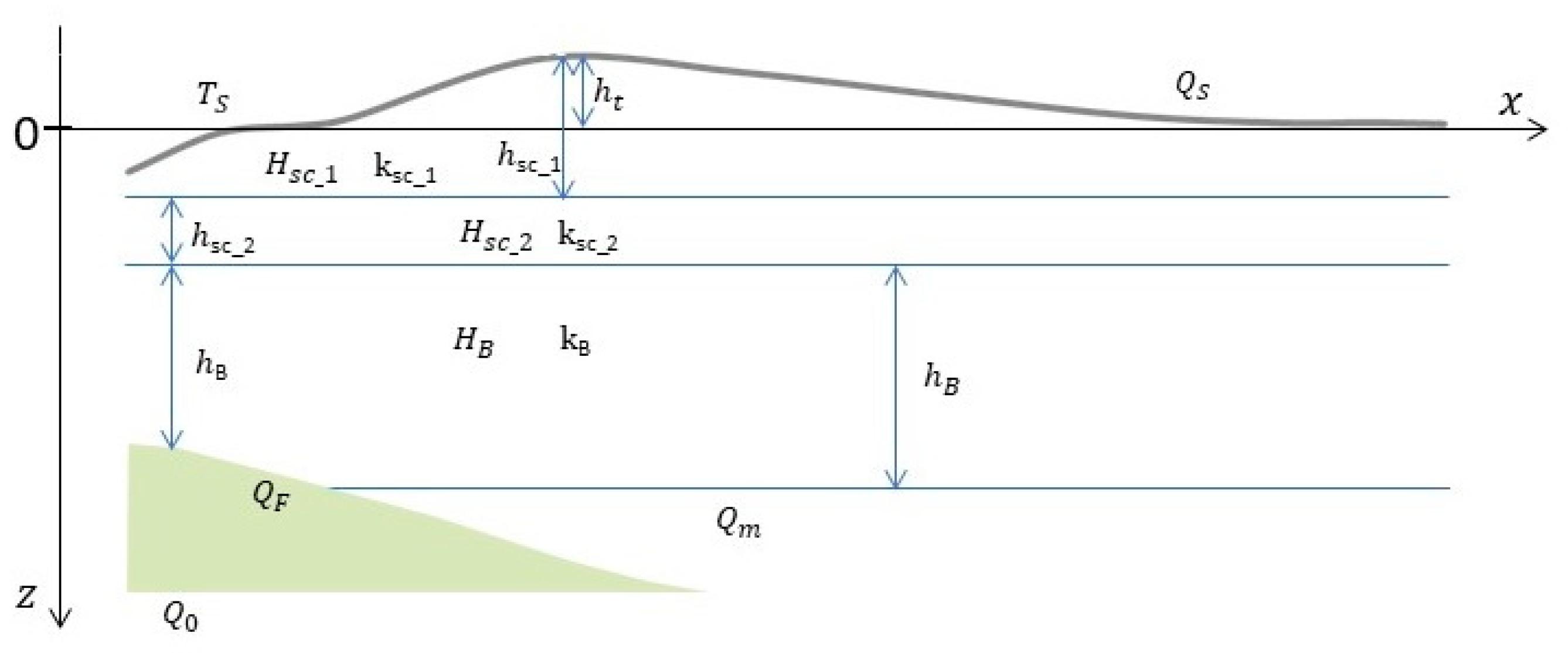
3.2. Thermal Modelling

To obtain the surface heat flow and the isotherms, we used the analytical procedure developed by Dragoni et al. [12], which was verified in different geographic zones in recent years by Basilici et al. [13] and Santini et al. [14,15], specifically modified for the area of study. The mathematical representation of the thermal model presented below consists of three layers of variable thickness, over a half-space (Figure 5). The mean sea level (m.s.l.) is at z = 0, with z positive downward. The unidimensional calculation procedure was applied to each of the 11 pseudo-wells located on the crustal model. The resulting heat flow was then interpolated using a sixth-order polynomial equation.
In the computation of the surface heat flow Q s , we considered (i) the contribution of the mantle heat flow Q m , (ii) the radiogenic heat, and (iii) the frictional heat Q F in the megathrust zone. We obtained the following equation:
Q s =   Q + H S C _ 1 h S C _ 1 + H S C _ 2 h S C _ 2 + H B D ( 1 e h B D )
where h S C _ 1 and H S C _ 1 are SC_1 thickness and heat productivity, h S C _ 2 and H S C _ 2 are SC_2 thickness and heat productivity,   h B and H B are basement thickness and heat productivity, and D is the depth scale. For PW_1, across the accretionary wedge, the parameter H S C was substituted by H S S (heat productivity for sandstone; Table 1).
In Equation (1), Q′ represents the heat flow at the base of the model due to the heat flow coming from the mantle and to the frictional heat of the thrust when it is present.
For the megathrust zone, we considered Q = ( Q 0 + Q F )   S 1 , where Q 0 is the oceanic mantle heat flow and S = 1 + b z f   v   s i n δ k , with b 1 , is the reducing divisor near the megathrust fault [18]. For the continental zone, we considered Q = Q m . Instead, H S C 1 h S C 1 and H S C _ 2 h S C _ 2 are the contributions of each sedimentary layer considering a constant radiogenic source [14,38,39], while the last term of Equation (1) is the contribution of the basement considering a radiogenic source with an exponential trend [12,40,41].
The temperature in the uppermost layer (thickness h S C _ 1 ) is controlled by (i) the heat flow at the top of SC_2, (ii) the contribution of the radiogenic source of this layer, and (iii) the surface temperature (Equation (2)). In the second layer (SC_2), the geotherm initial value is the temperature at the bottom of the first layer to which is added the temperature variation due to the radiogenic source within SC_2 and to the heat flow at its bottom (Equation (4)). Finally, the temperature in the basement depends on the mantle flow and on its own radiogenic source, to which is added the temperature variation due to the radiogenic source within SC_1 and SC_2. In addition, only in the megathrust zone, the frictional heat contribution is considered in the three layers.
The temperature in the first layer (thickness h S C _ 1 ) is:
T z = T S + T S C _ 1 H z ,       z t z z t + h S C _ 1
and the depth-dependent term T S C _ 1 H is defined as:
T S C _ 1 H ( z ) = Q s k S C _ 1 ( z z t ) H S C _ 1 2 k S C _ 1 ( z z t ) 2
where k S C _ 1 and H S C _ 1 are SC_1 thermal conductivity and heat productivity.
In the second layer (thickness h S C _ 2 ), we obtain:
T z = T S + T S C _ 1 H h S C _ 1 + T S C _ 2 H z ,   z t + h S C _ 1 < z z t + h S C _ 1 + h S C _ 2
defining the depth-dependent term T S C _ 2 H as:
T S C _ 2 H z = Q s H S C _ 1 h S C _ 1 k S C _ 2 z z t h S C _ 1 H S C _ 2 2 k S C _ 2 ( z z t h S C _ 1 ) 2
where k S C _ 2 and H S C _ 2 are SC_2 thermal conductivity and heat productivity.
Finally, in the basement (thickness h B ), we obtain:
T z = T S + T S C _ 1 H h S C _ 1 + T S C _ 2 H h S C _ 2 + T B H z , z t + h S C _ 1 + h S C _ 2 < z z t + h S C _ 1 + h S C _ 2 + h B
defining the depth-dependent term T B H as:
T B H z = Q   k B z z t h S C _ 1 h S C _ 2 + H B D 2 k B 1   e z z t h S C _ 1 h S C _ 2 D
where k B and H B are basement thermal conductivity and heat productivity and D is the depth scale.
The terms used in the equations are defined in Table 2.
Table 2. Data considered in the model and parameters included in the equations [36,42,43,44,45,46,47].
z t (m)Ground elevation (negative) or sea depth (positive) related to m.s.l.
h S C _ 1 (m)Sedimentary cover (Cenozoic-Mesozoic) thickness
h S C _ 2 (m)Sedimentary cover (Paleozoic) thickness
h B (m)Basement thickness
H S C _ 1 = 0.83   µ W m 3 RHP * of sedimentary cover (Cenozoic-Mesozoic)[36]
H S C _ 2 = 1.2   µ W m 3 RHP * of sedimentary cover (Paleozoic)[36]
H B = 1.6   µ W m 3 RHP * of basement thickness[36]
k S C _ 1 = 2.1   W m 1 K 1 Thermal conductivity of sedimentary cover (Cenozoic-Mesozoic)[42]
k S C _ 2 = 2.4   W m 1 K 1 Thermal conductivity of sedimentary cover (Paleozoic)[42]
k B = 2.7   W m 1 K 1 Thermal conductivity of the basement[42]
κ = 10 6   m 2 s 1 Thermal diffusivity[43]
µ = 0.7 Coefficient of static friction[43]
ρ S C _ 1 = 2.4 10 3 k g   m 3 Density of sedimentary cover (Cenozoic-Mesozoic)[44]
ρ S C _ 2 = 2.4 10 3 k g   m 3 Density of sedimentary cover (Paleozoic)[44]
ρ B = 2.85 10 3 k g   m 3 Density of the basement[44]
D = 10   k m Depth scale[45]
x f   ( k m ) Horizontal coordinate for points on the megathrust fault
z f   ( k m ) Vertical coordinate for points on the megathrust fault
δ = a r c t g z f x f Dip angle of the megathrust fault
λ = 0.96 Pore fluid factor[46]
v = 7.7 c m a 1 Relative plate velocity[46]
Q F = µ ρ g h 1 λ v Fritional heat flow density
Q o = 60   m W m 2 Oceanic heat flow density from the mantle[47]
Q m = 20   m W m 2 Continental heat flow density from the mantle[47]
Q s   ( m W m 2 ) Surface heat flow density
T S = 15   ° C Surface temperature
* Radiogenic Heat Productivity.

4. Results

With the aim of obtaining isotherms defining the thermal structure of the overriding plate, we computed the geotherm and the heat flow Q s for each pseudo-well along the cross-section (Figure 4). The resulting geotherm profiles (Figure 6) describe a well-defined correlation between temperature increase and depth. The geotherm profiles of PW_1 and PW_2 exhibit relatively lower temperatures compared to the other pseudo-wells. Notably, PW_1 is located in the accretionary wedge. Geotherms associated with PW_3, PW_4, and PW_7 are very close to each other and exhibit a consistent temperature–depth trend down to a depth of 25 km. Beyond this depth, PW_3 experiences a progressive increase in temperature, in contrast to PW_4 and PW_7, which maintain a consistent trend. PW_5 and PW_6 geotherms display a similar temperature–depth relationship, even if PW_5 shows the highest temperature. Finally, PW_8, PW_9, PW_10, and PW_11 are almost coincident: at shallower depths, their temperatures approximate the values of PW_3 and PW_4, but around 25 km, they tend to align with PW_6.
To constrain the isotherms near the megathrust, we estimated the temperature along the slab surface within a distance of 150 km from the subduction trench.
Figure 7 shows the computed surface heat flow Q s and the isotherms obtained by sixth-order polynomial interpolation. The results point out that the area within the megathrust zone exhibits the lowest heat flow values. As a matter of fact, from PW_1 to PW_4, values range from 25.57 to 39.14 mW/m2. Moving eastward, the surface heat flow tends to increase close to PW_5, reaching a maximum value of 45.77 mW/m2, and then remains almost constant around a mean value of 42 mW/m2. These relatively high values are strongly influenced by the radiogenic heat produced by the basement (HB). The isotherms show a trend that is roughly sub-parallel to the surface in the eastern part of the cross-section, whereas they rise to form a thermal dome centered in the Western Cordillera ca. 250 km NE of the subduction trench. The cool subducting slab induces a deepening of the isotherms, defining the southwestern limb of the thermal dome.

5. Discussion

Our model exhibits geotherms and surface heat flow Q s values computed at 11 points distributed along a transect of the Peruvian Andean Cordillera. These values were interpolated using a sixth-order polynomial equation in order to obtain a general trend of the surface heat flow for the whole area and a set of isotherms that define the thermal structure of the lithosphere above the Nazca Ridge subduction zone. Geotherms (Figure 6) display trends mostly comparable to each other. The greatest analogies are among PW_8, PW_9, PW_10, and PW_11, which are substantially coincident. Observing the location of these pseudo-wells along the cross-section, it is clear that the thickness of the basement at those points is almost constant. This relation also occurs in PW_3, PW_4, and PW_7, but in this instance, PW_3 at depths greater than 25 km shows a different trend, and this may be due to the fact that PW_3 is extremely close to the subduction interface. PW_5 and PW_6 show the highest temperatures, and in that position, the basement reaches the maximum thickness. In our assessment, this observed behaviour constitutes evidence of the significant impact exerted by radiogenic heat production of the basement on its contribution to the heat flow; we have also considered the contribution of the topography altimetry. The computed values of surface heat flow Q s range from a minimum of 25.57 mW/m2 to a maximum of 45.77 mW/m2. These values were cross-checked with previously published results. The megathrust zone, between PW_1 and PW_4, shows the lowest values (from 25.57 to 39.14 mW/m2), in good agreement with the values calculated by Molnar and England [18] that pointed out an average value of 33 ± 5 mW/m2 for the offshore zone of Peru. Nevertheless, observed values from Uyeda et al. [16] and Henry and Pollack [17] and their related error bars were projected onto the computed model. The location of the observed points is shown in Figure 1. At a regional scale, the obtained analytical curve is consistent with the observed surface heat flux Q s values. The surface heat flow Q s value of 45.77 mW/m2 in the area of PW_5 agrees with the value of 44 mW/m2 observed by Henry and Pollack [17] for the sites of Marcahui (obs_5) and Cerro Verde (obs_7) in the south-eastern onshore zone of Peru. Moreover, the surface heat flow value computed in PW_7 (38.16 mW/m2) is consistent with the values observed by the same authors for the site of La Granja (obs_4). However, for a meaningful comparison of observed values with the theoretical curve, the distribution of the measurement sites from the cross-section trace must be considered. Indeed, distances of the sites from the cross-section range from 200 km to 900 km, implying large variations in geological and geodynamic settings. Moreover, we must also consider the uncertainty that affects the observed data, ranging from 10% to 20%, as pointed out by Uyeda et al. [19] and Henry and Pollack [17]. So, we can assume that at a regional scale, the trend of the computed values is consistent with the observed values, and the mismatch may be ascribed to the influence of local geological conditions and to the error in measurement. Computed isotherms describe a thermal dome below the Western Cordillera, between PW_4 and PW_6. In that area, the Moho tends to become deeper, and the basement is thicker than in the surrounding areas. So, the computed thermal structure seems to be in contrast with the geological setting. Taking into consideration the constraints under which the structural model has been set up [3,8,27,28,29,30,31,32,34,35] and the relationship between the surface heat flow Q s values observed [16,17,18] and the ones computed using the analytical procedure, we believe that the presence of the thermal dome may be linked to some density anomaly in the area. Indeed, in the analytical procedure, we consider the density of the basement as constant. In the area affected by the thermal dome, the basement is thickened, and, in this condition, it is likely that the mantle density at the deepest part is slightly higher than estimated. At this moment, we are not able to evaluate if this option is realistic and functional. We will additionally employ gravimetric techniques to conduct further validation and to thoroughly analyse the characteristics of the thermal dome.

6. Conclusions

The thermal model presented in this study aims to provide new insights into the tectonics of the Peruvian Andean Cordillera, which is strongly influenced by the presence of the subducting Nazca Ridge. Starting from a detailed crustal model and applying an analytical procedure that accounts for specific geological and geophysical parameters, we were able to thoroughly reconstruct the thermal structure of the upper plate above the Nazca Ridge subduction zone. Our results reveal that the surface heat flow Q s and the shape of isotherms are mainly influenced by (i) the presence of the megathrust and (ii) the thickness of the basement. In fact, the lithosphere closest to the trench, where subduction begins, has lower surface heat flux Q s values (from 25.57 to 39.14 mW/m2), while moving eastward, the surface heat flux Q s values tend to be higher and almost constant. The highest surface heat flux Q s values were observed in the areas where the basement has the greatest thickness. Furthermore, the computed surface heat flux Q s values resulting from this model are consistent with the values observed by Uyeda et al. [16] and Henry and Pollack [17], taking into account the error percentage associated with the measured values and, especially, the areal distribution of measurement points, which involve an extremely heterogeneous area from a geological and geodynamical perspective. The distribution of isotherms indicates the presence of a thermal dome below the western part of the Cordillera, where ideally the isotherms should follow the trend of the Moho. The nature of this dome will be further investigated using gravimetric modelling techniques.

Author Contributions

Conceptualization, S.C., S.M., A.M., M.B. and S.S.; methodology, S.C., S.M., A.M., M.B. and S.S.; software, A.M. and S.C.; validation, S.C., A.M., S.M. and S.S.; formal analysis, S.C., A.M. and S.S.; investigation, S.C., S.M., A.M. and S.S.; resources, S.C., A.M. and S.S.; data curation, A.M., S.C., S.M. and S.S.; writing—original draft preparation, S.C.; writing—review and editing, S.M.; visualization, S.C.; supervision, S.M. and S.S.; project administration, S.S.; funding acquisition, S.S. All authors have read and agreed to the published version of the manuscript.

Funding

This research received no external funding.

Data Availability Statement

Data are contained within the article.

Acknowledgments

The authors are grateful to the editor for his helpful support in organizing the manuscript and to three anonymous reviewers for helpful and constructive comments.

Conflicts of Interest

The authors declare no conflict of interest.

References

  1. Woods, M.T.; Okal, E.A. The structure of the Nazca ridge and Sala y Gomez seamount chain from the dispersion of Rayleigh waves. Geophys. J. Int. 1994, 117, 205–222. [Google Scholar] [CrossRef]
  2. Macharé, J.; Ortlieb, L. Plio-Quaternary vertical motions and the subduction of the Nazca Ridge, central coast of Peru. Tectonophysics 1992, 205, 97–108. [Google Scholar] [CrossRef]
  3. Hampel, A. The migration history of the Nazca Ridge along the Peruvian active margin: A re-evaluation. Earth Planet. Sci. Lett. 2002, 203, 665–679. [Google Scholar] [CrossRef]
  4. Zeumann, S.; Hampel, A. Deformation of erosive and accretive forearcs during subduction of migrating and non-migrating aseismic ridges: Results from 3-D finite element models and application to the Central American, Peruvian, and Ryukyu margins. Tectonics 2015, 34, 1769–1791. [Google Scholar] [CrossRef]
  5. Li, C.; Clark, A.L. Tectonic effects of the subducting Nazca Ridge on the southern Peru continental margin. Mar. Pet. Geol. 1994, 11, 575–586. [Google Scholar]
  6. Hagen, R.A.; Moberly, R. Tectonic effects of a subducting aseismic ridge: The subduction of the Nazca Ridge at the Peru Trench. Mar. Geophys. Res. 1994, 16, 145–161. [Google Scholar] [CrossRef]
  7. Gutscher, M.A. Andean subduction styles and their effect on thermal structure and interplate coupling. J. South Am. Earth Sci. 2002, 15, 3–10. [Google Scholar] [CrossRef]
  8. Hampel, A.; Kukowski, N.; Bialas, J.; Huebscher, C.; Heinbockel, R. Ridge subduction at an erosive margin: The collision zone of the Nazca Ridge in southern Peru. J. Geophys. Res. Solid Earth 2004, 109, B02101. [Google Scholar] [CrossRef]
  9. Antonijevic, S.K.; Wagner, L.S.; Kumar, A.; Beck, S.L.; Long, M.D.; Zandt, G.; Tavera, H.; Condori, C. The role of ridges in the formation and longevity of flat slabs. Nature 2015, 524, 212–215. [Google Scholar] [CrossRef]
  10. Flórez-Rodríguez, A.G.; Schellart, W.P.; Strak, V. Impact of aseismic ridges on subduction systems: Insights from analog modeling. J. Geophys. Res. Solid Earth 2019, 124, 5951–5969. [Google Scholar] [CrossRef]
  11. Kumar, A.; Wagner, L.S.; Beck, S.L.; Long, M.D.; Zandt, G.; Young, B.; Tavera, H.; Minaya, E. Seismicity and state of stress in the central and southern Peruvian flat slab. Earth Planet. Sci. Lett. 2016, 441, 71–80. [Google Scholar] [CrossRef]
  12. Dragoni, M.; Doglioni, C.; Mongelli, F.; Zito, G. Evaluation of Stresses in Two Geodynamically Different Areas: Stable Foreland and Extensional Backarc. Pure Appl. Geophys. 1996, 146, 319–341. [Google Scholar] [CrossRef]
  13. Basilici, M.; Mazzoli, S.; Megna, A.; Santini, S.; Tavani, S. 3-D Geothermal Model of the Lurestan Sector of the Zagros Thrust Belt, Iran. Energies 2020, 13, 2140. [Google Scholar] [CrossRef]
  14. Santini, S.; Basilici, M.; Invernizzi, C.; Mazzoli, S.; Megna, A.; Pierantoni, P.P.; Spina, V.; Teloni, S. Thermal Structure of the Northern Outer Albanides and Adjacent Adriatic Crustal Sector, and Implications for Geothermal Energy Systems. Energies 2020, 13, 6028. [Google Scholar] [CrossRef]
  15. Santini, S.; Basilici, M.; Invernizzi, C.; Jablonska, D.; Mazzoli, S.; Megna, A.; Pierantoni, P.P. Controls of Radiogenic Heat and Moho Geometry on the Thermal Setting of the Marche Region (Central Italy): An Analytical 3D Geothermal Model. Energies 2021, 14, 6511. [Google Scholar] [CrossRef]
  16. Uyeda, S.; Watanabe, T.; Ozasayama, Y.; Ibaragi, K. Report of heat flow measurements in Peru and Ecuador. Bull. Earthq. Res. Inst 1980, 55, 55–74. [Google Scholar]
  17. Henry, S.G.; Pollack, H.N. Terrestrial heat flow above the Andean subduction zone in Bolivia and Peru. J. Geophys. Res. Solid Earth 1988, 93, 15153–15162. [Google Scholar] [CrossRef]
  18. Molnar, P.; England, P. Temperatures, heat flux, and frictional stress near major thrust faults. J. Geophys. Res. Solid Earth 1990, 95, 4833–4856. [Google Scholar] [CrossRef]
  19. Ramos, V.A.; Aleman, A. Tectonic evolution of the Andes. In Tectonic Evolution of South America, Proceeding of the 31st International Geological Congress, Rio de Janeiro, Brazil, 6–17 August 2000; Cordani, U.G., Milani, E.J., Filho, A.T., Campos, A.D., Eds.; Geological Society: London, UK, 2000; pp. 635–685. [Google Scholar]
  20. Sempere, T.; Folguera, A.; Gerbault, M. New insights into Andean evolution: An introduction to contributions from the 6th ISAG symposium (Barcelona, 2005). Tectonophysics 2008, 459, 1–13. [Google Scholar] [CrossRef]
  21. Mégard, F.; Schaer, J.; Rodgers, J. Structure and evolution of the Peruvian Andes. In The Anatomy of Mountain Ranges; Schaer, J.-P., Rodgers, J., Eds.; Princeton University Press: Princeton, NJ, USA, 1987; pp. 179–210. [Google Scholar]
  22. Kulm, L.D.; Thornburg, T.M.; Schrader, H.J.; Resig, J.M. Cenozoic structure, stratigraphy and tectonics of the central Peru forearc. Geol. Soc. Lond. Spec. Publ. 1982, 10, 151–169. [Google Scholar] [CrossRef]
  23. Scherrenberg, A.F.; Holcombe, R.J.; Rosenbaum, G. The persistence and role of basin structures on the 3D architecture of the Marañón Fold-Thrust Belt, Peru. J. South Am. Earth Sci. 2014, 51, 45–58. [Google Scholar] [CrossRef]
  24. Sempere, T.; Carlier, G.; Soler, P.; Fornari, M.; Carlotto, V.; Jacay, J.; Arispe, O.; Néraudeau, D.; Cárdenas, J.; Rosas, S.; et al. Late Permian–Middle Jurassic lithospheric thinning in Peru and Bolivia, and its bearing on Andean-age tectonics. Tectonophysics 2002, 345, 153–181. [Google Scholar] [CrossRef]
  25. Bishop, B.T.; Beck, S.L.; Zandt, G.; Wagner, L.S.; Long, M.D.; Tavera, H. Foreland uplift during flat subduction: Insights from the Peruvian Andes and Fitzcarrald Arch. Tectonophysics 2018, 731, 73–84. [Google Scholar] [CrossRef]
  26. Espurt, N.; Baby, P.; Brusset, S.; Roddaz, M.; Hermoza, W.; Regard, V.; Antoine, P.O.; Salas-Gismondi, R.; Bolanos, R. How does the Nazca Ridge subduction influence the modern Amazonian foreland basin? Geology 2007, 35, 515–518. [Google Scholar] [CrossRef]
  27. Van der Meijde, M.; Julià, J.; Assumpção, M. Gravity derived Moho for South America. Tectonophysics 2013, 609, 456–467. [Google Scholar] [CrossRef]
  28. Scire, A.; Zandt, G.; Beck, S.; Long, M.; Wagner, L.; Minaya, E.; Tavera, H. Imaging the transition from flat to normal subduction: Variations in the structure of the Nazca slab and upper mantle under southern Peru and northwestern Bolivia. Geophys. J. Int. 2016, 204, 457–479. [Google Scholar] [CrossRef]
  29. Bishop, B.T.; Beck, S.L.; Zandt, G.; Wagner, L.; Long, M.; Antonijevic, S.K.; Kumar, A.; Tavera, H. Causes and consequences of flat-slab subduction in southern Peru. Geosphere 2017, 13, 1392–1407. [Google Scholar] [CrossRef]
  30. Scire, A.; Zandt, G.; Beck, S.; Long, M.; Wagner, L. The deforming Nazca slab in the mantle transition zone and lower mantle: Constraints from teleseismic tomography on the deeply subducted slab between 6 S and 32 S. Geosphere 2017, 13, 665–680. [Google Scholar] [CrossRef]
  31. Hayes, G.P.; Moore, G.L.; Portner, D.E.; Hearne, M.; Flamme, H.; Furtney, M.; Smoczyk, G.M. Slab2, a comprehensive subduction zone geometry model. Science 2018, 362, 58–61. [Google Scholar] [CrossRef]
  32. Contreras-Reyes, E.; Muñoz-Linford, P.; Cortés-Rivas, V.; Bello-González, J.P.; Ruiz, J.A.; Krabbenhoeft, A. Structure of the collision zone between the Nazca Ridge and the Peruvian convergent margin: Geodynamic and seismotectonic implications. Tectonics 2019, 38, 3416–3435. [Google Scholar] [CrossRef]
  33. USGS.gov. Science for a Changing World. Available online: https://www.usgs.gov/ (accessed on 29 June 2023).
  34. Pfiffner, O.A.; Gonzalez, L. Mesozoic–Cenozoic evolution of the western margin of South America: Case study of the Peruvian Andes. Geosciences 2013, 3, 262–310. [Google Scholar] [CrossRef]
  35. Di Celma, C.; Pierantoni, P.P.; Volatili, T.; Molli, G.; Mazzoli, S.; Sarti, G.; Ciattoni, S.; Bosio, G.; Malinverno, E.; Collareta, A.; et al. Towards deciphering the Cenozoic evolution of the East Pisco Basin (southern Peru). J. Maps 2022, 18, 397–412. [Google Scholar] [CrossRef]
  36. Vilà, M.; Fernández, M.; Jiménez-Munt, I. Radiogenic heat production variability of some common lithological groups and its significance to lithospheric thermal modeling. Tectonophysics 2010, 490, 152–164. [Google Scholar] [CrossRef]
  37. Global CMT Catalog. Available online: https://www.globalcmt.org (accessed on 29 June 2023).
  38. Valdenegro, P.; Muñoz, M.; Yáñez, G.; Parada, M.A.; Morata, D. A model for thermal gradient and heat flow in central Chile: The role of thermal properties. J. South Am. Earth Sci. 2019, 91, 88–101. [Google Scholar] [CrossRef]
  39. Luo, T.; Leng, W. Thermal structure of continental subduction zone: High temperature caused by the removal of the preceding oceanic slab. Earth Planet. Phys. 2021, 5, 290–295. [Google Scholar] [CrossRef]
  40. Molnar, P.; Chen, W.P.; Padovani, E. Calculated temperatures in overthrust terrains and possible combinations of heat sources responsible for the tertiary granites in the greater Himalaya. J. Geophys. Res. 1983, 88, 6415–6429. [Google Scholar]
  41. Megna, A.; Candela, S.; Mazzoli, S.; Santini, S. An analytical model for the geotherm in the Basilicata oil fields area (southern Italy). Ital. J. Geosci. 2014, 133, 204–213. [Google Scholar] [CrossRef]
  42. Cermak, V.; Rybach, L. Thermal Conductivity and Specific Heat of Mineral and Rocks. In Landolt–Bornstein: Numerical Data and Functional Relationships in Science and Technology, Physical Properties of Rocks; Angenheister, G., Ed.; Springer: Berlin/Heidelberg, Germany; New York, NY, USA, 1982; Volume 1, pp. 305–343. [Google Scholar]
  43. Dragoni, M.; Santini, S. Contribution of the 2010 Maule Megathrust Earthquake to the Heat Flow at the Peru-Chile Trench. Energies 2022, 15, 2253. [Google Scholar] [CrossRef]
  44. Rodriguez Piceda, C.; Scheck Wenderoth, M.; Gomez Dacal, M.L.; Bott, J.; Prezzi, C.B.; Strecker, M.R. Lithospheric density structure of the southern Central Andes constrained by 3D data-integrative gravity modeling. Int. J. Earth Sci. 2021, 110, 2333–2359. [Google Scholar] [CrossRef]
  45. Cermak, V.; Haenel, R. Geothermal maps. In Handbook of Terrestrial Heat-Flow Density Determination; Haenel, R., Rybach, L., Stegena, L., Eds.; Kluwer: Dordrecht, The Netherlands, 1988; pp. 261–300. [Google Scholar]
  46. Seno, T. Determination of the pore fluid pressure ratio at seismogenic megathrusts in subduction zones: Implications for strength of asperities and Andean-type Mountain building. J. Geophys. Res. 2009, 114, B05405. [Google Scholar] [CrossRef]
  47. Hamza, V.M.; Vieira, F.P. Global distribution of the lithosphere-asthenosphere boundary: A new look. Solid Earth 2012, 3, 199–212. [Google Scholar] [CrossRef]
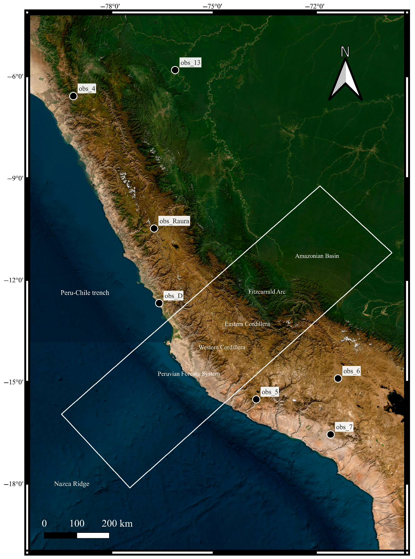
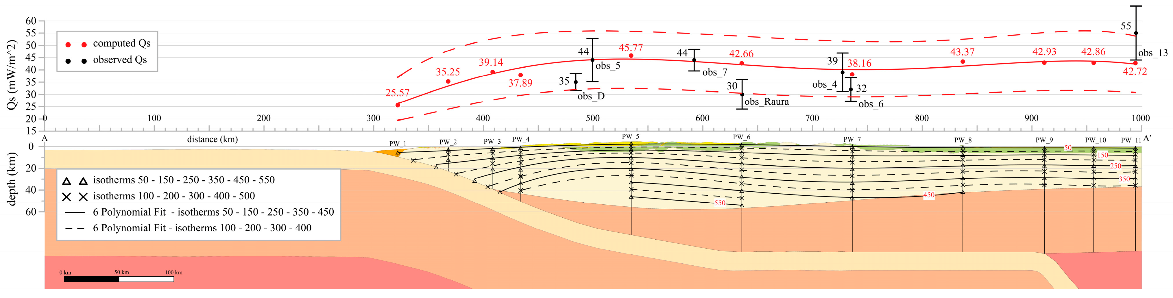
Figure 1. Localization of the study area (white box). The map shows the surface heat flow measurement sites described in Table 1.
Energies 16 07697 g001
Figure 2. Geological map of the study area based on 100 k geological maps sourced from the INGEMMET (Instituto Geológico, Minero y Metalúrgico) database.
Energies 16 07697 g002
Figure 3. Mw ≥ 6 earthquakes and their relative focal mechanism considered in the study. From the USGS [33] and Global CMT catalogues [37].
Energies 16 07697 g003
Figure 4. Lithospheric model across the study area with the location of the 11 pseudo-wells. Moho and slab geometry are based on available geophysical information [3,8,27,28,29,30,31,32]. Focal mechanisms are referred to the earthquakes shown in Figure 3 projected in the cross section.
Energies 16 07697 g004
Figure 5. Sketch of the layers used in the analytical procedure (the parameters are listed in Table 2).
Energies 16 07697 g005
Figure 6. Computed geotherms related to the 11 pseudo-wells shown in Figure 4.
Energies 16 07697 g006
Figure 7. The heat flow Qs values (red dots) are interpolated by a 6-degree polynomial (solid red line) to identify the trend along the cross-section. A graphic comparison with the observed data (black dots), and their relative errors (black bars), is realized by considering the maximum and minimum variation values of some parameters (radiogenic heat production, heat flow, and the slab dip) in the computation of the heat flow (dashed red lines). The isotherms are represented in the section with a step of 50 °C (dashed and solid black lines).
Energies 16 07697 g007
Table 1. Surface Heat Flow Sites in Peru from Uyeda et al. [16] and Henry and Pollack [17].
AcronymSite NameS LatW LongObserved Qs (mW/m2)
obs_RauraRaura10°29′76°45′30 ± 6.0[16]
obs_DCondestable12°41′76°36′35 ± 3.5[17]
obs_4La Granja6°35′79°07′39 ± 7.8[17]
obs_5Marcahui15°31′73°45′44 ± 8.8[17]
obs_6Tintaya14°54′71°21′32 ± 4.8[17]
obs_7Cerro Verde16°33′71°34′44 ± 4.4[17]
obs_13Yurimaguas5°49′76°08′55 ±11.0[17]
Disclaimer/Publisher’s Note: The statements, opinions and data contained in all publications are solely those of the individual author(s) and contributor(s) and not of MDPI and/or the editor(s). MDPI and/or the editor(s) disclaim responsibility for any injury to people or property resulting from any ideas, methods, instructions or products referred to in the content.

