Prediction of CO₂ in Public Buildings

Abstract

Heritage from the COVID-19 period (in terms of massive utilization of mechanical ventilation systems), global warming, and increasing electricity prices are new challenging factors in building energy management, and are hindering the desired path towards improved energy efficiency and reduced building consumption. The solution to improve the smartness of today’s building and automation control systems is to equip them with increased intelligence to take prompt and appropriate actions to avoid unnecessary energy consumption, while maintaining a desired level of air quality. In this manuscript, we evaluate the ability of machine-learning-based algorithms to predict CO₂ levels, which are classic indicators used to evaluate air quality. We show that these algorithms provide accurate forecasts (more accurate in particular than those provided by physics-based models). These forecasts could be conveniently embedded in control systems. Our findings are validated using real data measured in university classrooms during teaching activities.

1. Introduction

1.1. Motivation

The importance of indoor air quality has seen renewed interest following the COVID-19 outbreak, as frequent air changes have been identified as one of the most effective non-medical interventions to mitigate the spread of the virus [1]. As the occupancy of public buildings (like universities, hospitals, and shopping malls) is returning to pre-pandemic levels, the effects of COVID-19 are still noticeable in the operation of heating, ventilation, and air conditioning (HVAC) systems [2]. Indeed, the set of rules and policies introduced to preserve a safe indoor environment and mitigate the probability of contamination in closed areas have remained active in many countries as general guidelines to maintain healthy indoor environments [1]. Most notably, an example of this is the continuous use of mechanical ventilation—often at full power—when a building is occupied [3]. Indeed, while mechanical ventilation was initially enforced to reduce infection risk in indoor environments, it is now recognized as playing a pivotal role in improving overall air quality in general [4,5], which is relevant for the well-being, health, and productivity of building residents.

Mechanical ventilation, however, is also very expensive compared to indoor air recirculation strategies, especially during winter/summer times, when the use of ventilation devices needs to be compensated with extra heating or air conditioning actions to maintain the desired indoor temperature. From this perspective, the recent worldwide significant rises in energy bills have only exacerbated the need to balance the increasing utilization of ventilation strategies with energy efficiency measures, and with the interest of decreasing energy consumption.

One way to easily accommodate increased expectations in air quality with the reduction in energy consumption is to utilize innovative building management systems (BMSs) [6,7,8]. Indeed, conventional control measures have been tailored to guarantee appropriate air quality in the worst-case scenario in a building—for example, during peak hours, when the number of people inside reaches the highest values. However, this approach may result in a waste of energy during most of the day if lower levels of occupancy are experienced. Conversely, new BMSs monitor relevant air quality variables in real time, and switch on HVAC actuators only when poor levels of air quality are observed. For instance, CO₂ concentration is frequently used as a proxy to estimate air quality, and mechanical ventilation systems may be switched on when CO₂ exceeds a given concentration level (e.g., 1500 ppm). Simple strategies based on observed levels of CO₂ are indeed effective at decreasing the utilization of HVAC systems while guaranteeing that air quality does not fall below a desired threshold.

Such strategies, however, suffer from two main drawbacks: (i) first, the control action is only a reaction to a measured quantity (e.g., CO₂ concentration). Conversely, it may be more convenient to predict in advance the expected dynamics of air quality and take preemptive measures to anticipate the reaching of undesired levels of CO₂ concentrations. In many buildings (e.g., universities, shopping malls), the flow of people can often be predicted as they follow regular patterns (such as weekdays vs. festive days, times of peak occupancy vs. times of low occupancy). As a result, high levels of CO₂ frequently occur around the same times of the day or week. Predictive methods that utilize historical air quality data, if available, would enable BMSs to take more effective measures than reactive methods based solely on monitored data. Predictive methods also have two key advantages: firstly, they can anticipate high levels of CO₂, and secondly, they can help in deciding the most effective control action when high levels are observed (e.g., whether to open windows for natural air exchange or to activate mechanical ventilation systems). While natural ventilation is generally the cheapest solution, it may not always be sufficient to restore desired levels of CO₂, or it may actually become more expensive if the outdoor air is at a significantly different temperature than the indoor air, and heating/cooling systems would have to be activated to maintain the desired indoor temperature.

Accordingly, in this manuscript, we investigate, develop, and compare different algorithms to predict CO₂ levels in indoor environments, with the ultimate goal of embedding such predictions in control systems, making them more effective than simpler systems that rely solely on measured data; we aim to use these predictions to evaluate two possible alternative control actions (using natural or mechanical ventilation systems) in order to select the most convenient one. In particular, we compare a classic model developed on the physics of the system and more recent machine learning algorithms to establish their ability in the prediction task. The prediction capabilities are then evaluated on data measured in a university classroom.

1.2. State of the Art

As we have already mentioned, COVID-19 has exacerbated the issue of energy efficiency in buildings [1] and has contributed to renewing the interest of the energy community in developing prediction algorithms for CO₂ levels and air quality [9]. In general, due to the complexity of air quality evolution and the large number of influencing factors, machine learning algorithms (also known as black-box models) are increasingly becoming the most popular tool for predicting air quality parameters in various fields [10,11,12,13]. A comparison of various machine learning techniques in predicting CO₂ levels in a room was performed in [10]. The authors in [11] also tested different machine learning methods based on historical data on temperature, humidity, and room activity to assess the effect of different forecasting and history window time frames, as well as the impact of multiple sensor modalities. A deep reinforcement learning-based control to maintain acceptable air quality levels with the least energy consumption was proposed in [14]. The algorithm considered the best prediction among machine learning methods to estimate the CO₂ level and adjust the ventilation system accordingly. In [12], the authors predicted the comfort level in university premises based on CO₂ concentration, indoor temperature, and relative humidity using a Markov model, and also performed hourly CO₂ predictions based on historical CO₂ data using an LSTM network. Different variations of the LSTM method, including single-cell, stacked, and bidirectional LSTM algorithms, were used [15] to predict the CO₂ level in a bedroom of a residential building, based on occupancy and ventilation rate. In [16], the authors proposed a novel method, which integrated Bayesian optimization and empirical mode decomposition with the LSTM algorithm to improve the accuracy of CO₂ level predictions. Optimization of thermal comfort and indoor air quality in multi-zone, open spaces using extreme gradient boosting and the genetic algorithm was performed [17]. In [18] it was shown that prediction accuracy can be improved by using multiple sensor nodes for prediction. This study utilized data from spatially correlated neighboring sensors in a gated recurrent unit algorithm to predict air quality in a research laboratory. CO₂ levels were predicted using a multilayer perceptron neural network with temperature and relative humidity as inputs in reference [19]. The authors tested models with complete, partial, and zero real CO₂ concentrations available during the learning process and concluded that it is not feasible to completely omit CO₂ data from sensors and rely solely on closed-loop network predictions.

1.3. Paper Contributions

Differently from the aforementioned papers, in this paper, we provide the following contributions:

• It is widely accepted that white-box or physical models lack precision for short-time prediction; however, the benefits that data-based models may provide in comparison are not well studied. In this work, we compare machine learning algorithms with a physics-based model to appreciate the actual advantage of the first class of methodologies;
• In addition, we compare a range of data-based algorithms, starting from a simple regression algorithm, continuing with a more advanced KNN method, and finally with a sophisticated LSTM neural network, to evaluate the needs and advantages of more complex machine learning approaches;
• Finally, our case study is different from the others, as our CO₂ predictions are performed by exploiting both available historical data, as most of the other references do, but also other measured variables, such as the opening and closure of doors/windows and the full, partial, or non-utilization of mechanical ventilation devices.

2. Methodology

CO₂ levels have traditionally been used as one of many indicators to evaluate indoor air quality (IAQ). By monitoring CO₂ levels, one can assess air quality, identify poorly ventilated areas, evaluate the effectiveness of natural/artificial air-changing mechanisms, and even indirectly estimate the number of occupants in a room. Physical models were first deployed to estimate and predict the evolution of CO₂ levels in indoor environments. More recently, machine learning algorithms have been proven to be more accurate. In this section, we briefly present a physical model and some machine learning models (i.e., a regression algorithm, KNN, and LSTM), and explain how they can be tailored to the specific application of our interest. The accuracy of these models in predicting the evolution of CO₂ levels will then be evaluated in the next section, based on measured data from university buildings.

2.1. Physical Model

Physical models are usually derived by the mass balance equation of CO₂ in the indoor environment, under the assumptions of a well-mixed model with a uniform and constant concentration of CO₂ in the room, and a well-defined value of the CO₂ generation rate of the occupants of the room.

Under the previous hypotheses, in a closed volume, the increase (or decrease) of CO₂ concentration $C_{C{O}_2}$ depends directly on the number of occupants, their activity, and air change. In particular, by using an estimate of the $\dot{r}$ of CO₂ expressed in m${}^3$/s (e.g., refer to

Table 1. Typical value of CO₂ production rates as a function of the activities of individuals [20].

Type of Indoor Activity	CO2 Production Rate per Person ($\dot{\mathbf{r}}$ in m${}^{\mathbf{3}}$/s/person)
Adult people reading, seated	0.0044 $· {10}^{-3}$
Adult people seated	0.0052 $· {10}^{-3}$
or involved in light-intensity activities
Adult people standing	0.0063 $· {10}^{-3}$
or operating at medium physical activity
High-intensity physical activity	0.0174 $· {10}^{-3}$

from [20] for some values of $\dot{r}$ as a function of possible occupant activities), and knowing the volume (V) of the room, the number of occupants, $n_{occ}$, and the increase of CO₂ concentrations are related as follows:

$$V\frac{\partial C_{C{O}_2}\left(t\right)}{\partial t}=\dot{r}·n_{occ}.$$

(1)

Equation (1) may also be reformulated in terms of the volume available for each person, which can be considered an accurate variable as long as the height of the room does not exceed the other two dimensions

$$\frac{V}{n_{occ}}=\dot{r}·\frac{1}{\frac{\partial C_{C{O}_2}\left(t\right)}{\partial t}}.$$

(2)

From Equation (2), it is straightforward to observe how the variation of CO₂ concentration can be related to the number of occupants, provided that the rate of generation—which is strongly correlated with the age, activity, and behavior of the occupants—is known and constant.

If air ventilation is also considered, then the air ventilation, Q, can either be enforced with a mechanical device or may correspond to the one available under natural conditions (for instance, if windows (or doors) are open). The mass balance equation can, thus, be generalized as follows:

$$V\frac{\partial C_{C{O}_2}\left(t\right)}{\partial t}=\dot{r}·n_{occ}-Q(C_{C{O}_2}\left(t\right)-C_{ext}),$$

(3)

where Q is the air flow rate due to ventilation (either mechanic or natural) in m${}^3$/s, and $C_{ext}$ is the outdoor concentration of CO₂, which may be considered as constant. Equation (3) may be rewritten in order to explicitly estimate the indoor levels of CO₂ at time t, as follows:

$$C_{C{O}_2}\left(t\right)=C_{C{O}_2}\left(t_0\right)·e^{-\frac{Q}{V}t}+(C_{ext}+\frac{\dot{r}·n_{occ}}{Q})·(1-e^{-\frac{Q}{V}t}),$$

(4)

where $C_{C{O}_2}\left(t_0\right)$ is the level of CO₂ at some initial time $t_0$.

Finally, note that when a room is empty, the concentration decreases according to:

$$C_{C{O}_2}\left(t\right)=C_{ext}+(C_{C{O}_2}\left(t_0\right)-C_{ext})·e^{-\frac{Q}{V}t}.$$

(5)

2.2. Data-Based Models

As an alternative to the theoretical physical model introduced in Section 2.1, we now see some data-based models that are based on historical data collected during measurement campaigns, while little attention is devoted to the physics of the system. Usually, data-based models are valid alternatives when large enough observations are available, and little deviations from nominal behaviors occur, as they do not require the simplifying assumptions usually considered by physical models (e.g., the uniform and constant concentration of CO₂ or the exact knowledge of the actual production rates of the CO₂ of occupants).

2.2.1. A Simple Regression Algorithm

As a first example of a data-based model, we now consider a basic regression algorithm, where the prediction of the evolution of CO₂ is performed by simply averaging the measurements of CO₂ levels from the previous days. This is a very simple and basic estimate, and is only considered to appreciate the actual improvements that would be obtained by adopting more sophisticated prediction algorithms.

2.2.2. k-Nearest Neighbor

As a slightly more sophisticated algorithm than a basic regression algorithm, we now consider the popular k-nearest neighbor (KNN) method. KNN is a supervised machine learning algorithm that exploits the similarity between new data (in terms of explanatory variables) and already available data (historical data, which are part of the training set), to estimate the target value by averaging the available measurements. Roughly speaking, the prediction of CO₂ levels is performed by smartly averaging the historical values of CO₂ levels registered in similar conditions (i.e., the neighbors) of weather, occupancy, and HVAC utilization.

The KNN algorithm is relatively simple and easy to implement, as there is no need to build a model or make additional assumptions, and it can be applied to both classification and regression problems. The weakness of this algorithm is that it usually requires a rich historical dataset to provide accurate predictions, and the computational burden increases with the size of the dataset.

The algorithm consists of the following steps:

• Choose a number of neighbors, k, which will participate in forming the new prediction. The choice of k is not trivial, and it significantly influences the performance of the algorithm [21].
• Calculate the distance between the explanatory variables in the target case and other values in the training dataset. The classic choice as a distance measure for continuous variables is the Euclidean distance, which, for vectors $\mathbf{p}$ and $\mathbf{q}$, of length n, may be computed in terms of their components, $p_i$ and $q_i$, as follows:

  $$D(\mathbf{p},\mathbf{q})=\sqrt{{(p_1-q_1)}^2+{(p_2-q_2)}^2+...+{(p_n-q_n)}^2}.$$

  (6)
  In our application, the explanatory variables are the number of occupants in a room, whether doors/windows are open, and whether the mechanical ventilation is switched on or off (or in partial operation).
• Choose the k closest neighbors, according to the list of distances calculated in step (2), and assign weights.
• Form the prediction, by taking the average of the CO₂ measured values in the selected k historical instances. The average has to be taken in a weighted fashion, using the weights (and the neighbors) computed in step (3).

2.2.3. LSTM

As a final comparison, we consider long short-term memory (LSTM) neural networks. LSTM networks are variations of recurrent neural networks, which are particularly well-suited for handling time series data (such as CO₂ time series), as they process not only single data points but also entire sequences of data [22]. Many researchers have recently leveraged the properties of LSTM networks and have used them in applications involving time series data, such as voice recognition [23], translation [24], or weather forecasting [25]. The LSTM algorithm was initially proposed in [26] to accommodate long-term dependencies in the data. Although several variations of the LSTM method have been recently proposed [22], they usually rely on the same basic architecture, which is depicted in Figure 1 for the case with only input and output gates.

As in Figure 1, the state of the cell at time t ($c_t$) is updated in two steps: first, the input gate creates a candidate update $\widetilde{c_t}$. Then, the cell state at the next time step is obtained by appropriately combining the state at the previous time step with the update. More specifically, the basic algorithm can be outlined in the following way:

$$\begin{array}{c}{i}_t=\sigma (W_{ih}{h}_{t-1}+W_{ix}{x}_t+b_i),\end{array}$$

(7)

$$\begin{array}{c}\widetilde{c_t}=tanh(W_{\tilde{c}h}{h}_{t-1}+W_{\tilde{c}x}{x}_t+b_{\tilde{c}}),\end{array}$$

(8)

$$\begin{array}{c}{c}_t=c_{t-1}+i_t\odot \widetilde{c_t},\end{array}$$

(9)

$$\begin{array}{c}{o}_t=\sigma (W_{oh}{h}_{t-1}+W_{ox}{x}_t+b_o),\end{array}$$

(10)

$$\begin{array}{c}{h}_t=o_t\odot tanh{c}_t.\end{array}$$

(11)

where $c_t$ is the cell state, $x_t$ is the input, $h_t$ is the output, and $W_i,W_{\tilde{c}},W_o$ and $b_i,b_{\tilde{c}},b_o$ represent classic weights and bias values.

Equations (7) and (8) are responsible for computing the update vector ($\widetilde{c_t}$). Next, the previous cell state $c_{t-1}$ is updated by combining the new candidate vector ($\widetilde{c_t}$), multiplied element-wise by vector $i_t$ (Equation (9)). Here, we use the ‘⊙’ symbol to denote the element-wise product of vectors.

Finally, Equations (10) and (11) refer to the output gate, where first a sigmoid layer selects the output of the cell state, and then tanh converts the values into the range between $-1$ and 1, and multiplies them by the output of the sigmoid gate.

3. Case Study

Our case study involves a lecture hall at the University of Pisa, as shown in Figure 2, during morning classes. The lecture hall is located on the ground floor, its maximum allowed occupancy is 140 people, and the volume of the room is 438 m${}^3$. There are two windows and four doors—two internal ones (both leading to the corridor of the building) and two emergency doors (leading to an external courtyard), which are closed during the normal utilization of the room.

We formed our dataset by collecting measurements over 10 different days, during the lectures of the same professors from 8:30 to 12:30. The time step of the measurements was 10 min, resulting in a total of 40 h of records, and about 240 samples overall. The data were collected during classes of the same professors, with the objective of maintaining similar conditions (e.g., in terms of the number of students in the room, and their activity during the classes). The measurements were recorded using a system of sensors operating on Z-wave technology (the sensors are shown in Figure 3), which is a radio frequency protocol primarily used in residential buildings [27]. Devices working on Z-wave create a mesh network to communicate with each other, enabling wireless control of smart home devices via smartphone or computer. For the current study, the measurements were conducted using sensors from [28]:

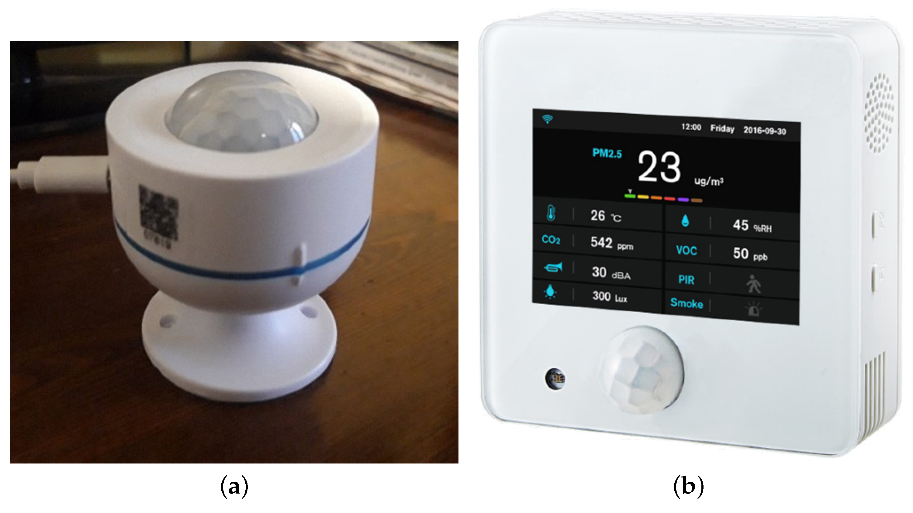
• Multisensor 9 in 1 SmartDHOME: It measures temperature (°C), brightness (lx), CO₂ (ppm), humidity (%), particulate matter ($\mathsf{\mu }$g/m${}^3$), volatile organic compounds (ppb), noise pollution (dB), movements, and the presence of smoke.
• Multisensor 4 in 1 SmartDHOME: It measures temperature (°C), luminosity (lx), humidity (%), and movements.

The monitored data from both sensors were available via the MyVirtuoso Home application. Two sensors placed in two different positions in the room were deployed to read the values of CO₂, but no significant differences were noticed. For this reason, we shall report the sequence of CO₂ values from a single sensor.

In addition, the number of people inside the room and their activity, according to Table 1, the state of the windows and doors (open, closed, half-open), and mechanical ventilation (switched on, switched off, switched on at half power) were also monitored. All recorded profiles of CO₂ levels are summarized in Figure 4, where two different background colors indicate the two different classes (with a different number of students) and the white background corresponds to breaks. From Figure 4, it is possible to appreciate that, as one may easily expect, all CO₂ time series exhibit the same behavior: the level of CO₂ increases gradually until there is a 10-minute break in the lesson, when the doors are open and students leave the room for a short walk or coffee. Accordingly, the 4 h of lessons have four peaks, followed by steep decreases corresponding to breaks or the end of classes. Also, it is possible to see from Figure 5 that fewer students attend the second two hours of classes (i.e., from 10:30 to 12:30) compared to the first two hours (i.e., from 8:30 to 10:30). In fact, the peaks of CO₂ during the second part of the morning reach lower values. On the other hand, all curves are slightly different due to the fact that, on some days, mechanical ventilation was switched on, off, or was partially working (different colors refer to different mechanical ventilation operations). In addition, in some cases, doors or windows were also open, the number of students was not constant, lesson breaks occurred at slightly different times, and class activities were different. For example, Figure 6 illustrates the effect of open windows on CO₂ concentrations on days 8 and 10. Even if—on both days—the ventilation system was not operating, and the number of students in the first lectures was approximately the same (see Figure 5), the opening of windows on day 10 (starting from 9:20) significantly flattened the CO₂ levels around the second morning peak. Conversely, day 8 experienced a significantly higher second peak of CO₂ due to the windows being closed, indicating a lack of natural ventilation. Finally, indoor and outdoor temperature and humidity also varied on different days. All the aforementioned factors make the prediction tasks quite challenging.

3.1. Algorithm Setup and Model Training

We will now briefly describe how the algorithms described in Section 2 have been tailored for the specific application of our interest. In particular, in all cases, we predicted the level of CO₂ for each day in the dataset, using the other 9 days as the training set. Specifically, the training set was utilized to fit/train the algorithms.

Remark 1.

Our choice of the training/test set was made to exploit the scarce data at our disposal as much as possible. In this way, we sometimes predicted the CO₂ levels of one day by using a historical dataset based on data that were actually recorded in future days. While we are aware that this strategy is not recommended or correct in some cases, in our case, it was possible to do so since the ten time series of the ten days did not exhibit temporal trends.

KNN and LSTM require more inputs than the regression algorithm. In particular, they provide an estimate of the CO₂ levels for the entire morning based on the following data:

• The initial concentration of CO₂ at the beginning of the day;
• The time series of the state of the doors during the morning. This information is coded as a real number equal to ‘0’ if all doors are closed, as ‘1’ if they are open, and as ‘0.5’ if only one door is open;
• The time series of the state of the windows during the whole number. Similar to the doors, it is coded with a real number, ranging from 0 to 1;
• The time series of the number of people in the room during the whole morning;
• The sequence of the state of the ventilation system, which again is coded with a real number ranging from 0 to 1, depending on the rate of the ventilation system’s operation power. Here, ‘0’ corresponds to the mechanical ventilation switched off.

The same information was also used by the physical model, where, with reference to Table 1, we further assumed that the physical activity of students was “reading seated”, while the professor was involved in “light intensity activity”. The input layer of the LSTM network includes four features—occupancy, states of doors, windows, and ventilation. It is followed by two LSTM layers, with a number of hidden neurons equal to 64, and the final output layer (with a linear activation function) has one neuron. The number of epochs was fixed at 200. The LSTM network was implemented by using the Keras deep learning package [29].

The KNN algorithm was implemented by assessing the similarity of CO₂ in the previous 30 min (or less for the first minutes of prediction) and the same four features (occupancy, states of doors, windows, and ventilation) were used to make a one-step CO₂ prediction. The number of neighbors (k) was chosen based on the best MAPE of prediction for the number of neighbors, ranging from 1 to 20 (see Figure 7), and set equal to 10.

In all cases, we first normalized the training dataset to obtain a set with zero mean ($\mu$) and unitary standard deviation ($std$):

$$x_{norm}=\frac{x-\mu }{std}.$$

(12)

The control devices (doors, windows, and mechanical ventilation) were not controlled, but only observed. This is due to the fact that an external company is currently responsible for operating the HVAC devices, but in the near future, we plan to consider them as controllable variables. For this reason, it is important to predict how CO₂ levels vary under each condition, so that the most convenient control action can be automatically taken based on the different predictions of future CO₂ levels. For instance, the energy manager of the building may decide whether to open the windows, switch on mechanical ventilation, or keep all windows closed and the mechanical ventilation switched off, based on the prediction of how CO₂ would evolve in each case and whether it would exceed a prescribed threshold value.

3.2. Evaluation Metrics

The performance of the algorithms is assessed using the following indicators:

• Root mean square error (RMSE):

  $$RMSE=\sqrt{\frac{1}{n}\sum _{i=1}^n{(y_i-\widehat{y_i})}^2}$$
• Mean absolute percentage error (MAPE):

  $$MAPE=\frac{1}{n}\sum _{i=1}^n|\frac{y_i-\widehat{y_i}}{y_i}|\ast 100,$$
• Coefficient of determination (R²):

  $$R^2=1-\frac{{\sum }_{i=1}^n{(y_i-\widehat{y_i})}^2}{{\sum }_{i=1}^n{(y_i-\overline{y})}^2},$$

where $y_i$ and $\widehat{y_i}$ correspond to the measured and predicted values at each sample instant i (i.e., every 10 min), respectively, and $\overline{y}$ is the average value of the $y_i$ values. As usual, lower values of RMSE and MAPE refer to a better prediction accuracy, while R² lies between 0 and 1, and a higher value corresponds to a better prediction.

4. Results and Discussion

In this section, we summarize the outcome of the comparison between the different prediction strategies.

4.1. Machine Learning Algorithms Outperform the Physical Model

We first observe that all machine learning algorithms, including the simple regression algorithm, outperform the physical model. As a significant example, we show the comparison between the physical model, LSTM, KNN, and regression algorithms in Figure 8. During this day, the ventilation system was operating at full power, and the number of students attending the lectures ranged between 77 and 106. For the presented case, the MAPEs for the LSTM, KNN, and regression algorithms are 13%, 16%, and 24%, respectively, while the error of the physical model is 38%. The CO₂ concentration trend modeled by the physical method is similar to the measured one. There are four peaks during the lecture period, followed by drops during the breaks, and the concentration of CO₂ increase is reflected correctly. However, there is a clear delay in the peaks (and drops) predicted by the physical model that can be motivated by the difficulty in accurately modeling the quick changes in CO₂, most likely due to the simplifying air lumping assumption underlying the physical model (and also, the difficulty in correctly modeling rates of air exchanges with the external environment). Such delayed prediction of CO₂ changes may in turn lead to delayed and, thus, less efficient, control actions. Moreover, at 9:40, the physical model overestimates the level of CO₂ by 132%, while the LSTM and KNN algorithms overestimate it only by 17% and 32%, respectively. Such an overestimation by the physical model could trigger increased utilization of mechanical ventilation or the opening of windows, while in reality, the CO₂ level would not exceed 1300 ppm. This pattern is also observed on other days in the dataset. In Figure 8, it is also possible to note that the regression algorithm overestimates the first peak, since it does not use the information that the mechanical ventilation is in operation (while all other methods do use this information).

4.2. Comparison between LSTM, KNN, and Regression

The 10-day averages of prediction errors for LSTM, KNN, and Regression are presented in

Table 2. Average prediction accuracy for 10-days.

	MAPE, %	RMSE, ppm	R2
Regression	24	347	0.69
LSTM	18	253	0.79
KNN	22	290	0.71

. The best performance was achieved by the LSTM algorithm with a MAPE of 18%, RMSE of 253 ppm, and R² of 0.79. KNN showed slightly worse results with MAPE equal to 22%, RMSE equal to 290 ppm, and R² equal to 0.71. Finally, the MAPE/RMSE/R² of regression is 24%/247 ppm/ 0.69. Day-by-day errors are shown in Figure 9. The MAPE of LSTM predictions varies between 13% and 25%, for KNN it ranges from 14% to 29%, and for the regression algorithm, it ranges from 14% to 35%.

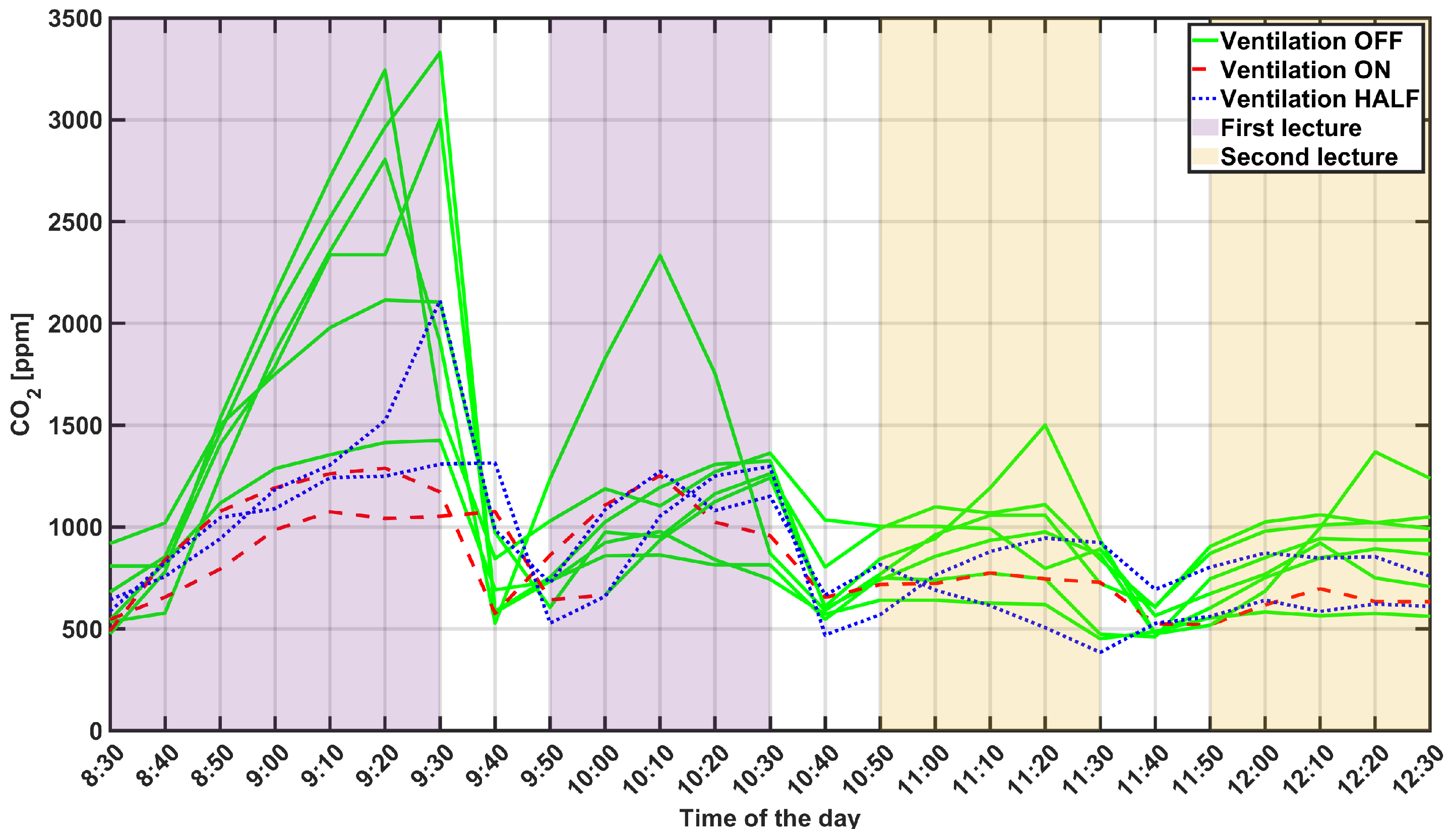
4.3. A Comparison of Different Environmental Conditions

We now compare the different algorithms in different settings: a new time series was recorded for the same classroom during an exam, with a significantly smaller number of students (only 60). The exam lasted approximately 1 h and 20 min, and during that time, students were not allowed to stand up or leave the room. The ventilation system was operating at full load throughout the whole time period. This case study presents a situation that was not present in the historical dataset and, thus, may be used to evaluate the ability of the different algorithms to generalize their predictions, or in other words, to work in different conditions than those where they have been trained. The predictions of LSTM and KNN for this dataset are presented in Figure 10. As one can easily expect, the regression algorithm makes significant prediction errors, as its prediction is based on the (different) historical dataset, and it does not exploit the information of the different environmental conditions (MAPE of 105%). LSTM and KNN provide significantly improved accuracies, and again, LSTM (MAPE of 14%) exhibits a better generalization ability to work in different environmental conditions than KNN (MAPE of 24%).

4.4. Final Discussion

A generalization of the methodology and the obtained results is obviously an important concern. In fact, one would want the procedure to be reproducible in any other classroom, and possibly in other non-scholastic public buildings.

In this case, the main limitation of the physical model is that it requires very accurate details about the room (such as volume and shape, the power of the ventilation system, and sizes of windows/doors to estimate volumes of air exchanges) and about the occupants (number and physical activity). Sometimes, such a piece of information is not available, but even when it is available, as in our case study, we show in Section 4.1 that only approximate predictions may be obtained anyway (i.e., due to the simplifying lumping assumption of the air mass).

Conversely, the machine learning approaches we tested provide more accurate predictions in a more flexible way. Moreover, the price to pay is that an adequate historical dataset needs to be available. However, as we have shown, it is very simple to equip rooms with the required sensors—which may be wireless, as in our case study—and only 7–10 days of data may be enough to provide accurate predictions. Also, the time series of one classroom may be used to make predictions for the same classroom in a different scenario (e.g., with a greatly reduced number of students). For example, Section 4.3 investigates this situation and shows that ML algorithms exhibit nice generalizability properties.

5. Conclusions

Heritage from the COVID-19 period, marked by the extended utilization of mechanical ventilation systems, along with global warming and increasing prices, are factors that hinder the path towards improved energy efficiency and reduced building consumption. The solution is to minimize energy consumption and use it only when strictly necessary, by equipping buildings with sensors and advanced control systems (e.g., BACS). However, such strategies are reactive in nature and do not exploit possibly available past measurements (e.g., to select the most appropriate control strategy).

In this manuscript, we explore the ability of machine learning algorithms to predict CO₂ levels and, thus, provide an accurate proxy of air quality. Such algorithms could be conveniently embedded within BACS, in order to enhance their capability to actively choose the best control action (e.g., whether to use mechanical or natural ventilation systems).

In particular, in this manuscript, we show that machine learning algorithms are more accurate than the models based on the physics of the system, as the latter are good at predicting average air quality behavior in the long term, but provide wrong predictions in the short term (which are the kinds of predictions that are required by real-time BACS). Conversely, LSTM and KNN algorithms have been shown to provide good predictions even with a limited historical dataset and under environmental conditions significantly different from those in the historical data. In particular, LSTM algorithms are more sophisticated and require some time for training, but they outperform KNN solutions. All our results have been tested on real data measured in university classrooms.

The next step of our work is to embed these machine learning algorithms directly within the control system, to evaluate the actual benefits in terms of decreased energy consumption, with respect to classic hysteresis-based CO₂ control systems in BACS.

References

1. Moghadam, T.T.; Ochoa Morales, C.E.; Lopez Zambrano, M.J.; Bruton, K.; O’Sullivan, D.T.J. Energy efficient ventilation and indoor air quality in the context of COVID-19—A systematic review. Renew. Sustain. Energy Rev. 2023, 182, 113356. [Google Scholar] [CrossRef] [PubMed]
2. Franco, A.; Crisostomi, E. HVAC Systems Operation Control Based on Indirect Occupant-Centric Method for Ensuring Safety Conditions and Reducing Energy Use in Public Buildings after COVID-19. Available online: https://ssrn.com/abstract=4440539 (accessed on 2 July 2023). [CrossRef]
3. Ventilation in Buildings. Available online: https://www.cdc.gov/coronavirus/2019-ncov/community/ventilation.html (accessed on 1 August 2023).
4. Lim, A.Y.; Yoon, M.; Kim, E.H.; Kim, H.A.; Lee, M.J.; Cheong, H.K. Effects of mechanical ventilation on indoor air quality and occupant health status in energy-efficient homes: A longitudinal field study. Sci. Total. Environ. 2021, 785, 147324. [Google Scholar] [CrossRef]
5. Franco, A.; Schito, E. Definition of optimal ventilation rates for balancing comfort and energy use in indoor spaces using CO2 concentration data. Buildings 2020, 10, 135. [Google Scholar] [CrossRef]
6. Taheri, S.; Razban, A. Learning-based CO2 concentration prediction: Application to indoor air quality control using demand-controlled ventilation. Build. Environ. 2021, 205, 108164. [Google Scholar] [CrossRef]
7. Li, C.; Cui, C.; Li, M. A proactive 2-stage indoor CO2-based demand-controlled ventilation method considering control performance and energy efficiency. Appl. Energy 2023, 329, 120288. [Google Scholar] [CrossRef]
8. Franco, A.; Crisostomi, E.; Hammoud, M. Advanced Monitoring Techniques for Optimal Control of Building Management Systems for Reducing Energy Use in Public Buildings. Int. J. Sustain. Dev. Plan. 2023, 18, 2025–2035. [Google Scholar] [CrossRef]
9. Lu, X.; Pang, Z.; Fu, Y.; O’Neill, Z. The nexus of the indoor CO2 concentration and ventilation demands underlying CO2-based demand-controlled ventilation in commercial buildings: A critical review. Build. Environ. 2022, 218, 109116. [Google Scholar] [CrossRef]
10. Kapoor, N.R.; Kumar, A.; Kumar, A.; Kumar, A.; Mohammed, M.A.; Kumar, K.; Kadry, S.; Lim, S. Machine Learning-Based CO2 Prediction for Office Room: A Pilot Study. Wirel. Commun. Mob. Comput. 2022, 2022, 9404807. [Google Scholar] [CrossRef]
11. Kallio, J.; Tervonen, J.; Räsänen, P.; Mäkynen, R.; Koivusaari, J.; Peltola, J. Forecasting office indoor CO2 concentration using machine learning with a one-year dataset. Build. Environ. 2021, 187, 107409. [Google Scholar] [CrossRef]
12. Tagliabue, L.C.; Re Cecconi, F.; Rinaldi, S.; Ciribini, A.L.C. Data driven indoor air quality prediction in educational facilities based on IoT network. Energy Build. 2021, 236, 110782. [Google Scholar] [CrossRef]
13. Dai, H.; Huang, G.; Wang, J.; Zeng, H. VAR-tree model based spatio-temporal characterization and prediction of O3 concentration in China. Ecotoxicol. Environ. Saf. 2023, 257, 114960. [Google Scholar] [CrossRef] [PubMed]
14. Duhirwe, P.N.; Ngarambe, J.; Yun, G.Y. Energy-efficient virtual sensor-based deep reinforcement learning control of indoor CO2 in a kindergarten. Front. Archit. Res. 2023, 12, 394–409. [Google Scholar] [CrossRef]
15. Zhu, Y.; Al-Ahmed, S.A.; Shakir, M.Z.; Olszewska, J.I. LSTM-Based IoT-Enabled CO2 Steady-State Forecasting for Indoor Air Quality Monitoring. Electronics 2023, 12, 107. [Google Scholar] [CrossRef]
16. Yang, G.; Yuan, E.; Wu, W. Predicting the long-term CO2 concentration in classrooms based on the BO–EMD–LSTM model. Build. Environ. 2022, 224, 109568. [Google Scholar] [CrossRef]
17. Martínez-Comesaña, M.; Eguia-Oller, P.; Martinez-Torres, J.; Febrero-Garrido, L.; Granada-Álvarez, E. Optimisation of thermal comfort and indoor air quality estimations applied to in-use buildings combining NSGA-III and XGBoost. Sustain. Cities Soc. 2022, 80, 103723. [Google Scholar] [CrossRef]
18. Wang, X.; Yan, J.; Wang, X.; Wang, Y. Air quality forecasting using GRU model based on multiple sensors nodes. IEEE Sensors Lett. 2023, 7, 6003804. [Google Scholar] [CrossRef]
19. Khazaei, B.; Shiehbeigi, A.; Haji Molla Ali Kani, A. Modeling indoor air carbon dioxide concentration using artificial neural network. Int. J. Environ. Sci. Technol. 2019, 16, 729–736. [Google Scholar] [CrossRef]
20. Emmerich, S.J.; Persily, A.K. State-of-the-Art Review of CO2 Demand Controlled Ventilation Technology and Application. Nist Interagency/Internal Rep. (NISTIR) 2001, 12, 1–43. [Google Scholar]
21. Zhang, Z. Introduction to machine learning: k-Nearest neighbors. Ann. Transl. Med. 2016, 4, 218. [Google Scholar] [CrossRef]
22. Yu, Y.; Si, X.; Hu, C.; Zhang, J. A Review of Recurrent Neural Networks: LSTM Cells and Network Architectures. Neural Comput. 2019, 31, 1235–1270. [Google Scholar] [CrossRef]
23. Eyben, F.; Weninger, F.; Squartini, S.; Schuller, B. Real-life voice activity detection with LSTM Recurrent Neural Networks and an application to Hollywood movies. In Proceedings of the 2013 IEEE International Conference on Acoustics, Speech and Signal Processing, Vancouver, BC, Canada, 26–31 May 2013. [Google Scholar]
24. Ren, B. The use of machine translation algorithm based on residual and LSTM neural network in translation teaching. PLoS ONE 2020, 15, e0240663. [Google Scholar] [CrossRef] [PubMed]
25. Karevan, Z.; Suykens, J.A.K. Transductive LSTM for time-series prediction: An application to weather forecasting. Neural Netw. 2020, 125, 1–9. [Google Scholar] [CrossRef] [PubMed]
26. Hochreiter, S.; Schmidhuber, J. Long Short-Term Memory. Neural Comput. 1997, 9, 1735–1780. [Google Scholar] [CrossRef] [PubMed]
27. Yassein, M.B.; Mardini, W.; Khalil, A. Smart homes automation using Z-Wave protocol. In Proceedings of the 2016 International Conference on Engineering & MIS (ICEMIS), Agadir, Morocco, 22–24 September 2016. [Google Scholar]
28. SmartDHOME. Available online: https://www.smartdhome.com/ (accessed on 1 August 2023).
29. Keras: Deep Learning for Humans. Available online: https://keras.io/ (accessed on 1 April 2023).
Figure 1. Architecture of an LSTM network with only input and output gates.
Energies 16 07582 g001
Figure 2. Lecture classroom (a) and aerial image of the building (b) of the case study at the University of Pisa.
Energies 16 07582 g002
Figure 3. Multisensor 4 in 1 SmartDHOME (a) and Multisensor 9 in 1 SmartDHOME (b) used to collect data for the case study.
Energies 16 07582 g003
Figure 4. Measured CO2 profiles during the different days. Different line colors emphasize the role of the ventilation system (ON, OFF, and 50%), while the different backgrounds refer to the first class, the second class, and breaks.
Energies 16 07582 g004
Figure 5. Number of people during the first (blue) and second (orange) lectures on the different days.
Energies 16 07582 g005
Figure 6. Measured CO2 profiles for day 8 and day 10.
Energies 16 07582 g006
Figure 7. Evolution of MAPE depending on the number of neighbors, k.
Energies 16 07582 g007
Figure 8. Prediction of CO2 level for one day.
Energies 16 07582 g008
Figure 9. Prediction errors: (a) MAPE; (b) RMSE and (c) coefficient of determination R2 when a different day of the dataset is chosen as the test set.
Energies 16 07582 g009
Figure 10. Predictions for the exam day.
Energies 16 07582 g010