Numerical Simulation Method for Flash Evaporation with Circulating Water Based on a Modified Lee Model

Abstract

Flash evaporation processes are widely adopted in the desalination, food processing, waste heat recovery and other industries for heat extraction or product separation. In this paper, a pressure-driven phase transition model is developed by improving the Lee model and combined with the VOF (Volume of Fluid) method to numerically simulate the flash evaporation process. In this modified Lee phase transition model, the driving force for the rates of the local phase transition is calculated using the local temperature and static pressure magnitude. Numerical simulations are carried out in a water-circulating flash chamber and compared with the experimental results to obtain the values of the time relaxation parameters. And the non-equilibrium fraction of the outlet water can be effectively obtained under different conditions of flow rate, inlet temperature and initial liquid level height. The time relaxation factor takes values from 0.195 to 0.43 (P_out,v = 19.9 kPa) and from 0.31 to 0.92 (P_out,v = 31.2 kPa) with increasing superheat. In addition, the model can effectively represent the evolution of the unstable flow flash evaporation from the initial rapid boiling state to dynamic equilibrium.

1. Introduction

Flash evaporation is a violent boiling phenomenon in which a portion of a high-pressure liquid undergoes a phase change to produce vapor as a result of a sudden reduction in pressure. Compared to traditional evaporation methods, flash evaporation is faster and can cause the liquid to phase change without raising the temperature of the workpiece. As a result, flash evaporation plays an important role in industrial production processes, including desalination, wine processing, geothermal energy utilization and waste heat recovery [1].

Since the 1970s, scholars have carried out systematic parametric and mechanical studies to analyze the flash evaporation process of water, and the flash evaporation process with a single steam outlet (static flash evaporation) was first studied and is more fully characterized and understood [2,3,4,5]. Miyatake et al. [2] experimentally investigated the static flash evaporation of water in a closed chamber with a diameter of 8 cm, where a rapid boiling stage and a slow surface evaporation stage were presented and measured in duration (within the superheat of 0–44 °C and saturation temperature of 40–80 °C). Kim [3] experimentally investigated the static flash evaporation of water in a cylindrical chamber with a diameter of 15 cm and obtained a gradual decrease in the rate of bubble production in deep water under water pressure. This shows the important role played by water pressure in the flash evaporation process. Saury et al. [4] experimentally investigated the flash evaporation of static water in a confined chamber of 30 cm diameter. The variation in phenomena, phase transition rate and duration under different conditions was stated, and further, the important effect of the rate of pressure drop on the outlet was illustrated (within the initial liquid level of 25–250 mm, vacuum pressure of 50–150 mbar, superheat of 0–44 °C, pressure drop rate of 0–3.5 bar/s).

Compared to a static flash evaporation processes, flow flash evaporation processes accompanied by circulation of the working medium are more widely used and have better research value. This is due to the temperature of the flash chamber being maintained at a steady state, and steam can be produced continuously by hot medium replenishment at the inlet and the temperature drop due to the phase change. A series of experimental studies have been carried out by scholars to investigate the steam production characteristics of flow flash evaporation under different operating conditions [6,7,8,9]. Yan et al. [6] experimentally investigated the heat and mass transfer characteristics of two kinds of flash evaporation processes, static flash evaporation (in a space of 0.13 × 0.125 × 0.5 m) and flow flash evaporation (in a space of 0.17 × 0.5 × 0.5 m). The authors regarded the flowing flash evaporation process as a kind of continuous static flash evaporation, the sudden rise of the heat transfer coefficient at the beginning of the flow flash evaporation was illustrated and the degree of flash evaporation was measured (within the inlet superheat of 1.5~19 K and liquid film height of 0~0.3 m). Zhang et al. [7] experimentally investigated the variation of the non-equilibrium fraction defined in terms of inlet and outlet superheat (within the inlet superheat of 2~30 K, initial level height of 0.1~0.3 m, pressures of 0.0074~0.07 MPa, and water flow rate of 400–1400 L/h). El-Dessouky et al. [8] experimentally investigated the flash evaporation efficiency and heat transfer coefficients for different multi-stage flash evaporation processes with different types of inter chamber orifices, work mass superheat (0.6–12.3 K), and liquid level heights (0.1–0.95 m).

Due to the rapidity of phase transitions occurring in flash chambers and the difficulty of internal measurements, experimental studies are still not clear enough to investigate the complex heat and mass transfer processes. Many scholars have used various numerical methods to simulate the flow flash evaporation in order to obtain the more detailed heat and mass transfer mechanisms and the steam generation rate at different operating conditions or in different flash chambers, as described below. Seul and Lee [10] used the Eulerian method to simulate liquid-phase flow and the Lagrangian method to simulate bubble motion, and used the difference between the droplet temperature and the saturation temperature as the driving force for the growth of the bubble particles. The saturation temperature is determined by the distance of the particles from an assumed fixed free interface, whereas the liquid level height varies very drastically during the actual flash evaporation process. Jin and Low [11] used a single-phase model to investigate the distribution of flow fields within the flash evaporation chamber. Dietzel et al. [12] investigated three different models of phase transition in a flash evaporation process in the system based on Eulerian–Eulerian two-phase flow, with mass transfer rates being calculated by local vapor and saturation pressure differences, entropy and saturation entropy differences, and local heat transfer rates, respectively. The single bubble growth process under different models was compared in the study, but the reliability of the calculations in simulating the flash evaporation was not investigated by applying them to a pool flash evaporation. Chen and Zhang [13] simulated two-phase flow in a flash chamber using a Eulerian–Eulerian model and investigated the effects of different superheat, pressures, inlet mass flow rates and flash chamber models on the efficiency of the flash evaporation process. The rate of mass transfer is controlled in the model using the amount of heat transfer from the gas and liquid to the interface, which requires setting the convective heat transfer coefficients for the two heat transfer processes separately.

Some of the scholars’ simulation studies are based on the VOF method. Nigim and Eaton [14] used a VOF based numerical model to simulate a two-dimensional flash evaporation process with the incompressible and steady flow assumption and used the Lee model (with a coefficient of 0.1) and generalized Rayleigh–Plesset equation (with generalized bubble radius of 10⁻⁶, vaporization coefficient of 50 and nucleation volume fraction of 0.0005) to simulate the mass transfer process together. But the authors’ steady-state calculations under the stability assumption do not allow the model to predict transient changes in flash evaporation. Lv et al. [15] carried out numerical simulations based on the VOF model, and six different flash chambers with spoiler were compared at different pressures and salt contents. The mass transfer in the above article is calculated based on the initial temperature, initial total volume of the liquid and the current rate of temperature change.

At present, there are several numerical studies on transient flow flash evaporation, and the significant effect of pressure on the mass transfer rate is not considered. Therefore, in this paper, a transient, VOF-based, modified pressure-driven Lee numerical model is proposed to simulate the flow flash evaporation process. By calculating the mass transfer using local temperature and local pressure, the effect of water pressure, which increases the saturation temperature of the bottom water and inhibits local phase transition, is taken into account. The accuracy of the model is verified by several sets of numerical simulations. And the time-dependent flash evaporation process from initiation to dynamic equilibrium is analyzed.

2. Mathematical Approach

2.1. Physical Model and Boundary Conditions

The chamber with horizontal flow is studied in this paper, as shown in Figure 1. The basic horizontal flash chamber has three openings, and the walls are considered to be non-slip and adiabatic.

During the working process, the water with a temperature of T_in enters the flash chamber through inlet 1 at a mass flow rate of q_m,w. The pressure at vapor outlet 1 (P_out,v), which is lower than the saturation pressure corresponding to T_in, maintains a low pressure in the flash chamber and drives the flash evaporation process. The liquid outlet 2 is set as a pressure boundary (P_out,l) to maintain the liquid level at a certain height, whose magnitude can be calculated from the initial liquid level h and P_out,v.

The thermophysical properties of water and vapor at various temperatures are detailed in

Table 1. Thermophysical properties of saturated water and vapor at 19.9/31.2 kPa.

Materials	ρ	λ	cp	μ
Water (19.9 kPa)	983.16	0.65100	4185.1	0.00046602
Water (31.2 kPa)	977.73	0.65972	4190.2	0.00040353
Vapor (19.9 kPa)		0.02104	1964.8	0.00001085
Vapor (31.2 kPa)		0.02186	1986.2	0.00001120

, where ρ represents the density of mixture, c_p represents the specific heat, λ represents the thermal conductivity and μ represents the dynamic viscosity. The thermophysical properties of water are considered as constant values corresponding to P_out,v, while the vapor is treated as an ideal gas to calculate its density at different local temperatures and pressures.

2.2. Governing Equations

In this paper, a two-part set of governing equations were used to numerically simulate the flash evaporation process of pure water flow, as shown in Figure 2.

The two-phase distributions and flow states at each transient are obtained by the equations of transient momentum conservation, mass conservation, energy conservation and the phase fraction equation of the VOF method, which are solved sequentially as shown on the left side of the Figure 2. And the phase transition from liquid to vapor is modeled by the modified pressure-driven Lee model, in which the phase transition rate is not calculated from the difference between the local temperature and the fixed saturation temperature, but using the local pressure and temperature, and the source term updates are controlled to ensure the convergence of calculations, as shown on the right side of the Figure 2.

Equations (1)–(3) represent the conservation equations for mass, momentum and energy. The equations calculate only a single value of pressure, velocity or temperature at each position, shared by both the liquid and gas phases.

$$\frac{\partial \rho }{\partial t}+\nabla \cdot \rho \mathit{v}=0$$

(1)

$$\frac{\partial }{\partial t}(\rho \mathit{v})+\nabla \cdot (\rho \mathit{vv})=-\nabla p+\nabla ·\mu (\nabla \mathit{v})+\rho \mathit{g}+{\mathit{F}}_{\mathrm{C}S\mathrm{F}}$$

(2)

$$\frac{\partial }{\partial t}(\rho E)+\nabla \cdot [(\rho E+p)\mathit{v}]=\nabla ·(\lambda \nabla T)+{\dot{S}}_{\mathrm{lv}}$$

(3)

where t represents time, p represents pressure, v represents the velocity vector, g represents the gravitational acceleration vector, E represents the internal energy, T represents the local temperature and ${\dot{S}}_{\mathrm{lv}}$ is the source terms of energy.

The density of the vapor is calculated by the following Equation (4), which is updated before each calculation step.

$${\rho }_{\mathrm{v}}=p{\mathrm{M}}_{\mathrm{w}}/\mathrm{R}T$$

(4)

where M_w is taken as 0.018 kg/mol, representing the molar mass of water, and R is taken as 8.314 J/(mol∙K), representing the ideal gas constant.

The F_CSF is the source term in the momentum conservation equations that express the surface tension as a volumetric force, as shown in Equation (5) below. Its representation is derived from the continuum surface force model proposed by Brackbill et al. [16]. In this model, the surface tension is assumed to be constant across the surface and only the normal force is considered. The pressure drop across the surface is determined by the surface tension coefficient σ and the curvature of the interface κ. And the conversion to a volumetric force is achieved by deriving the divergence theorem.

$${\mathit{F}}_{\mathrm{CSF}}=\sigma \frac{\rho \kappa \nabla \alpha }{0.5({\rho }_{\mathrm{l}}+{\rho }_{\mathrm{v}})}$$

(5)

$$\kappa =\nabla ·\frac{\nabla \alpha }{|\nabla \alpha |}$$

(6)

Through the solution of the partial differential equation on the phase fraction, the Volume of Fluid (VOF) method can determine the proportion of each phase within each cell, thus revealing the overall gas–liquid distribution. The relative motion of the two phases is described by changes in the local phase fraction. The phase fraction equation of the VOF method is written as follows [17].

$$\frac{\partial {\alpha }_{\mathrm{l}}{\rho }_{\mathrm{l}}}{\partial t}+\nabla \cdot ({\alpha }_{\mathrm{l}}{\rho }_{\mathrm{l}}v)={-\dot{m}}_{\mathrm{lv}}$$

(7)

where, ${\alpha }_{\mathrm{l}}$ represents the volume fraction of liquid phase, and ${\dot{m}}_{\mathrm{lv}}$ represents the mass transfer rate in units of kg/(m³∙s). The phase fraction is limited to the range of 0 to 1, and the sum of the phase fractions of the two phases is 1 within a single cell.

The magnitude of the internal energy of mixture in the energy equation is determined by the following equations.

$$E=\frac{{\alpha }_{\mathrm{l}}{\rho }_{\mathrm{l}}{E}_{\mathrm{l}}+{\alpha }_{\mathrm{v}}{\rho }_{\mathrm{v}}{E}_{\mathrm{v}}}{{\alpha }_{\mathrm{l}}{\rho }_{\mathrm{l}}+{\alpha }_{\mathrm{v}}{\rho }_{\mathrm{v}}}$$

(8)

$$E_{\mathrm{i}}=c_{\mathrm{p},i}(T-273.15\mathrm{K})$$

(9)

The density ρ, thermal conductivity λ and the dynamic viscosity μ of the mixture is calculated using Equation (10), where Φ refers to μ, ρ or λ.

$$\Phi ={\Phi }_{\mathrm{l}}{\alpha }_{\mathrm{l}}+{\Phi }_{\mathrm{v}}{\alpha }_{\mathrm{v}}$$

(10)

Furthermore, the Renormalization Group k-ε model was employed to simulate the turbulent flow in the chamber. This model is considered effective in combination with the VOF method, as indicated by Banerjee’s research, when compared to the Standard k-ε and RSM models [18]. It determines the turbulent kinetic energy within the flow by solving the k and ε equations, which are presented below.

$$\frac{\partial \left(\rho k\right)}{\partial t}+\frac{\partial \left(\rho k{u}_{\mathrm{i}}\right)}{\partial x_{\mathrm{i}}}=\frac{\partial }{\partial x_{\mathrm{j}}}(1.393{\mu }_{\mathrm{eff}}\frac{\partial k}{\partial x_{\mathrm{j}}})+G_{\mathrm{k}}+\rho \epsilon$$

(11)

$$\frac{\partial \left(\rho \epsilon \right)}{\partial t}+\frac{\partial \left(\rho \epsilon u_{\mathrm{i}}\right)}{\partial x_{\mathrm{i}}}=\frac{\partial }{\partial x_{\mathrm{j}}}(1.393{\mu }_{\mathrm{eff}}\frac{\partial \epsilon }{\partial x_{\mathrm{j}}})+\frac{C_{1\epsilon }^{*}\epsilon }{k}{G}_{\mathrm{k}}-1.68\rho \frac{{\epsilon }^2}{k}$$

(12)

where k is the turbulent kinetic energy, ε is the turbulent dissipation rate, G_k donates the generation of turbulence kinetic energy resulting from the mean velocity gradients, and μ_eff is the corrected turbulence viscosity.

Based on the above model, the values of the source terms ${\dot{m}}_{\mathrm{lv}}$ and ${\dot{S}}_{\mathrm{lv}}$ are further modeled to simulate the phase change process. ${\dot{m}}_{\mathrm{lv}}$ expresses the mass transfer from the liquid phase to the gas phase during the phase change process, and its value ultimately results in an increase in ${\alpha }_{\mathrm{v}}$ and a decrease in ${\alpha }_{\mathrm{l}}$. Additionally, the reduction in sensible heat due to evaporation is regulated by ${\dot{S}}_{\mathrm{lv}}$ in the energy equation. In this paper, the source terms within the entire computational model are provided by the modified Lee model below.

$${\dot{m}}_{\mathrm{lv}}=\left\{\begin{array}{l}c\times \frac{{\alpha }_{\mathrm{l}}{\rho }_{\mathrm{l}}(T-31.35p^{0.1526}+191.1)}{31.35p^{0.1526}+191.1}\left(T_{\mathrm{l}}>31.35p^{0.1526}+191.1\right)\\ 0\left(T_{\mathrm{l}}\le 31.35p^{0.1526}+191.1\right)\end{array}\right.$$

(13)

$${\dot{S}}_{\mathrm{lv}}=-{\dot{m}}_{\mathrm{lv}}\mathrm{r}$$

(14)

where c is the time relaxation parameters, and r represents the latent heat.

As shown above, this model first assesses whether the temperature in a cell satisfies the criteria for a phase change process, and then, it calculates the mass transfer rate from the static pressure and local temperature. This approach eliminates the need to differentiate between nucleation boiling and interfacial mass transfer by using a single process to treat the phase change phenomenon occurring at both the phase boundary cell and the liquid-filled cells, which results in a simple and effective simulation of the flow flash evaporation process.

In contrast to the original Lee model [19], the main modification in the model described above is the use of local pressure and temperature as the driving force for the source term. This modification is critical because even small pressure changes at low pressure can have a significant effect on the saturation temperature, resulting in the pressure distribution in the chamber having a large effect on the rate of the phase change. In this model, the saturation temperature is calculated from the local pressure, which makes it possible to represent the inhomogeneous distribution of vapor production rates due to the stratification of water pressure under gravity.

2.3. Solution Strategy and Numerical Approach

The Pressure-Implicit with Splitting of Operators (PISO) method is used to couple the momentum and mass equations. The equations for pressure, momentum, turbulent kinetic energy, turbulent dissipation rate and energy are in first-order windward discrete format. The gradient is obtained using the least-squares approach, which computes the approximate gradient solution of the non-square matrix equation by solving the minimization problem in a least-squares sense. The time step employed in the transient calculations is 5 × 10⁻⁵ s. Under-relaxation factors were applied with the following values: 0.3 for pressure, 0.3 for momentum, 0.8 for energy and 0.5 for turbulent kinetic energy and turbulent dissipation rate.

In addition, the study by Ding et al. shows that some numerical oscillations may occur when employing the Lee model for phase change processes [20]. The flash evaporation process is a rapid change of the liquid from a superheated thermodynamic disequilibrium to an equilibrium state, and this oscillation problem does exist due to the rapid phase transitions during the calculations of flash evaporation, even leading to a divergence in some cases.

In order to make the calculation have a better stability, an assumption is made in this paper that the local pressure does not change in a certain period of time. This assumption effectively prevents the divergence in the computation and can suppress the phenomenon of numerical oscillations that arise at certain times, as shown in Figure 3, which monitors the different variations of pressure and phase change rate with time at a certain location before and after the application of the assumptions.

In this paper, an independent validation of the pressure invariant time in this assumption is further carried out in order to avoid the inaccuracy of the calculation results caused by a long period of time for the assumption. The results of this independent validation are shown in Figure 4. The time in this assumption was eventually set to 1 ms to ensure that the calculations can converge sufficiently well with as little detrimental effect on the results as possible.

2.4. Grid Independence

A grid independence study was conducted in this work (T_in = 337.65 K, q_m,w = 9.83 kg/s, P_out,v = 19,900 Pa, P_out,l = 21,443.2 Pa) using the above model.

The mass flow rate of vapor q_m,v and the average temperature of the outlet water T_out were compared for different grids. The minimum sizes of four grids are 3.0 mm, 2.5 mm, 2.0 mm and 1.5 mm, corresponding to the number of grids 154,845, 224,000, 350,000 and 62,0712, respectively. Over the calculated time (26,000 steps, corresponding to 0~1.3 s), the mass rate of vapor generation shows the same trend and eventually tends to the same stable value as reflected in Figure 5a. In addition, the results in

Table 2. Time averaged over 1.1–1.3 s for each compared value.

Number of Grids	qm,v (kg/s)	Tout (K)
154,845	0.05089	334.207
224,000	0.05707	334.3567
350,000	0.05359	334.246
620,712	0.05341	334.243

show that the computational results for the case of the mesh with 2 mm edge are already almost identical to the results of the 1.5 mm mesh (the errors of q_m,v and T_out both occur after the third decimal place). Based on these results and taking into account the computational time, the mesh with 2.0 mm edge was selected for the subsequent numerical simulations. The local structure of the mesh is shown in Figure 5b.

3. Results and Discussion

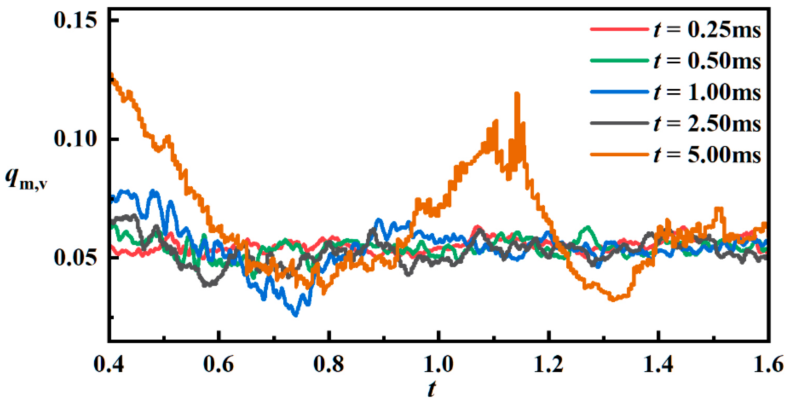
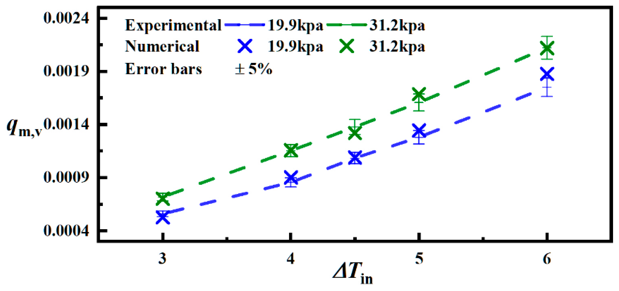
3.1. Values of Time Relaxation Parameters and Model Verification

As shown in Equation (13), the factor c plays a crucial role in the magnitude of the evaporation rate, since the magnitude of the phase transition rate is obtained by multiplying the driving force (the difference between the local and saturation temperatures) with c.

According to the differences in computational models and working conditions, different scholars have set different magnitudes for c, which can be in the order of 0.1~1000, and a frequently used selection criterion is to select c to satisfy one of the assumptions in the derivation of Lee’s model, which considers that the interfacial temperature of the bubbles is equal to the saturation temperature [21]. However, it is clear that in a flash evaporation process, the factor c cannot be determined from this criterion because the phase change process in this case is carried out in an environment surrounded by superheated water with a temperature greater than the saturation temperature. To enable the model to accurately simulate the occurrence of phase transitions during flash evaporation, the factor c in this paper was selected based on a comparison with experimental articles, and great simulation results using this model were achieved, as described below.

The width, length and height of the flash chamber in the compared experimental article are 100 mm, 100 mm and 480 [7]. The non-equilibrium fraction values obtained from inlet and outlet temperature measurements at different inlet temperatures under an initial water level height of 120 mm and flow rate of 800 L/h are given in the paper.

Ten sets of numerical simulations were conducted to fine-tune the time relaxation parameters, and the final values of c and the comparison between numerical simulation results and experimental results are shown in Figure 6 and Figure 7 below. The time relaxation factor takes values from 0.195 to 0.43 (P_out,v = 19.9 kPa, T_in = 3–6 K) and from 0.31 to 0.92 (P_out,v = 31.2 kPa, T_in = 3–6 K) as the superheat increases.

In addition, using the time relaxation parameters described above, the other eight groups of flash evaporation experiments with different superheat, initial liquid level height h or flow rate in the experiment were simulated and compared by using the model described in this paper, and the results are shown in

Table 3. Results of numerical simulation verification.

	h	qm,w	pout,v	Tin	qm,v (Numerical)	qm,v (Experimental)	Errors
Case 1	0.12	800	19.9	63.5	0.000768	0.000724	6.1%
Case 2	0.12	800	19.9	65.5	0.00158	0.00154	2.6%
Case 3	0.12	800	31.2	73.5	0.000985	0.000931	5.8%
Case 4	0.12	800	31.2	75.5	0.00189	0.00187	1.0%
Case 5	0.16	600	19.9	64.5	0.000713	0.000684	4.2%
Case 6	0.16	1000	19.9	64.0	0.00122	0.00138	11.6%
Case 7	0.16	800	19.9	64.5	0.00106	0.000989	7.1%
Case 8	0.10	800	19.9	64.5	0.00112	0.00121	7.4%

below. The errors in the table are obtained by dividing the absolute difference in q_m,v by the experimental results. It can be seen that this value-taking scheme of c has a good accuracy for the simulation of flash evaporation for different working conditions within a certain range.

3.2. Transient Flash Process

In addition, such a flash evaporation process from the initial rapid boiling state to dynamic equilibrium is simulated by the above model. For the initial conditions, a liquid level height of 0.12 m was maintained inside the flash chamber, and the water temperature was kept the same as the inlet temperature.

As the calculations begin, the low pressure of the vapor outlet starts to cause the pressure in the vapor space to decrease. The reduction of pressure around the water causes the water to reach an unbalanced state, resulting in the rapid conversion of superheated water from liquid to vapor, while part of the sensible heat contained in the water is converted to latent heat contained in the vapor, resulting in a decrease in the average temperature of the water body.

Due to the entry of hot water, the process of imbalance-to-equilibrium transition continues throughout the flash evaporation process, but as shown in Figure 8 and Figure 9a, there is a tendency for this phase change process to vary from fast to slow to dynamically stable. Specifically, in this case, the early stage of flash evaporation (t = 0~0.3 s) is the liquid level rising stage, and due to the high temperature of the water body, the large number of vapor bubbles caused by the violent phase change makes the water level rise rapidly, as shown in Figure 8a–h.

At the same time as the upper water body is being lifted up, it can be observed that the water vapor produced by the flash evaporation process cuts the upper water body in a very dispersed manner, which decreases the spatial density of the water body. This part of the uplifted broken water body at the same time has the nature of low pressure and high temperature, and the violent phase change process happens here.

Under the violent phase change process, the temperature of the water in the flash chamber is rapidly reduced, and the reduction of vapor generation makes the water body fall back. The fallback of the water column occurs in 0.3~4.0 s, accompanied by a slow decrease in the water temperature, and causes a slowdown of the flash vaporization rate and the slow movement of the liquid level downward, as shown in Figure 9b.

After t > 4.0 s, the decrease in the water temperature leads to the lowering of the driving force of the phase transition in the bottom layer, and the bubble generation phenomenon gradually changes from a uniform distribution at the beginning to a stable distribution of more steam production in the surface layer and less steam production in the bottom layer, and the steam generation rate reaches a stable value at this time.

In this state of dynamic equilibrium, there are two main areas of intense vapor production, which are located around the upper water column area due to low pressure and around the inlet area due to high temperature, as shown in Figure 10. Gravity has led to a significant gradation in the water pressure and further to a gradation in the flash evaporation rate. With the intense phase change heat absorption around the inlet and the high pressure in the bottom, there is almost no phase change occurring in the bottom water. It can be seen that the effect of pressure distribution under gravity in the flash chamber is effectively captured.

4. Conclusions

In this paper, a model combining a modified Lee model and VOF model is proposed to simulate the flash evaporation process as a result of a pressure drop. A series of transient three-dimensional flash evaporation processes accompanied by water circulation are simulated and the following conclusions were obtained.

(1)

The mass transfer process during flow flash evaporation can be effectively modeled by the modified Lee model proposed in this paper, which uses local pressure and temperature to calculate the phase transition source term.

(2)

With the time relaxation parameters ranging from 0.195 to 0.43 (P_out,v = 19.9 kPa, T_in = 3–6 K) and from 0.31 to 0.92 (P_out,v = 31.2 kPa, T_in = 3–6 K), the model can effectively simulate the equilibrium in the flow flash evaporation process under different operating conditions.

(3)

The process from the initial rapid boiling state to the dynamic equilibrium of the flow flash evaporation process can be captured by this model, and the violent phase change regions and the slow phase change regions due to water pressure can be observed, which are valuable for a better understanding of the heat and mass transfer process in a flow flash evaporation process.

References

1. Wu, H.; Liu, W.; Li, X.; Chen, F.; Yang, L. Experimental Study on Flash Evaporation under Low-pressure Conditions. J. Appl. Sci. Eng. 2019, 22, 213–220. [Google Scholar]
2. Miyatake, O.; Murakami, K.; Kawata, Y.; Fujii, T. Fundamental Experiments of Flash Evaporation. Bull. Soc. Sea Water Sci. Jpn. 1972, 26, 189–198. [Google Scholar]
3. Kim, J.-I.; Lior, N. Some critical transitions in pool flash evaporation. Int. J. Heat Mass Transf. 1997, 40, 2363–2372. [Google Scholar] [CrossRef]
4. Saury, D.; Harmand, S.; Siroux, M. Flash evaporation from a water pool: Influence of the liquid height and of the depressurization rate. Int. J. Therm. Sci. 2005, 44, 953–965. [Google Scholar] [CrossRef]
5. Gopalakrishna, S.; Purushothaman, V.; Lior, N. An experimental study of flash evaporation from liquid pools. Desalination 1987, 65, 139–151. [Google Scholar] [CrossRef]
6. Yan, J.; Zhang, D.; Chong, D.; Wang, G.; Li, L. Experimental study on static/circulatory flash evaporation. Int. J. Heat Mass Transf. 2010, 53, 5528–5535. [Google Scholar]
7. Zhang, Y.; Wang, J.; Liu, J.; Chong, D.; Zhang, W.; Yan, J. Experimental study on heat transfer characteristics of circulatory flash evaporation. Int. J. Heat Mass Transf. 2013, 67, 836–842. [Google Scholar] [CrossRef]
8. El-Dessouky, H.; Ettouney, H.; Al-Juwayhel, F.; Al-Fulaij, H. Analysis of Multistage Flash Desalination Flashing Chambers. Chem. Eng. Res. Des. 2004, 82, 967–978. [Google Scholar] [CrossRef]
9. Zhang, Y.; Wang, J.; Yan, J.; Chong, D.; Liu, J.; Zhang, W.; Wang, C. Experimental study on non-equilibrium fraction of NaCl solution circulatory flash evaporation. Desalination 2014, 335, 9–16. [Google Scholar] [CrossRef]
10. Seul, K.W.; Lee, S.Y. Numerical predictions of evaporative behaviors of horizontal stream inside a multi-stage-flash distillator. Desalination 1990, 79, 13–35. [Google Scholar] [CrossRef]
11. Jin, W.; Low, S. Investigation of single-phase flow patterns in a model flash evaporation chamber using PIV measurement and numerical simulation. Desalination 2002, 150, 51–63. [Google Scholar] [CrossRef]
12. Dietzel, D.; Hitz, T.; Munz, C.-D.; Kronenburg, A. Expansion rates of bubble clusters in superheated liquids. In Proceedings of the ILASS—Europe 2017 28th Conference on Liquid Atomization and Spray Systems, Valencia, Spain, 6–8 September 2017. [Google Scholar]
13. Chen, C.; Zhang, C. Numerical Simulation of Evaporation Characteristics of Flash Evaporation of Hot Water. Power Syst. Eng. 2020, 36, 25–28. [Google Scholar]
14. Nigim, T.; Eaton, J. CFD prediction of the flashing processes in a MSF desalination chamber. Desalination 2017, 420, 258–272. [Google Scholar] [CrossRef]
15. Lv, H.; Wang, Y.; Wu, L.; Hu, Y. Numerical simulation and optimization of the flash chamber for multi-stage flash seawater de-salination. Desalination 2019, 465, 69–78. [Google Scholar] [CrossRef]
16. Brackbill, J.; Kothe, D.; Zemach, C. A continuum method for modeling surface tension. J. Comput. Phys. 1992, 100, 335–354. [Google Scholar] [CrossRef]
17. Hirt, C.W.; Nichols, B.D. Volume of fluid (VOF) method for the dynamics of free boundaries. J. Comput. Phys. 1981, 39, 201–225. [Google Scholar] [CrossRef]
18. Banerjee, R.; Isaac, K.M. Evaluation of Turbulence Closure Schemes for Stratified Two Phase Flow. In Proceedings of the ASME 2003 International Mechanical Engineering Congress and Exposition, Washington, DC, USA, 15–21 November 2003; pp. 689–705. [Google Scholar]
19. Lee, W.H. Pressure iteration scheme for two-phase flow modeling. Multiph. Transp. Fundam. React. Saf. Appl. 1980, 1, 407–431. [Google Scholar]
20. Ding, S.-T.; Luo, B.; Li, G. A volume of fluid based method for vapor-liquid phase change simulation with numerical oscillation suppression. Int. J. Heat Mass Transf. 2017, 110, 348–359. [Google Scholar]
21. Bahreini, M.; Ramiar, A.; Ranjbar, A.A. Numerical simulation of bubble behavior in subcooled flow boiling under velocity and temperature gradient. Nucl. Eng. Des. 2015, 293, 238–248. [Google Scholar] [CrossRef]
Figure 1. Schematic diagram of flash chamber.
Energies 16 07453 g001
Figure 2. Flow chart of the numerical model calculating.
Energies 16 07453 g002
Figure 3. Variations in pressure and phase transition rate at a certain point.
Energies 16 07453 g003
Figure 4. Independence test for the pressure invariant time in assumption.
Energies 16 07453 g004
Figure 5. Grids and grids independence validation: (a) results of grid independence verification; (b) grid structure.
Energies 16 07453 g005
Figure 6. Time relaxation parameters for different inlet superheats.
Energies 16 07453 g006
Figure 7. Comparison of numerical and experimental data [7].
Energies 16 07453 g007
Figure 8. The two-phase distributions of flash evaporation over time (0~6 s): (a)~(t) results at different times.
Energies 16 07453 g008
Figure 9. The mass rate of vapor generation and average water temperature over time: (a) mass rate of vapor generation over time (b) average water temperature over time.
Energies 16 07453 g009
Figure 10. The phase, pressure, temperature and local phase transition rate distributions in the flash chamber under dynamic equilibrium state.
Energies 16 07453 g010