Research on the Timing of WAG Intervention in Low Permeability Reservoir CO2 Flooding Process to Improve CO2 Performance and Enhance Recovery

Zhao, Lekun; Sang, Guoqiang; Ding, Jialei; Sun, Jiangfei; Liu, Tongjing; Yao, Yuedong

doi:10.3390/en16217373

Open AccessArticle

Research on the Timing of WAG Intervention in Low Permeability Reservoir CO₂ Flooding Process to Improve CO₂ Performance and Enhance Recovery

by

Lekun Zhao

¹,

Guoqiang Sang

²,

Jialei Ding

¹,

Jiangfei Sun

³,

Tongjing Liu

^2,* and

Yuedong Yao

¹

State Key Laboratory of Petroleum Resources and Prospecting, China University of Petroleum, Beijing 102249, China

²

PetroChina Research Institute of Petroleum Exploration & Development, Beijing 100083, China

³

Unconventional Petroleum Research Institute, China University of Petroleum, Beijing 102249, China

^*

Author to whom correspondence should be addressed.

Energies 2023, 16(21), 7373; https://doi.org/10.3390/en16217373

Submission received: 9 August 2023 / Revised: 27 September 2023 / Accepted: 25 October 2023 / Published: 31 October 2023

(This article belongs to the Topic Carbon Capture, Storage and Utilisation Technologies (CCS/CCU) - 2nd Volume)

Download

Browse Figures

Versions Notes

Abstract

:

In low permeability reservoirs, CO₂ flooding usually leads to gas channeling, whereby a significant amount of CO₂ bypasses the oil-bearing formation and fails to effectively displace oil. Introducing water-alternating-gas (WAG) flooding, utilizing water phase stability-driven processes, serves to suppress gas channeling and enhance oil recovery rates. Implementing WAG flooding, which utilizes water phase stability-driven processes, helps suppress gas channeling and improve oil recovery rates. The timing of implementing WAG flooding is crucial. Initiating WAG flooding prematurely can limit the efficiency of CO₂ displacement, while initiating it with delays may result in severe gas channeling, resulting in decreased production and increased environmental risks. Finding the balance point is the challenge. The balance point can effectively control gas channeling without reducing the efficiency of CO₂ flooding. In this paper, the timing of WAG flooding in low permeability reservoirs is studied in detail. Firstly, this study conducted experimental research to investigate the CO₂ displacement process in both homogeneous and heterogeneous cores. Furthermore, it validated the correlation between the timing of WAG injection and the heterogeneity of the cores. The experimental results indicated the existence of an optimal timing for WAG injection, which is correlated with the degree of heterogeneity. Numerical simulation studies were performed to simulate the characteristics of the light oil–CO₂ system using the Peng–Robinson (PR) equation. Furthermore, a history matching analysis was performed to validate the experimental results and investigate the correlation between WAG injection and the degree of heterogeneity. The study concluded that as the degree of heterogeneity increases, initiating WAG injection earlier leads to a more significant suppression of gas channeling, increased water–gas interaction, improved gas–oil contact, and enhanced the synergistic effect of increasing the resistance and pressure of WAG flooding and controlling gas channeling. This finding has significant practical implications, as the optimization of WAG injection timing can enhance oilfield production efficiency.

Keywords:

water-alternating-gas injection; heterogeneous reservoir; enhanced oil recovery

1. Introduction

Low-permeability oil reservoirs, delineated by substantial reserves, ubiquitous distribution, and extended production periods, have emerged as a pivotal focus of research in the international oil and gas exploration industry. Globally, low-permeability oil reservoirs exhibit an average recovery rate of approximately 20%, leaving a substantial quantity of crude oil unrecovered [1]. Traditional production methodologies fall short in satisfying the efficiency requisites essential for the development of low-permeability reservoirs. Consequently, the quest for innovative methodologies to augment oil recovery has evolved into a significant research trajectory. Presently, initiatives both locally and globally predominantly utilize CO₂ injection as the principal methodology for the exploration and development of low-permeability reservoirs [2,3].

The principal mechanisms of CO₂ enhanced oil recovery include reduction in crude oil viscosity, crude oil expansion, diminution of interfacial tension, extraction of light hydrocarbons, and both immiscible and miscible displacement [4,5,6,7,8,9,10,11]. However, CO₂, due to its differing physical properties with reservoir fluids, especially in viscosity, tends to bypass oil in high permeability zones, resulting in diminished sweep efficiency [12]. To address CO₂ gas breakthrough, a novel displacement technique, the WAG method, has been introduced [13,14]. WAG flooding utilizes water pressure to drive CO₂ further into the reservoir, improving CO₂ injection efficiency and crude oil recovery [15]. The use of water to control fluidity and stabilize the displacement front enhances injection sweep efficiency. Since the inaugural application of WAG technology in 1957 at the pilot test area of the North Pembina oilfield in Canada, it has been progressively adopted on a global scale, including in oilfields in Texas and Arkansas. By 1998, Christensen had documented close to 60 instances of WAG applications in diverse oilfields, encompassing both onshore and offshore domains, with a variety of injected gases [16,17,18].

Initially, studies on WAG injection were centered on laboratory simulations to understand the fundamental mechanisms and effectiveness of WAG-driven flow and to optimize injection parameters. Studies reveal that factors including slug size, WAG ratio, number of cycles, and intervention timing are critical, with operational parameters such as injection methods and timing playing a vital role [19,20,21,22,23]. Scholars have utilized numerical simulations to determine optimal WAG injection timing and compare the results under varied timings. These investigations demonstrate that appropriate WAG injection timing is crucial for enhancing recovery rates and optimizing injection efficiency, with the determination of optimal timing being dependent on reservoir physical properties and chosen injection strategy [24]. Some researchers propose delaying WAG injection post-conventional water flooding to significantly improve recovery rates, while others advocate for early-phase WAG injection to optimize CO₂ dispersion, diffusion, and recovery [25]. However, water injection can occupy significant pore space, reducing space available for CO₂ storage. A technical challenge in WAG displacement arises from the potential obstruction of contact between the injected CO₂ and crude oil due to the presence of injected water, a shielding effect that undermines the efficiency of microscopic displacement [26,27]. Following the implementation of WAG injection during distinct phases of CO₂ flooding, the fluctuating saturation levels of oil, water, and gas can influence the efficiency of oil displacement at both micro and macro scales via various mechanisms. This, in turn, affects the overall degree of enhanced oil recovery, underscoring the significance of optimal timing for WAG injection. Deviations from this optimal timing can alter the final recovery outcomes [28]. Gary R. Jerauld, through numerical simulations, posited that optimal WAG injection timing is achieved when the leading edge of injected water slightly surpasses the midpoint between injection and production wells [29].

Due to reduced oil saturation and the predominance of gas, the decreased saturation further restricts CO₂–oil interaction, leading to more CO₂ bypassing the oil layer, culminating in ineffective gas injection [30,31]. Determining the precise timing for water injection is crucial throughout the WAG flooding process. Adequate scheduling of water injection can mitigate gas invasion and prolong the duration of miscible flooding under high gas–oil ratios [32,33]. The optimal timing for implementing WAG flooding after CO₂ flooding in pure oil reservoirs is still uncertain [34,35,36]. As depicted in Figure 1, the timing of WAG flooding intervention is linked to the degree of heterogeneity, indicating a possible optimal intervention timing [37,38,39]. Figure 1a–c, respectively, represent the displacement front in homogeneous and heterogeneous pores before and after the introduction of WAG injection, illustrating stabilization under the water phase’s influence. The timing of WAG injection is primarily influenced by two factors: early intervention limits the oil displacement efficiency of CO₂, and delayed introduction can result in significant gas channeling during the CO₂ flooding phase. Thus, balancing the oil recovery efficiency of CO₂ and controlling gas channeling is a significant challenge in applying WAG flooding strategies.

This study investigates the process of CO₂ displacement in both homogeneous and heterogeneous rock cores using experimental methods. A correlation is validated between the timing of WAG injection and the degree of heterogeneity within the rock cores. Additionally, a compatibility analysis was undertaken, utilizing numerical simulation methods to correlate varying degrees of heterogeneity with the timing of WAG injection. Initially, parameters including saturation pressure, viscosity, and density of the light oil–CO₂ system were measured under diverse pressure conditions. Subsequently, displacement experiments were executed in both homogeneous and heterogeneous rock cores, incorporating three distinct WAG injection timings. Finally, history matching of core displacement experiments was performed to investigate the impact of varying degrees of heterogeneity on the optimal timing for WAG flooding. By integrating core flooding experiments and numerical simulation studies, the relationship between the degree of heterogeneity and WAG injection time was quantitatively delineated.

2. Materials and Methods

2.1. Fluids and Core Block Preparation

CO₂ displacement experiments are conducted separately on homogeneous and heterogeneous core samples to verify the correlation between the timing of WAG injection and the degree of heterogeneity. The experiment utilizes typical light oil samples from an oilfield in Eastern China. Table 1 displays parameters such as the dissolved gas–oil ratio, density, and viscosity of the crude oil under experimental conditions (T = 90 °C, P = 20 MPa). Figure 2 presents the composition of the oil sample under the same experimental conditions (T = 90 °C, P = 20 MPa), with a detailed component composition available in Appendix A Table A1. The core samples are saturated using formation water, which has a mineralization degree of 11,562 mg/L and a pH value of 7.1. In the CO₂ displacement experiment, CO₂ with a purity of 99.99% is used as the injection solvent.

The diameter of the core used in the experiment is 3.6 cm, with a length of 90 cm. Homogeneous core A is artificially pressed, with its parameters shown in Table 2, and a permeability of 4.73 mD. Heterogeneous core B is composed of a semicircular high-permeability and low-permeability layer (as shown in Figure 3), with permeabilities of 2.43 and 8.60 mD, respectively.

The properties of the cores are listed in Table 2. A represents a homogeneous core, while B represents a heterogeneous core.

2.2. Experimental Setup

In this experimental study, we conducted two types of tests. Initially, to enhance the accuracy of the historical fitting process for CO₂ oil displacement experiments, we measured the properties of the reservoir oil–CO₂ system using a PVT analyzer (PVT-0150–100–200–316–155, DBR, Edmonton, AB, Canada). Subsequently, we utilized a long core for CO₂ displacement experiments to measure the displacement efficiency and characteristics of CO₂ under various displacement methods.

2.2.1. Experimental Setup for Reservoir Oil–CO₂ System Properties

We employed a mercury-free DBR PVT system (Figure 4) to analyze the phase behavior of light oil–CO₂ systems. The phase behavior analyzer operates at a maximum pressure of 103 MPa and can withstand temperatures up to 180 °C. Devices such as the oil–gas separator and gas flow meter were accurate enough to meet the experimental requirements.

2.2.2. High-Pressure Core Displacement Device

Figure 5 displays the schematic diagram of the high-pressure core displacement device utilized in the CO₂ core displacement test. The device consists of an automatic displacement pump, an oven, a back pressure regulator, a gas flowmeter, etc., and supports a constant formation temperature of 90 °C.

2.3. Experimental Procedures

2.3.1. Light Oil–CO₂ System Properties Test

The properties of the crude oil–CO₂ system in the formation were determined. The experimental procedure was as follows:

(1): The PVT cylinder was evacuated and maintained at a target temperature (90 ± 0.5 °C) for 24 h to reach thermal equilibrium.
(2): Varying volume ratios of CO₂ and live oil were injected into the PVT cylinder to establish the crude oil–CO₂ system in the formation. The magnetic stirrer was operated for 24 h to reach a state of equilibrium in the system.
(3): The PVT method was employed to measure the saturation pressure and oil volume coefficient of the light crude oil–CO₂ system. The light crude oil–CO₂ system was injected into a separator, densitometer, and viscometer for determining the dissolved gas–oil ratio, density, and viscosity of the samples.

The measured properties of the reservoir oil–CO₂ system using a PVT analyzer were used to fit numerical simulations in Section 4.1.

2.3.2. CO₂ Flooding Test

The core CO₂ displacement experiment evaluated the impact of varying WAG intervention timings on the effectiveness of CO₂ displacement. The experimental procedure was conducted as follows:

(1): Pore volume and porosity were measured by imbibition method, and the core permeability was assessed by injecting saline water at varying flow rates.
(2): Live oil was injected into the core plugs at an extremely low constant flow rate to displace the saturated water. When both the injection and production pressures were stable, and no water was displaced out, the bound water saturation in the core had been established. In total, approximately 4.0 PV of live oil was required. The core was then left to undergo static aging for 48 h.
(3): The core was continuously injected with the displacement fluid at a constant flow rate of 10 mL/h, according to the fluid injection scheme presented in Table 3, while maintaining the outlet pressure at 20 MPa.

3. Experimental Results and Discussion

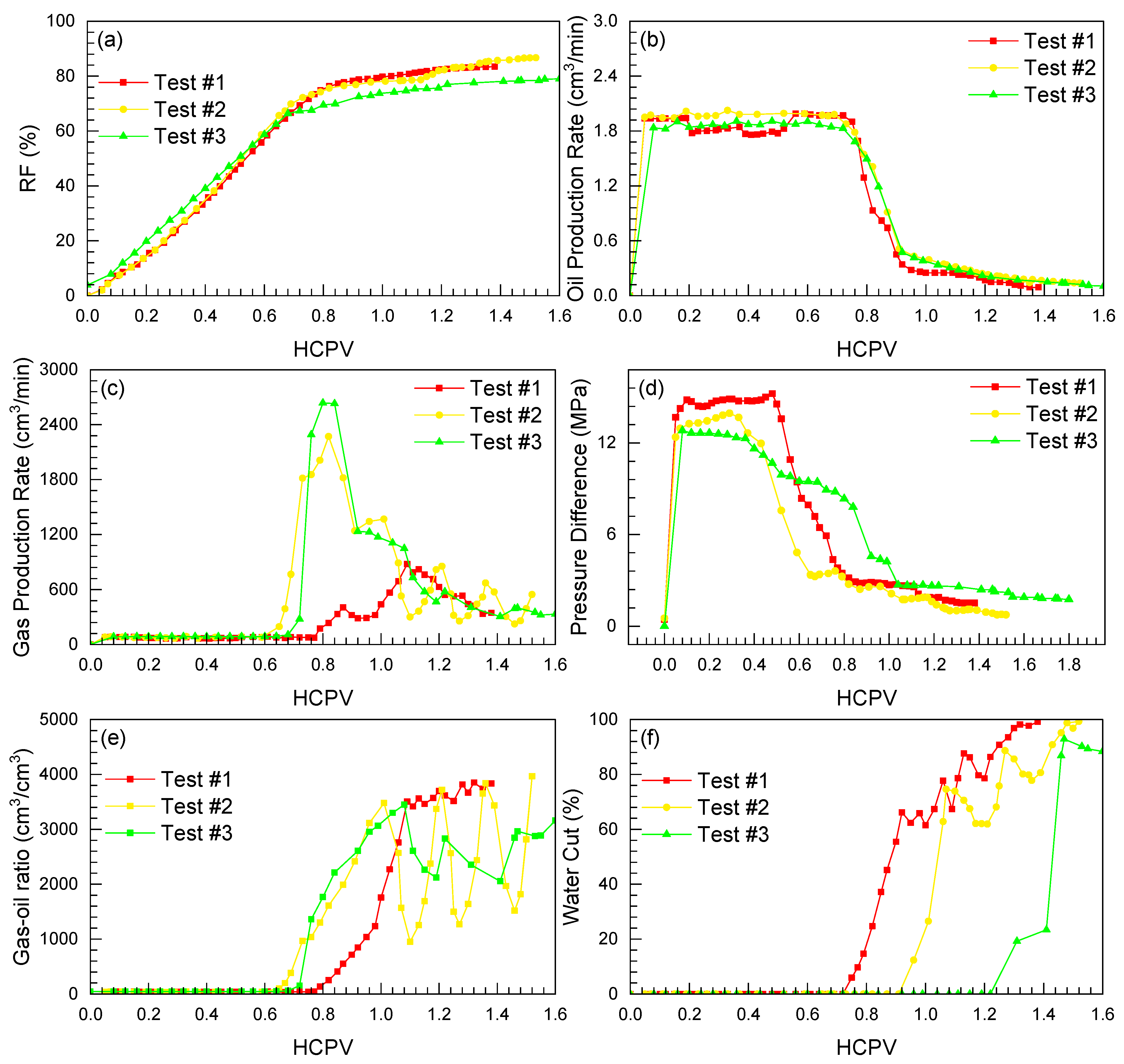
3.1. Results of the Homogeneous Core Displacement Experiment

Consider three different timing scenarios for the WAG intervention and conduct three sets of homogeneous core CO₂ displacement experiments. The production performance of the cores during these experiments is summarized in Table 4. The total injected hydrocarbon pore volume (HCPV) during the core displacement experiments includes the gas and water injections.

Upon comparing the results of the three core displacement experiments, it is evident that direct WAG injection outperforms WAG injection after gas breakthrough or complete gas channeling in terms of gas breakthrough at the outlet. The direct WAG injection achieves a high recovery factor of 74.82% (Table 4). In the subsequent WAG stage, direct WAG injection leads to a quicker water breakthrough, with an injection ratio (HCPV) of 0.75 (0.45 water + 0.3 CO₂) at the point of water breakthrough, and an associated recovery factor of 71.72%. From water breakthrough until the end of the displacement, the recovery factor improves from 71.72% to 83.38%, exhibiting an enhancement of 11.66%. In the case of WAG injection after gas breakthrough and WAG injection after complete gas channeling, the injection ratios (HCPV) at water breakthrough are 0.96 and 1.31, respectively. Upon comparing these two scenarios, it is evident that direct WAG injection performs slightly better in the pre-water breakthrough stage as compared to WAG injection after gas breakthrough or complete gas channeling. However, introducing WAG injection too early results in premature water breakthrough, subsequently reducing the magnitude of the recovery factor increase.

Figure 6a shows that there is no significant difference between direct WAG injection and WAG injection after gas breakthrough. However, the curve of WAG injection after complete gas channeling exhibits a lower recovery factor in the later stage. From Figure 6b,c, it can be seen that the gas–oil ratio and water cut increase rapidly after gas breakthrough and water breakthrough at the outlet of WAG drive. Additionally, with the gas–oil ratio and water content showing a wave-like high-level oscillation. Gas–oil ratio typically exceeds 1000 m³/m³, and water saturation surpasses 80%. Conversely, WAG injection after complete gas channeling demonstrates fewer fluctuations in gas–oil ratio and water saturation, whereas direct WAG injection demonstrates a gradual increase in gas–oil ratio. Figure 6d illustrates that direct WAG injection sustains a prolonged high displacement pressure differential time. Conversely, The displacement pressure difference of WAG flooding after gas breakthrough or WAG flooding after complete gas channeling decreases step by step with gas breakthrough and water breakthrough at the outlet end.

In summary, the curves demonstrate the effectiveness of WAG injection for homogeneous cores, with optimization depending on the timing of water injection. The main key node is when to intervene in the water phase.

3.2. Results of the Heterogeneous Core Displacement Experiment

Three sets of heterogeneous core CO₂ displacement experiments were conducted, considering three different timings for WAG intervention. Table 5 presents a summary of the production performance of the cores in these experiments. The injected HCPV during the core displacement experiments represents the total injection of gas and water into the cores.

The results of three core displacement experiments are compared. When the gas is found at the outlet, the direct WAG flooding is better than the WAG flooding after the gas is found or the gas is completely channeled. The oil recovery degree can reach up to 64.97% (Table 5). The injected HCPV is 0.53 (0.30 water + 0.23 CO₂) for direct WAG displacement, 0.79 (0.14 water + 0.65 CO₂) for WAG displacement after gas breakthrough, and 1.21 (0.22 water + 0.99 CO₂) for WAG displacement after complete gas channeling when water appears. It is worth noting that early introduction of WAG displacement leads to early water breakthrough; however, it effectively delays the gas channeling time and significantly improves the gas displacement efficiency.

The degree of oil recovery in direct WAG displacement increases gradually, whereas in WAG displacement after gas breakthrough and WAG displacement after complete gas channeling, it shows a step-like increase (Figure 7a). Figure 7b,c demonstrate that WAG displacement after gas breakthrough and WAG displacement after complete gas channeling result in a rapid increase in gas–oil ratio and water cut at the outlet. This increase is accompanied by a wave-like high-level oscillation of the gas–oil ratio and water cut, with the gas–oil ratio surpassing 2000 m³/m³ and water cut exceeding 80%. In contrast, direct WAG displacement exhibits a slow increase in the gas–oil ratio. Figure 7d illustrates that direct WAG flooding maintains a long time at high displacement pressure difference. However, the displacement pressure difference of WAG flooding after gas breakthrough or WAG flooding after complete gas channeling decreases step by step with gas breakthrough and water breakthrough at the outlet end.

It is evident from the entire curve that the earlier the heterogeneous core intervenes in the water phase, the better the effect of inhibiting gas channeling displacement.

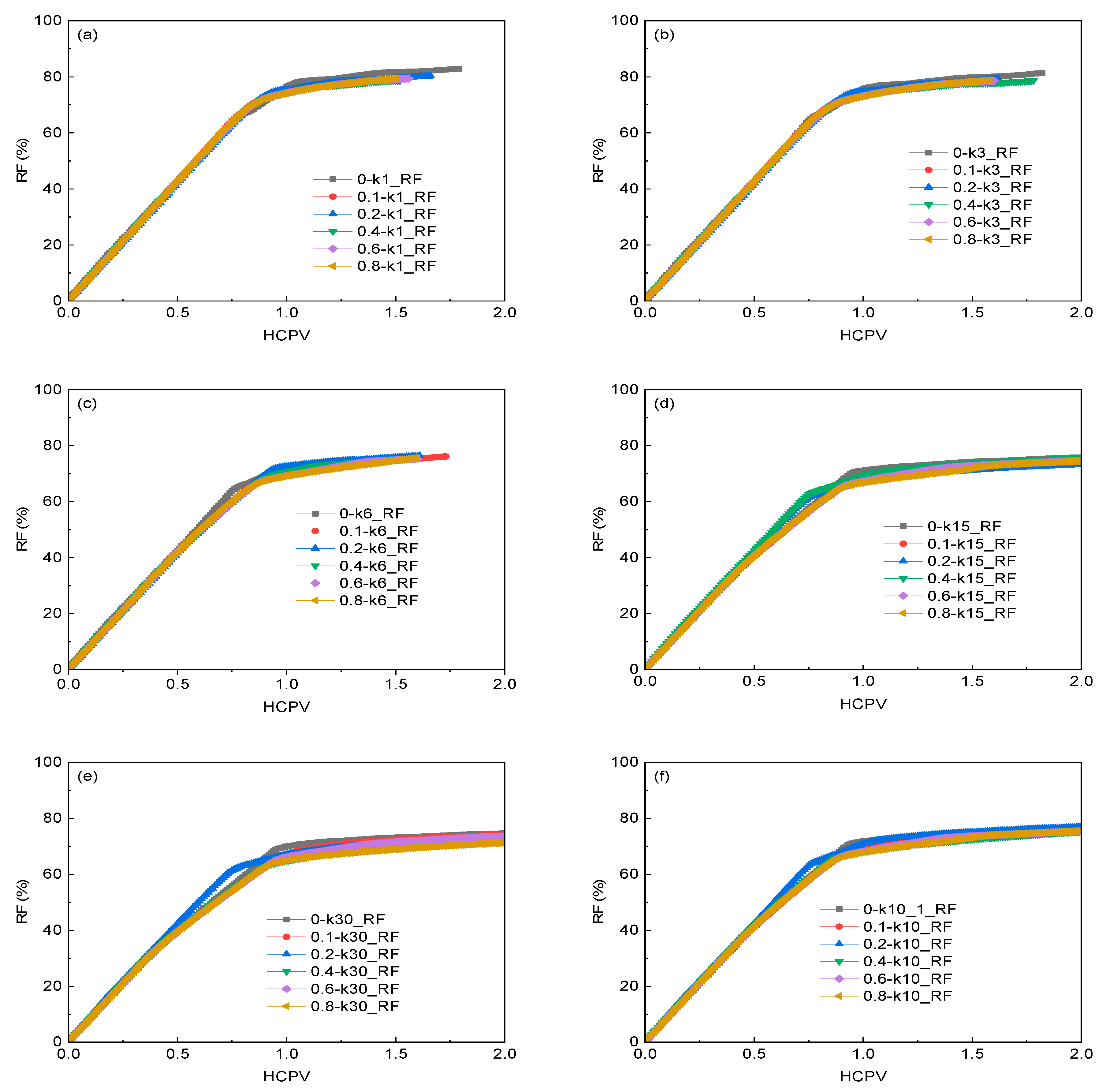
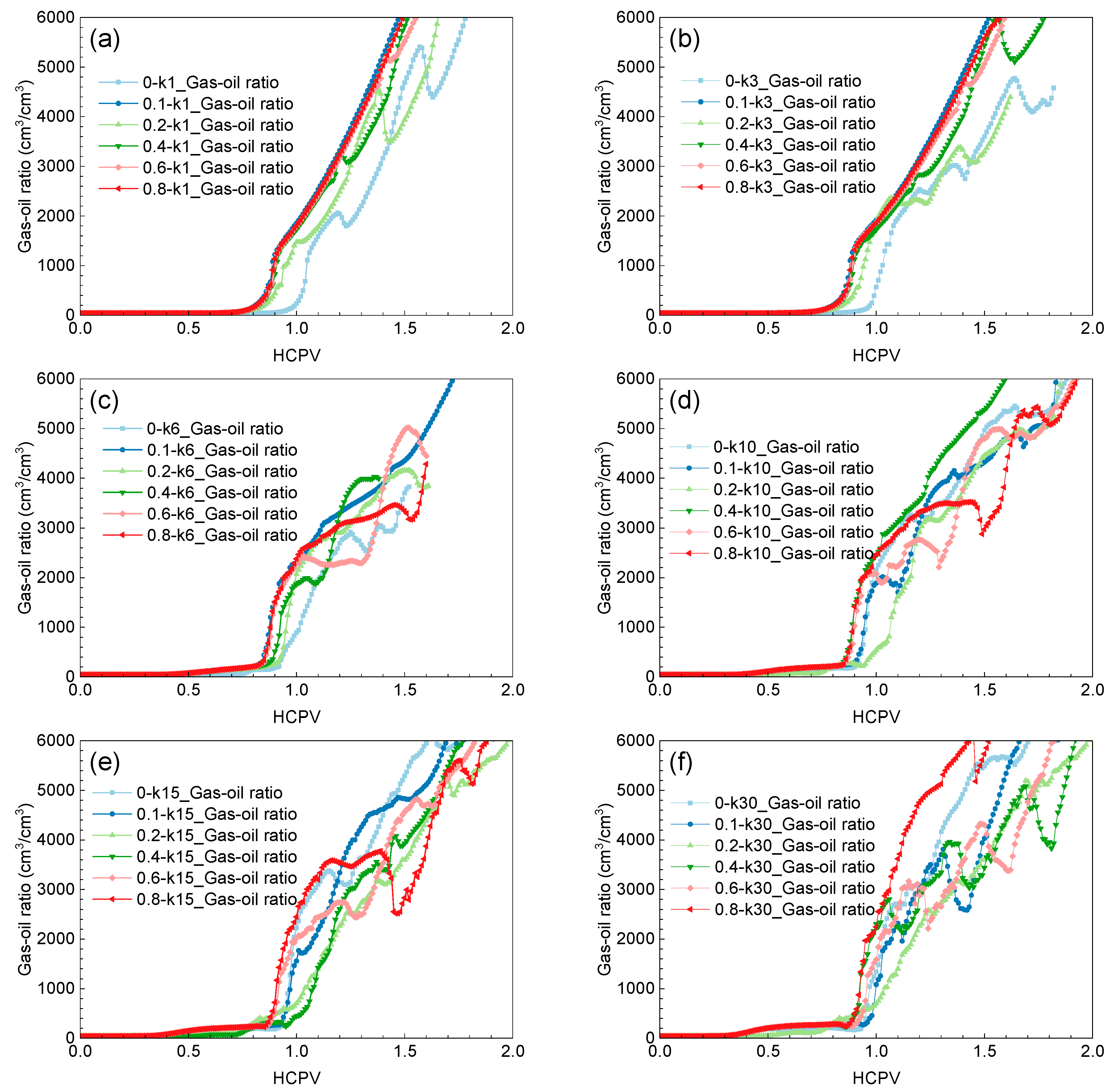
4. Pattern of Variation in WAG Intervention Timing

4.1. Numerical Simulation Modelling

Prior to history matching, characteristics of the light oil–CO₂ system were aligned utilizing the PVTi module (Version 2014) developed by Computer Modelling Group Ltd. (Schlumberger, Houston, TX, USA). Following this, the most harmonized model was applied in the E300 module (Schlumberger, Version 2014) to facilitate history matching of the CO₂ flooding experiments.

Numerical simulation studies were conducted to enhance understanding of the CO₂ flooding mechanism in low-permeability oil reservoirs and to align with experimental results. Experimental fitting was performed to assess the phase behavior of the reservoir oil–CO₂ system before history matching. Then, history matching was carried out for the CO₂ flooding experiment.

The parameters of the rock cores are presented in Table 2. The model possesses the same properties as the tested rock cores, including dimensions, permeability, and porosity. The model’s initial conditions are consistent with the reservoir’s initial conditions, with a temperature of 90 °C and a pressure of 20 MPa.

For precise simulation of the cylindrical physical model (core) illustrated in Figure 8, a grid system was established with 30 grids along the i-direction and 36 grids in the cross-sectional plane. Table 6 provides detailed information on grid dimensions and associated core parameters.

4.1.1. Oil Properties Study

To enhance understanding of the CO₂ flooding mechanism in low-permeability oil reservoirs and develop an accurate numerical model, the phase behavior of the oil–CO₂ system in the reservoir was modeled by fitting the experimental oil properties. To ensure computational accuracy and efficiency, this study divided the oil components into nine pseudo-components. Figure 9 presents the final segmentation results and molar composition of the pseudo-components, while the detailed composition of the components is available in Appendix A Table A2. Table 7 provides a list of measured and simulated oil properties, including viscosity, density, gas–oil ratio, saturation pressure, and volume coefficients. Figure 10 displays the measured and simulated properties of the oil–CO₂ system, while the detailed measurement errors can be found in Appendix A Table A3.

The measured and simulated minimum miscibility pressure (MMP) values, as demonstrated in Appendix A Figure A1, are 19.1 MPa and 18.3 MPa, respectively, with an error of 4.37%. Thus, the division of pseudo-components is justified, and the matching results between oil properties and oil–CO₂ system properties can be utilized for studying the CO₂ flooding process in low-permeability oil reservoirs.

4.1.2. Numerical Simulation Study

The primary factors influencing fluid flow in the model comprise the equation of state, relative permeability curves, and grid discretization. In the preceding section, the Peng–Robinson equation was employed to simulate the fluid’s phase behavior and property variations throughout the CO₂ flooding process. Figure 11 depicts the relative permeability curves following history matching. The grid properties, including porosity and permeability, are determined according to the distribution of properties presented in Table 2.

The simulation results exhibit a favorable agreement between the production data during the CO₂ flooding process and the historical dataset, as depicted in Figure 12 and Figure 13.

4.2. Characteristics of Displacement Front Changes

Figure 14a,b depict the variation in saturation profiles between interfacial WAG and direct WAG displacements following gas breakthrough in homogeneous rock cores. The gas front in the homogeneous rock cores exhibits a relatively uniform distribution without obvious breakthrough. Figure 14c,d illustrate the variations in saturation profiles between interfacial WAG and direct WAG displacements after gas breakthrough in heterogeneous rock cores. The influence of rock heterogeneity is evident as it causes uneven gas distribution, while WAG displacement retards the CO₂ migration rate, facilitating its complete dissolution into the oil and resulting in a more uniform gas front.

Before the gas displacement front reaches the outlet end, the gas front extends approximately 8.8 cm for WAG displacement and approximately 6.4 cm for direct WAG displacement (Figure 15). In the WAG method, injecting relatively high viscosity water prior to low viscosity CO₂ injection suppresses CO₂ channeling in high-permeability regions, leading to a more uniform displacement front and expanding the area influenced by gas displacement. Heterogeneous permeability creates channeling paths between injection and production wells, resulting in notable displacement front variations among different channels. Figure 15 illustrates that the inclination angles of the displacement front in high-permeability regions are approximately 72.30° for continuous gas displacement and 55.33° for direct WAG displacement, whereas in low-permeability regions, the angles are approximately 36.78° and 79.13°, respectively. During WAG displacement, water selectively enters high-permeability regions to stabilize the gas front, thus slowing down CO₂ migration and promoting enhanced gas injection into low-permeability regions, ultimately enlarging the area affected by gas displacement.

4.3. WAG Intervention Timing and Heterogeneous Relationships

The timing of WAG injection in relation to permeability heterogeneity was analyzed based on the historical fitting of the rock core size model. The study examined the optimal timing of WAG injection under varying levels of permeability heterogeneity. The design scheme is presented in Table 8.

Based on the results presented in Figure 16, as the degree of permeability heterogeneity increases, it is advisable to intervene earlier in the timing of WAG injection. For a detailed comparison curve, please refer to Figure A2, Figure A3 and Figure A4.

In reservoirs with lower heterogeneity, the differences in fluid distribution between high-permeability layers and low-permeability layers are insignificant. Although CO₂ is more likely to penetrate high-permeability layers, the disparity with low-permeability layers remains negligible. Therefore, introducing WAG injection before the occurrence of gas channeling is feasible; however, caution should be exercised to avoid intervening too early. Typically, when the permeability contrast is below 15, conducting WAG injection after observing gas breakthrough proves to be more effective.

In reservoirs characterized by higher heterogeneity, significant differences exist in reservoir properties between high-permeability layers and low-permeability layers. Gas has a tendency to preferentially flow through layers with higher permeability, leading to flow instability. Consequently, determining the optimal timing for WAG injection necessitates a profound comprehension of the fluid distribution and migration patterns within each layer. As Figure 17 demonstrates, a direct WAG drive is particularly effective when the permeability differential exceeds 15, especially in mitigating gas channeling. This strategy is notably more efficacious than introducing WAG drive after detecting gas channeling.

5. Upscaling Prediction Study

Utilizing a calibrated phase behavior model, the present study aimed to optimize the timing of CO₂ flooding in the target reservoir through the implementation of the WAG technique. Initially, the production process was simulated, followed by a rigorous fitting of the historical production dynamics. Subsequently, the timing of WAG injection was methodically optimized.

The permeability distribution of two well groups is presented in Figure 18. Figure 18a illustrates a well group exhibiting relatively good homogeneity, with a permeability contrast of 15. Figure 18b depicts a well group characterized by relatively poor heterogeneity, with a permeability contrast of 30. The historical matching curves for these actual well groups are displayed in Figure 19. The injection timing of WAG was optimized for each individual well group, as indicated in Table 9.

The cumulative oil production at different injection timings of WAG in two well groups is depicted in Figure 20. Figure 20a represents a well group characterized by a permeability contrast of 15. The cumulative oil production initially increases and then decreases with a delay in injection timing. The optimal effect of WAG injection is achieved after continuous gas injection for 1 year, with an accumulated injected hydrocarbon pore volume (HCPV) of approximately 0.12 times the HCPV. The cumulative oil production at this point is 8.32 × 10⁴ t, which exceeds that of direct WAG injection by 0.13 × 10⁴ t and exceeds that of WAG injection after 6 years by 0.96 × 10⁴ t. Figure 20b represents a well group characterized by a permeability contrast of 30. The cumulative oil production gradually decreases as the injection timing is delayed. The earlier the WAG injection is introduced, the more pronounced the injection effect becomes. Direct WAG injection yields the optimal result, with a cumulative oil production of 4.52 × 10⁴ t, surpassing that of WAG injection after gas breakthrough by 0.12 × 10⁴ t and surpassing that of WAG injection after 6 years by 0.77 × 10⁴ t.

6. Conclusions

This study conducts experiments to displace CO₂ on both homogeneous and heterogeneous rock cores, aiming to verify the correlation between the timing of WAG intervention and the level of heterogeneity. It optimizes the timing of WAG intervention under different heterogeneous conditions through experiments and numerical simulations, and also carries out field applications.

(1): The results of the experiment indicate a notable enhancement in oil recovery rate with WAG intervention in contrast to continuous CO₂ flooding. Nonetheless, the precise moment of WAG application is intricately linked to the degree of heterogeneity within the rock cores. In the case of homogeneous rock cores, the deployment of WAG post gas breakthrough results in a 5% elevated improvement in the recovery rate as opposed to its deployment following a complete gas sweep. Conversely, the immediate application of WAG in heterogeneous rock cores leads to a 4.83% increment in recovery rate compared to its deployment after a complete gas sweep.
(2): Due to the influence of rock heterogeneity, the gas front distribution during gas flooding exhibits nonlinear behavior. Upon injection of WAG, water initially infiltrates high-permeability zones, stabilizing the position of the gas front. Consequently, by slowing down CO₂ migration, it primarily guides the injected gas towards low-permeability zones, consequently increasing the extent of gas flooding. However, due to the influence of CO₂ distribution, there is an optimal time window for the full action of the aqueous phase, and this window has a significant relationship with the degree of heterogeneity.
(3): With increasing heterogeneity, early intervention with WAG flooding is preferable. When the permeability difference is less than 15, there is no significant variation in CO₂ interaction within the high-permeability and low-permeability layers. Timely intervention with WAG flooding is necessary before gas breakthrough occurs, but it should not occur too early. WAG flooding after gas breakthrough is more efficient. Reservoirs with a permeability contrast greater than 15 exhibit significant differences in the properties of the high-permeability and low-permeability layers. Gas tends to flow preferentially through the high-permeability layers, potentially causing flow instability. Direct WAG flooding is more efficient, especially in the control of gas channeling, which is better than the introduction of WAG drive after gas channeling is observed.
(4): By clarifying the matching relationship between the timing of WAG flooding and heterogeneity, more injected gas can be directed into low-permeability zones, increasing the sweep volume for oil recovery. This effectively reduces ineffective gas displacement and improves oil recovery efficiency. It also reduces the environmental risks associated with gas breakthrough, providing a more accurate basis for reservoir managers to formulate more scientific development strategies and operational parameters.

Author Contributions

Conceptualization, L.Z. and T.L.; methodology, Y.Y.; software, J.S.; validation, L.Z., T.L. and Y.Y.; formal analysis, L.Z. and G.S.; investigation, J.D.; resources, J.S.; data curation, J.D.; writing—original draft preparation, L.Z.; writing—review and editing, L.Z. and G.S.; visualization, J.S.; supervision, Y.Y.; project administration, T.L.; funding acquisition, T.L. All authors have read and agreed to the published version of the manuscript.

Funding

This research was funded by the Key Technology Project of China Petroleum & Chemical Corporation (SINOPEC) (No. P18088-2).

Data Availability Statement

Data sharing not applicable.

Acknowledgments

The author acknowledges the financial support provided by the Exploration and Development Research Institute of Shengli Oilfield Branch Company, China Petroleum & Chemical Corporation. The author also expresses appreciation to the reviewers and editors for their valuable feedback, which greatly contributed to the improvement of the manuscript.

Conflicts of Interest

The authors declare no conflict of interest.

Appendix A

Table A1. Table Compositional analysis results of the oil sample under the reservoir conditions (20 MPa, 90 °C).

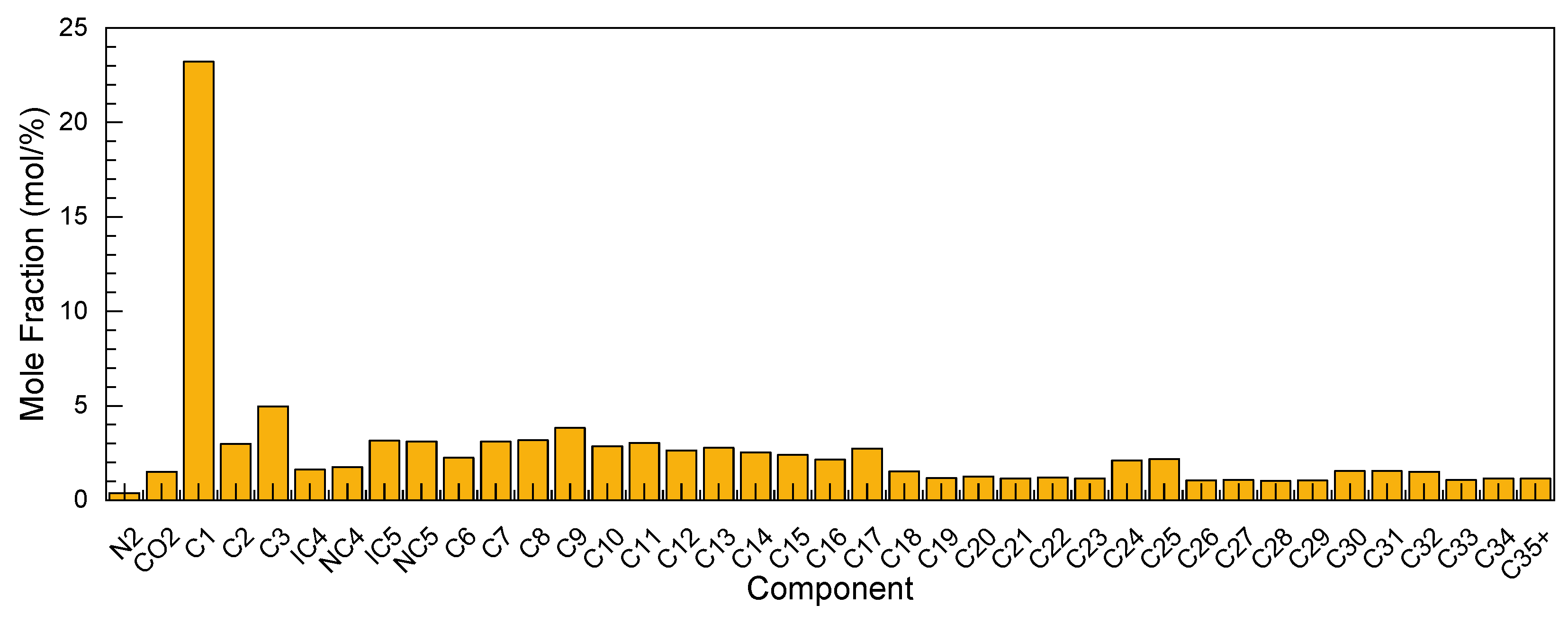
Carbon No.	mol/%	Wt (%)	Carbon No.	mol/%	Wt (%)
N₂	0.383	0.070	C17	2.736	4.215
CO₂	1.508	0.432	C18	1.529	2.494
C1	23.213	2.421	C19	1.162	1.986
C2	2.984	0.583	C20	1.252	2.238
C3	4.964	1.423	C21	1.158	2.191
IC4	1.620	0.612	C22	1.213	2.404
NC4	1.758	0.664	C23	1.158	2.394
IC5	3.150	1.477	C24	2.109	4.538
NC5	3.108	1.457	C25	2.173	4.873
C6	2.241	1.223	C26	1.055	2.462
C7	3.097	1.932	C27	1.075	2.612
C8	3.171	2.205	C28	1.011	2.548
C9	3.831	3.013	C29	1.040	2.718
C10	2.864	2.495	C30	1.536	4.153
C11	3.032	2.897	C31	1.536	4.292
C12	2.637	2.760	C32	1.506	4.347
C13	2.765	3.146	C33	1.062	3.163
C14	2.534	3.129	C34	1.145	3.511
C15	2.396	3.208	C35+	1.143	4.613
C16	2.149	3.101	Total	100.000	100.000

Table A2. Partition result and mole content of the pseudo-components.

Pseudo-Component	mol/%	Wt (%)
CO₂	1.51	0.43
C1+	23.60	2.47
C2+	7.95	2.04
C4+	9.63	4.19
C6+	12.34	8.39
C10+	13.83	14.42
C15+	11.22	17.14
C22+	7.81	16.21
C27+	12.11	34.72

Table A3. Characteristics of the oil–CO₂ system at different CO₂ concentrations under different pressures.

C_CO2	Saturation Pressure (MPa)			Oil Density (kg/m³)			Oil Viscosity (mPa·s)			Oil Swelling Factor (m³/m³)
C_CO2	MD	SD	Error	MD	SD	Error	MD	SD	Error	MD	SD	Error
0	10.8	10.8	0	766.3	778.7	1.62	2.02	2.12	4.95	1	1	0
29.5	15.79	15.01	4.94	747.1	755.3	1.1	1.52	1.54	1.32	1.03	1.02	0.97
46.5	20.51	21.02	2.49	746.3	736.1	1.37	1.19	1.14	4.2	1.08	1.06	1.85
57	26.15	25.2	3.63	729.4	727.4	0.27	1	0.92	8	1.15	1.11	3.48
63.7	29.67	28.72	3.2	719.4	722.7	0.46	0.92	0.83	9.78	1.24	1.25	0.81
67.6	33.66	32.32	3.98	709.7	720.4	1.51	0.85	0.78	8.24	1.62	1.52	6.17

Note: C_CO2 = concentration of CO₂ in light oil–CO₂ systems; MD = measured data; SD = simulation data.

Figure A1. Measured and simulated MMP for the live oil.

Figure A2. Comparison of recovery factor at different WAG intervention times under different permeability contrast: (a) Permeability contrast 1; (b) Permeability contrast 3; (c) Permeability contrast 6; (d) Permeability contrast 10; (e) Permeability contrast 15; (f) Permeability contrast 30.

Figure A3. Comparison of Gas–Oil Ratios at Different WAG Intervention Times Under Different Permeability contrast: (a) Permeability contrast 1; (b) Permeability contrast 3; (c) Permeability contrast 6; (d) Permeability contrast 10; (e) Permeability contrast 15; (f) Permeability contrast 30.

Figure A4. Comparison of water cut at different WAG intervention times under different permeability contrast: (a) Permeability contrast 1; (b) Permeability contrast 3; (c) Permeability contrast 6; (d) Permeability contrast 10; (e) Permeability contrast 15; (f) Permeability contrast 30.

References

Kang, W.L.; Zhou, B.B.; Issakhov, M.; Gabdullin, M. Advances in enhanced oil recovery technologies for low permeability reservoirs. Pet. Sci. 2022, 19, 1622–1640. [Google Scholar] [CrossRef]
Liu, Z.-X.; Liang, Y.; Wang, Q.; Guo, Y.-J.; Gao, M.; Wang, Z.-B.; Liu, W.-L. Status and progress of worldwide EOR field applications. J. Pet. Sci. Eng. 2020, 193, 107449. [Google Scholar] [CrossRef]
Liu, Z.-X.; Gao, M.; Zhang, X.-M.; Liang, Y.; Guo, Y.-J.; Liu, W.-L.; Bao, J.-W. CCUS and CO₂ injection field application in abroad and China: Status and progress. Geoenergy Sci. Eng. 2023, 229, 212011. [Google Scholar] [CrossRef]
Song, Z.; Song, Y.; Li, Y.; Bai, B.; Song, K.; Hou, J. A critical review of CO₂ enhanced oil recovery in tight oil reservoirs of North America and China. Fuel 2020, 276, 118006. [Google Scholar] [CrossRef]
Kulkarni, M.M.; Rao, D.N. Experimental investigation of miscible and immiscible Water-Alternating-Gas (WAG) process performance. J. Pet. Sci. Eng. 2005, 48, 1–20. [Google Scholar] [CrossRef]
Liu, S.-Y.; Ren, B.; Li, H.-Y.; Yang, Y.-Z.; Wang, Z.-Q.; Wang, B.; Xu, J.-C.; Agarwal, R. CO₂ storage with enhanced gas recovery (CSEGR): A review of experimental and numerical studies. Pet. Sci. 2022, 19, 594–607. [Google Scholar] [CrossRef]
Kamali, F.; Hussain, F.; Cinar, Y. An experimental and numerical analysis of water-alternating-gas and simultaneous-water-and-gas displacements for carbon dioxide enhanced oil recovery and storage. SPE J. 2017, 22, 521–538. [Google Scholar] [CrossRef]
Wang, Y.-Y.; Wang, X.-G.; Dong, R.-C.; Teng, W.-C.; Zhan, S.-Y.; Zeng, G.-Y.; Jia, C.-Q. Reservoir heterogeneity controls of CO₂-EOR and storage potentials in residual oil zones: Insights from numerical simulations. Petrol. Sci. 2023. [Google Scholar] [CrossRef]
Diwu, P.; Liu, T.; You, Z.; Hou, G.; Qiao, R.; Zhao, L. Study on pulse characteristic of produced crude composition in CO₂ Flooding Pilot Test. Geofluids 2018, 2018, 1–5. [Google Scholar] [CrossRef]
Zhao, K.; Jia, C.; Li, Z.; Du, X.; Wang, Y.; Li, J.; Yao, Z.; Yao, J. Recent Advances and Future Perspectives in Carbon Capture, Transportation, Utilization, and Storage (CCTUS) Technologies: A Comprehensive Review. Fuel 2023, 351, 128913. [Google Scholar] [CrossRef]
Jafarian, K.; Kayhani, M.; Nazari, M.; Ghorbanbakhsh, B.; Shokri, N. WAG injection in porous media: A microfluidic analysis. Chem. Eng. Res. Des. 2023, 193, 649–659. [Google Scholar] [CrossRef]
Christensen, J.R.; Stenby, E.H.; Skauge, A. Review of WAG field experience. SPE Reserv. Eval. Eng. 2001, 4, 97–106. [Google Scholar] [CrossRef]
Kumar, N.; Sampaio, M.A.; Ojha, K.; Hoteit, H.; Mandal, A. Fundamental aspects, mechanisms and emerging possibilities of CO₂ miscible flooding in enhanced oil recovery: A review. Fuel 2022, 330, 125633. [Google Scholar] [CrossRef]
Pal, M. Water alternating gas (WAG) recovery process evaluation through simulation for a giant middle-eastern carbonate reservoir. Pet. Sci. Technol. 2022, 40, 1233–1257. [Google Scholar] [CrossRef]
Wang, Y.-F.; Li, Z.-Y.; Zhang, S.-M.; Liu, D.-X.; Ding, M.-C. Remaining oil distribution in models with different heterogeneities after CO₂ WAG injection: Visual research by nuclear magnetic resonance technique. J. Cent. South Univ. (Engl. Ed.) 2021, 28, 1412–1421. [Google Scholar] [CrossRef]
Hou, G.; Yang, Y.; Wang, W.; Cai, G.; Liu, T.; Hou, J. Theoretical design study of gas-water ratio during CO₂ flooding with variable cycle water alternating gas in low permeability reservoirs. Sci. Technol. Eng. 2020, 20, 6857–6864. [Google Scholar]
Scerbacova, A.; Mukhina, E.; Bakulin, D.; Burukhin, A.; Ivanova, A.; Cheremisin, A.; Spivakova, M.; Ushakova, A.; Cheremisin, A. Water-and Surfactant-Based Huff-n-Puff Injection into Unconventional Liquid Hydrocarbon Reservoirs: Experimental and Modeling Study. Energy Fuels 2023, 37, 11067–11082. [Google Scholar] [CrossRef]
Bello, A.; Ivanova, A.; Rodionov, A.; Aminev, T.; Mishin, A.; Bakulin, D.; Grishin, P.; Belovus, P.; Penigin, A.; Kyzyma, K.; et al. An Experimental Study of High-Pressure Microscopy and Enhanced Oil Recovery with Nanoparticle-Stabilised Foams in Carbonate Oil Reservoir. Energies 2023, 16, 5120. [Google Scholar] [CrossRef]
Yu, H.; Fu, W.; Zhang, Y.; Lu, X.; Cheng, S.; Xie, Q.; Qu, X.; Yang, W.; Lu, J. Experimental study on EOR performance of CO₂-based flooding methods on tight oil. Fuel 2021, 290, 119988. [Google Scholar] [CrossRef]
Chowdhury, S.; Rakesh, M.; Medhi, S.; Shrivastava, S.; Dehury, R.; Sangwai, J.S. Three-phase fluid flow interaction at pore scale during water- and surfactant-alternating gas (WAG/SAG) injection using carbon dioxide for geo-sequestration and enhanced oil recovery. Energy Fuels 2023, 37, 5270–5290. [Google Scholar] [CrossRef]
Wang, L.; He, Y.; Wang, Q.; Liu, M.; Jin, X. Multiphase flow characteristics and EOR mechanism of immiscible CO₂ water-alternating-gas injection after continuous CO₂ injection: A micro-scale visual investigation. Fuel 2020, 282, 118689. [Google Scholar] [CrossRef]
Song, X.; Wang, F.; Ma, D.; Gao, M.; Zhang, Y. Progress and prospect of carbon dioxide capture, utilization and storage in CNPC oilfields. Pet. Explor. Dev. 2023, 50, 229–244. [Google Scholar] [CrossRef]
Zhang, Y.; Zou, Y.; Zhang, Y.; Wang, L.; Liu, D.; Sun, J.; Ge, H.; Zhou, D. Experimental study on characteristics and mechanisms of matrix pressure transmission near the fracture surface during post-fracturing shut-in in tight oil reservoirs. J. Pet. Sci. Eng. 2022, 219, 111133. [Google Scholar] [CrossRef]
Olalotiti-Lawal, F.; Onishi, T.; Datta-Gupta, A.; Fujita, Y.; Watanabe, D.; Hagiwara, K. Model calibration and optimization of a post-combustion CO₂ WAG pilot in a mature oil field. Fuel 2019, 255, 115810. [Google Scholar] [CrossRef]
Ren, D.; Wang, X.; Kou, Z.; Wang, S.; Wang, H.; Wang, X.; Tang, Y.; Jiao, Z.; Zhou, D.; Zhang, R. Feasibility evaluation of CO₂ EOR and storage in tight oil reservoirs: A demonstration project in the Ordos Basin. Fuel 2023, 331, 125652. [Google Scholar] [CrossRef]
Han, J.; Lee, M.; Lee, W.; Lee, Y.; Sung, W. Effect of gravity segregation on CO₂ sequestration and oil production during CO₂ flooding. Appl. Energy 2016, 161, 85–91. [Google Scholar] [CrossRef]
Zhou, X.; Yuan, Q.; Rui, Z.; Wang, H.; Feng, J.; Zhang, L.; Zeng, F. Feasibility study of CO₂ huff “n” puff process to enhance heavy oil recovery via long core experiments. Appl. Energy. 2019, 236, 526–539. [Google Scholar] [CrossRef]
Hao, Y.; Li, Z.; Su, Y.; Kong, C.; Chen, H.; Meng, Y. Experimental investigation of CO₂ storage and oil production of different CO₂ injection methods at pore-scale and core-scale. Energy 2022, 254, 124349. [Google Scholar] [CrossRef]
Liu, T.; Diwu, P.; Jiang, B.; Jiang, L.; Liu, R. Theoretical simulation study on controlling factors in horizontal well CO₂ stimulation of heavy oil. Adv. Mech. Eng. 2014, 6, 695042. [Google Scholar] [CrossRef]
Hou, G.; Liu, T.; Yuan, X.; Hou, J.; Diwu, P. Study on the variation rule of produced oil components during CO₂ flooding in low permeability reservoirs. Comput. Model. Eng. 2020, 123, 1223–1246. [Google Scholar] [CrossRef]
Vásquez Haro, H.A.; de Gomes, M.S.P.; Rodrigues, L.G. Numerical analysis of carbon dioxide injection into a high permeability layer for CO₂-EOR projects. J. Pet. Sci. Eng. 2018, 171, 164–174. [Google Scholar] [CrossRef]
Kumar, S.; Mandal, A. A comprehensive review on chemically enhanced water alternating gas/CO₂ (CEWAG) injection for enhanced oil recovery. J. Pet. Sci. Eng. 2017, 157, 696–715. [Google Scholar] [CrossRef]
Tan, Y.; Li, Q.; Xu, L.; Ghaffar, A.; Zhou, X.; Li, P. A critical review of carbon dioxide enhanced oil recovery in carbonate reservoirs. Fuel 2022, 328, 125256. [Google Scholar] [CrossRef]
Guo, Y.; Liu, F.; Qiu, J.; Xu, Z.; Bao, B. Microscopic transport and phase behaviors of CO₂ injection in heterogeneous formations using microfluidics. Energy 2022, 256, 124524. [Google Scholar] [CrossRef]
Wang, H.; Tian, L.; Huo, M.; Xu, S.; Liu, Z.; Zhang, K. Dynamic track model of miscible CO₂ geological utilizations with complex microscopic pore-throat structures. Fuel 2022, 322, 124192. [Google Scholar] [CrossRef]
Wang, Y.; Han, X.; Li, J.; Liu, R.; Wang, Q.; Huang, C.; Wang, X.; Zhang, L.; Lin, R. Review on oil displacement technologies of enhanced oil recovery: State-of-the-art and outlook. Energy Fuels 2023, 37, 2539–2568. [Google Scholar] [CrossRef]
Wang, H.; Kou, Z.; Ji, Z.; Wang, S.; Li, Y.; Jiao, Z.; Johnson, M.; McLaughlin, J.F. Investigation of enhanced CO₂ storage in deep saline aquifers by WAG and brine extraction in the Minnelusa sandstone, Wyoming. Energy 2023, 265, 126379. [Google Scholar] [CrossRef]
Menad, N.A.; Noureddine, Z. An efficient methodology for multi-objective optimization of water alternating CO₂ EOR process. J. Taiwan Inst. Chem. Eng. 2019, 99, 154–165. [Google Scholar] [CrossRef]
Seyyedi, M.; Mahzari, P.; Sohrabi, M. A fundamental micro scale study of the roles of associated gas content and different classes of hydrocarbons on the dominant oil recovery mechanism by CWI. Sci. Rep. 2019, 9, 5996. [Google Scholar] [CrossRef]

Figure 1. Schematic representation of the distribution of carbon dioxide (CO₂) and injected water in porous media with different levels of heterogeneity: (a) Gas displacement in a homogeneous medium results in a uniform displacement front; (b) gas displacement leads to a front that advances further in the larger pore throats in a heterogeneous medium: (c) injecting WAG results in a relatively uniform displacement front prior to displacement in a heterogeneous medium.

Figure 2. Compositional analysis results of the oil sample under the reservoir conditions (20 MPa, 90 °C).

Figure 3. Sample images of the layered cores: (a) homogeneity core; (b) heterogeneity core. ① Two artificial core plates, each with distinct permeabilities, underwent individual pressure tests. ② From one end of the core block, a cylindrical core plug of 3.6 centimeters in diameter was extracted. This plug comprises two segments, each with a permeability corresponding to a different layer of the core block. ③ To construct a 90-cm-high core column, three sets of core samples were combined.

Figure 4. Schematic of the experimental setup for the property tests of light oil–CO₂ systems: (a) viewing window designed for high-pressure and high-temperature conditions, with an inner diameter of 3.177 cm and an effective volume of 125.620 cm³; (b) DBR pump; (c) oil and gas separator (resolution: 0.1 cm³) and gas flow meter (resolution: ±0.2%); (d) density meter (resolution: 0.0001 g/cm³); (e) rolling ball viscometer (resolution: 0.1%).

Figure 5. Schematic diagram of the high-pressure CO₂ coreflood apparatus: (a) Pump that automatically displaces fluids; (b) Oven capable of maintaining a constant temperature of 90 °C for reservoir simulation; (c) Oven capable of maintaining ambient temperature; (d) Regulator used to control back pressure; (e) Digital gauge for measuring differential pressure; (f) Meter for measuring gas flow rate.

Figure 6. Experimental results of the CO₂ flooding process conducted on homogeneous cores: (a) oil recovery factor changes with HCPV for each experiment; (b) oil production rate changes with HCPV for each experiment; (c) gas production rate changes with HCPV for each experiment; (d) pressure difference (pressure at the inlet minus pressure at the outlet) changes with HCPV for each experiment; (e) gas–oil ratio (cm³ of gas prod/cm³ of oil prod) changes with HCPV for each experiment; (f) water cut changes with HCPV for each experiment.

Figure 7. Experimental results of the CO₂ flooding process: (a) oil recovery factor changes with HCPV for each experiment; (b) oil production rate changes with HCPV for each experiment; (c) gas production rate changes with HCPV for each experiment; (d) pressure difference (pressure at the inlet minus pressure at the outlet) changes with HCPV for each experiment; (e) gas–oil ratio (cm³ of gas prod/cm³ of oil) changes with HCPV for each experiment; (f) water cut changes with HCPV for each experiment.

Figure 8. Schematic diagram of the historical fitting model for CO₂ flooding process (permeability of the model is indicated in the diagram, unit: mD).

Figure 9. Partition result and mole content of the pseudo-components.

Figure 10. Characteristics of the oil–CO₂ system at different CO₂ concentrations under different pressures: (a) saturation pressure; (b) oil density; (c) oil viscosity; (d) oil swelling factor.

Figure 11. Relative permeability curves: (a) water and oil system; (b) oil and gas system.

Figure 12. Similarity Curve for Gas–Oil Production in Expulsion Replacement Experiments: (a) Fit curve for Test #1; (b) Fit curve for Test #2; (c) Fit curve for Test #3; (d) Fit curve for Test #4; (e) Fit curve for Test #5; (f) Fit curve for Test #6.

Figure 13. Similarity Curve for recovery factor in Expulsion Replacement Experiments: (a) Fit curve for Test #1; (b) Fit curve for Test #2; (c) Fit curve for Test #3; (d) Fit curve for Test #4; (e) Fit curve for Test #5; (f) Fit curve for Test #6.

Figure 14. Chart depicting the variation in oil saturation levels along the wellbore during core retrieval: (a) Test #2; (b) Test #1; (c) Test #5; (d) Test #4.

Figure 15. Heterogeneous Core Gas Drive Front Edge Schematic Diagram.

Figure 16. Comparative analysis of recovery rates corresponding to different permeability differentials and intervention timings (a) Permeability contrast 1; (b) Permeability contrast 3; (c) Permeability contrast 6; (d) Permeability contrast 10; (e) Permeability contrast 15; (f) Permeability contrast 30.

Figure 17. Relationship graph between WAG intervention timing and heterogeneity degree.

Figure 18. The actual distribution of block wells and the degree of heterogeneity in permeability: (a) Permeability contrast 15; (b) Permeability contrast 30.

Figure 19. Historical Matching Curves for Actual Well Groups: (a) Cumulative Liquid Production Curve for Well Group A; (b) Cumulative Oil Production Curve for Well Group A; (c) Cumulative Liquid Production Curve for Well Group B; (d) Cumulative Oil Production Curve for Well Group B.

Figure 20. Comparison Chart of Cumulative Oil Production at Different Stages of WAG Injection Timing Intervention: (a) Permeability contrast 15; (b) Permeability contrast 30.

Table 1. Measured properties for the studied light oil sample.

Parameter	Live Oil ¹
Crude oil density (kg/m³)	764.2
Crude oil viscosity (mPa·s)	1.04
Solution gas–oil ratio (GOR)(sm³/m³)	44
Saturation pressure (MPa)	8.95
Oil formation volume factor (m³/m³)	1.1647

¹ The properties of live oil were tested under reservoir conditions (20 MPa, 90 °C).

Table 2. Properties of the cores applied in this study.

Core No.	Length (cm)	Diameter (cm)	Permeability (mD)	Permeability Contrast	Average Porosity (%)
A	90	3.6	4.73	1	11.25
B	90	3.6	2.43, 8.60	3	9.10

Table 3. Design of the experiment.

Number	WAG Intervention	WAG Ratio	WAG Size	Pressure	Temperature
Test #1	Direct WAG drive	1:1	Injection of 0.1 HCPV water + 0.1 HCPV gas	20 MPa	90 °C
Test #2	Intervention of WAG drive after the outlet gas–oil ratio reaches 100 m³/m³
Test #3	Intervention of WAG drive when the outlet gas–oil ratio reaches 3000 m³/m³

Table 4. Production performances in homogeneous cores for the core-flooding experiments using different media.

Core Type	Experiment	GBT (w/g) ² (HCPV) ¹	RF_GBT ⁴ (%)	WBT (w/g) ³ (HCPV)	RF_WBT ⁵ (%)	Q_w ⁷ (HCPV)	Q_CO2 ⁸ (HCPV)	RF ⁶ (%)
A	Test #1	0.39/0.4	74.82	0.45/0.3	71.72	0.71	0.67	83.38
	Test #2	0/0.65	65.66	0.18/0.78	77.81	0.44	1.08	86.70
	Test #3	0/0.68	66.36	0.09/1.2	77.57	0.19	1.41	81.20

Note: Test #1: Direct WAG drive; Test #2: Intervention of WAG drive after the outlet gas–oil ratio reaches 100 m³/m³; Test #3: Intervention of WAG drive when the outlet gas–oil ratio reaches 3000 m³/m³. ¹ HCPV: hydrocarbon pore volume, cm³; ² GBT (w/g): gas breakthrough occurs at the water/gas injection volume, HCPV; ³ WBT (w/g): water breakthrough occurs at the water/gas injection volume, HCPV; ⁴ RF_GBT: gas breakthrough occurs at the oil recovery factor, %; ⁵ RF_WBT: water breakthrough occurs at the oil recovery factor, %; ⁶ RF: oil recovery factor, %; ⁷ Q_w: volume of water injection, HCPV; ⁸ Q_CO2: volume of CO₂ injection, HCPV.

Table 5. Production performances in heterogeneous cores for the core-flooding experiments using different media.

Core Type	Experiment	GBT (w/g) (HCPV)	RF_GBT (%)	WBT (w/g) (HCPV)	RF_WBT (%)	Q_w (HCPV)	Q_CO2 (HCPV)	RF (%)
B	Test #4	0.42/0.31	64.97	0.30/0.23	51.88	0.74	0.77	81.88
	Test #5	0/0.55	52.39	0.14/0.65	65.07	0.56	0.94	78.63
	Test #6	0/0.49	45.07	0.22/0.99	70.55	0.54	1.22	77.05

Note: Test #4: Direct WAG drive; Test #5: Intervention of WAG drive after the outlet gas–oil ratio reaches 100 m³/m³; Test #6: Intervention of WAG drive when the outlet gas–oil ratio reaches 3000 m³/m³.

Table 6. Basic reservoir parameters of the geological and petrophysical models.

Parameters	Values
Grid in x, y and z directions	30 × 6 × 6 = 1080
Grid size in x direction, cm	3
Grid size in y direction, cm	0.6
Average grid size in z direction, cm	0.6
Reservoir temperature, °C	90
Initial reservoir pressure, MPa	20

Table 7. Measured and simulated oil properties.

Parameters	MD	SD	Error (%)
Saturation pressure (MPa)	10.80	10.60	1.85
Crude oil density (kg/m³)	751.50	778.70	3.62
Crude oil viscosity (mPa·s)	2.02	2.12	4.89
Solution gas–oil ratio (GOR) (m³/m³)	48.10	49.60	3.12
Oil formation volume factor (m³/m³)	1.24	1.26	1.61

Note: MD = measured data; SD = simulation data.

Table 8. Model design framework for WAG timing interventions and heterogeneous relationships.

Factors that Affect	Levels of Parameters
Permeability contrast	1, 3, 6, 10, 15, 30
Timing of WAG intervention/injection of HCPV	0, 0.1, 0.2, 0.4, 0.6, 0.8

Table 9. Design table for WAG intervention timing in well group model.

No.	Timing of WAG Intervention
1	direct WAG drive
2	WAG drive intervention after 1 year of gas injection
3	WAG drive intervention after 2 year of gas injection
4	WAG drive intervention after 4 year of gas injection
5	WAG drive intervention after 6 year of gas injection

Disclaimer/Publisher’s Note: The statements, opinions and data contained in all publications are solely those of the individual author(s) and contributor(s) and not of MDPI and/or the editor(s). MDPI and/or the editor(s) disclaim responsibility for any injury to people or property resulting from any ideas, methods, instructions or products referred to in the content.

© 2023 by the authors. Licensee MDPI, Basel, Switzerland. This article is an open access article distributed under the terms and conditions of the Creative Commons Attribution (CC BY) license (https://creativecommons.org/licenses/by/4.0/).

Share and Cite

MDPI and ACS Style

Zhao, L.; Sang, G.; Ding, J.; Sun, J.; Liu, T.; Yao, Y. Research on the Timing of WAG Intervention in Low Permeability Reservoir CO₂ Flooding Process to Improve CO₂ Performance and Enhance Recovery. Energies 2023, 16, 7373. https://doi.org/10.3390/en16217373

AMA Style

Zhao L, Sang G, Ding J, Sun J, Liu T, Yao Y. Research on the Timing of WAG Intervention in Low Permeability Reservoir CO₂ Flooding Process to Improve CO₂ Performance and Enhance Recovery. Energies. 2023; 16(21):7373. https://doi.org/10.3390/en16217373

Chicago/Turabian Style

Zhao, Lekun, Guoqiang Sang, Jialei Ding, Jiangfei Sun, Tongjing Liu, and Yuedong Yao. 2023. "Research on the Timing of WAG Intervention in Low Permeability Reservoir CO₂ Flooding Process to Improve CO₂ Performance and Enhance Recovery" Energies 16, no. 21: 7373. https://doi.org/10.3390/en16217373

Note that from the first issue of 2016, this journal uses article numbers instead of page numbers. See further details here.

Article Menu

Research on the Timing of WAG Intervention in Low Permeability Reservoir CO₂ Flooding Process to Improve CO₂ Performance and Enhance Recovery

Abstract

1. Introduction