Article

Equipment- and Time-Constrained Data Acquisition Protocol for Non-Intrusive Appliance Load Monitoring

by
Konstantinos Koasidis
,
Vangelis Marinakis
,
Haris Doukas
,
Nikolaos Doumouras
,
Anastasios Karamaneas
and
Alexandros Nikas
*
Energy Policy Unit, School of Electrical and Computer Engineering, National Technical University of Athens, 15780 Athens, Greece
*
Author to whom correspondence should be addressed.
Energies 2023, 16(21), 7315; https://doi.org/10.3390/en16217315
Submission received: 12 September 2023 / Revised: 19 October 2023 / Accepted: 26 October 2023 / Published: 28 October 2023
(This article belongs to the Special Issue Energy Efficiency of the Buildings II)

Abstract

:
Energy behaviours will play a key role in decarbonising the building sector but require the provision of tailored insights to assist occupants to reduce their energy use. Energy disaggregation has been proposed to provide such information on the appliance level without needing a smart meter plugged in to each load. However, the use of public datasets with pre-collected data employed for energy disaggregation is associated with limitations regarding its compatibility with random households, while gathering data on the ground still requires extensive, and hitherto under-deployed, equipment and time commitments. Going beyond these two approaches, here, we propose a novel data acquisition protocol based on multiplexing appliances’ signals to create an artificial database for energy disaggregation implementations tailored to each household and dedicated to performing under conditions of time and equipment constraints, requiring that only one smart meter be used and for less than a day. In a case study of a Greek household, we train and compare four common algorithms based on the data gathered through this protocol and perform two tests: an out-of-sample test in the artificially multiplexed signal, and an external test to predict the household’s appliances’ operation based on the time series of a real total consumption signal. We find accurate monitoring of the operation and the power consumption level of high-power appliances, while in low-power appliances the operation is still found to be followed accurately but is also associated with some incorrect triggers. These insights attest to the efficacy of the protocol and its ability to produce meaningful tips for changing energy behaviours even under constraints, while in said conditions, we also find that long short-term memory neural networks consistently outperform all other algorithms, with decision trees closely following.

1. Introduction

Decarbonising buildings will be crucial in the fight against climate change, since the sector is associated with high amounts of energy consumed and emissions produced—both directly from the combustion of fossil fuels, mainly for heating, as well as indirectly through electricity consumption. The European Union (EU), as part of the European Green Deal, has set ambitious targets for the sector, aiming to reduce emissions by 60% in 2030 and achieve net zero emissions by 2050 in buildings. To achieve these, the European Commission (EC) has launched policies and initiatives as part of the EGD and the ‘fit for 55’ package [1], namely the recast of the Energy Efficiency Directive and the energy performance of buildings directive, alongside the renovation wave strategy as well as long-term renovation strategies at the member state level. These documents set goals for the rate of renovations as well as introducing mechanisms to assist towards improving the performance of the building stock. Notably, the building sector is also set to become part of the EU Emissions Trading System (ETS) through the ETS II initiative, expanding the conventional representation of sectors in the ETS road transport and buildings [2]. These targets and sectoral policies, in line with the broader European climate goals of reducing economy-wide greenhouse gas (GHG) emissions by 55% in 2030 and achieving a net zero European economy by 2050, will require a combination of energy efficiency interventions, demand-side electricity generation from renewable sources, as well as behavioural changes [3,4].
In this effort, the role of end-users’ energy behaviours will be crucial in supplementing conventional demand-side mitigation actions [5], in the light of considerable associated upfront investments that are required to finance energy efficiency measures such as insulations. This is especially the case for energy-poor households that are mostly affected and also lack the funds to improve the performance of their dwellings [6]. This refers to both the short term, as a response to the high fossil fuel prices due to the recent energy crisis through small-scale interventions and the promotion of behavioural changes [7], and in the long term, with the rollout of smart infrastructure and big data applications [8]. The latter is because, after optimising the performance of the building stock through conventional actions, any remaining excessive consumption is largely driven by consumers’ everyday habits [9]. As such, strategies for promoting responsible energy behaviours [10] and increasing their impact on sustainable energy use [11] have gained increasing attention. Behavioural change recently played an important role in holistic decarbonisation pathways—see, for example, the low energy demand scenario [12] and the International Energy Agency’s pathways towards net zero by 2050 [13,14]—towards unlocking a significant mitigation potential in the form of reducing energy consumption through easy and low-cost actions [15].
However, unlocking this potential remains far from straightforward: informative campaigns remain overall inadequate [16] and citizen engagement cannot always be guaranteed [17]. To encourage and support end-users in reducing their energy use, personalised information must be provided, ideally on the appliance level, so that occupants understand the important areas of consumption within their households and increase their energy literacy [18]. The provision of such levels of detailed information could entail the use of extensive equipment, such as smart meters, which, however, have not yet achieved the required diffusion levels [19]. To this end, the use of non-intrusive load monitoring (NILM) or energy disaggregation has been proposed [20] as an alternative that can reduce the amount of infrastructure required to provide meaningful insights on the appliance level, by disaggregating the signal of a household’s total consumption to the consumption of the individual appliances. This field has recently seen significant progress with the use of various algorithms [21], toolkits [22], and/or public datasets with pre-collected data that can be used for training said algorithms [23,24].
However, this approach is still associated with limitations [25,26], primarily regarding the wide differences in the available datasets and, in turn, on the compatibility with random households that the energy disaggregation solutions are envisaged to be applied to in real-case implementations. Addressing these limitations would require additional or alternative hands-on data from each household through a series of equipment that would defeat the purpose of energy disaggregation itself. Additionally, requests to the end-users to collect data would entail non-negligible amounts of their time and could further risk them losing interest in any proposed solution. This is also evident in Table 1, where we review the measurement duration and the equipment used to build the most common datasets in the field, drawing and expanding on the review presented by Pereira and Nunes [26]. These datasets constitute the state of the art in energy disaggregation, including large data gathered at high frequencies, which are very useful to capture the behaviour of appliances at the level of even milliseconds in some cases. But most datasets in the literature required both significant time commitment for measurements and the use of extensive equipment (i.e., numerous smart meters, plugs, and other occasionally expensive devices). On the other hand, datasets consisting of individual appliances (e.g., COOLL, WHITED, and PLAID, see Table 1) display relatively lower requirements, but the capacity to represent a wide range of different appliances and at different power levels is limited.
Rather than rely on such pre-collected datasets, and to avoid risking engagement (e.g., by imposing a protocol that requires collection of data for a larger duration), the aim of this study is to first introduce a protocol for direct data acquisition in households, which can then be used in energy disaggregation algorithms under constraints of the amount of equipment available (one smart meter) and of the time required for gathering the data (less than 24 h). The second aim of the study is then to validate this protocol in a real-life case study in a Greek household, using four common statistical, optimisation, and machine learning-based techniques: factorial hidden Markov models (FHMMs), combinatorial optimisation (CO), decision trees, and long short-term memory recurrent neural network (LSTM-RNN). We gather data from 13 appliances and compile them in an artificial dataset, which is used to train and test the algorithms. The trained models are then used to estimate the consumption of each appliance in real-life conditions when only the signal of the total consumption is available. Key questions that this research aims to address are the following:
  • Can energy disaggregation be used to produce meaningful results under significant time and equipment constraints through a dedicated protocol?
  • How do different algorithms perform within such a protocol of time and equipment constraints?
  • Does the lack of extensive data hamper the ability of energy disaggregation to provide tips for energy reductions through behavioural changes?

2. Methods

2.1. Data Acquisition Protocol

The premise of non-intrusive load monitoring traces back to the 1980s [54,55] and is based on Equation (1):
P t = i = 1 N a t i     p t i + σ ( t ) ,
where P t is total power consumption in time t, p t i is power consumption of appliance i in time t, a t i is a Boolean variable representing the state (on/off) of appliance i, in period t, and σ ( t ) is an error factor representing appliances not measured or noise introduced during measurement (see [56,57] for more details).
Energy disaggregation algorithms compare the signal of each appliance with the aggregated signal during the training phase, based on potentially numerous variables including active and reactive power, voltage, current, ON/OFF state [58], and then use the trained models to monitor the operations of the appliances outside the training sample. Therefore, the minimum number of smart meters that would theoretically work to train the energy disaggregation algorithms are two: one for the main consumption, and at least another to sequentially monitor each appliance independently. Then, an energy disaggregation model would be trained based on the time series of the main consumption and that of the appliance—in the case of machine learning, these models are independent for each appliance [59]—hence, there is no strict need to use more than two smart meters. Because of the sequential nature of this process, non-negligible amounts of time would be required. Again, however, given the slow diffusion of smart meters in European households, it is highly unlikely that many households possess a smart meter—let alone several.
Towards reducing the required amount of time and equipment, we seek to establish a protocol to collect data in a household to substitute the use of public datasets, without the use of extensive amounts of expensive equipment and without requiring a lot of effort and time delay to collect these data. As such, our goal is to reduce the required number of smart meters to just one, without hampering the accuracy of the algorithms employed. Training energy disaggregation relies on detecting the on-off events of appliances based on the comparison of the time series of the total consumption and that of an appliance [60]. The core idea of reducing the required equipment to one smart meter lies in the fact that this on-off state-based training does not need to be performed based on real total consumption but on an artificial dataset, to which the time series of an appliance will be applied. In particular, if we collect only the time series for appliances using one smart meter and appropriately multiplex these signals to create an artificial main consumption, the on-off events and the consumption levels will still be present within the total signal and therefore enable the proper training of the algorithm. This further reduces the required monitoring variables to just active power, further mitigating measurement barriers.
The challenge in this case lies in assisting the model towards understanding the differences among appliances. We propose the following five-step protocol:
  • Step 1: Using the smart meter, we gather two cycles of operation for each appliance. The argument for two cycles instead of one is based on assisting the algorithm to train based on patterns that can be generalised, similar to the two session approach followed in the ACS-F1 dataset. For appliances that operate continuously (e.g., fridge), data for a specific amount of time can be gathered instead of two cycles (e.g., here we gathered data for two hours).
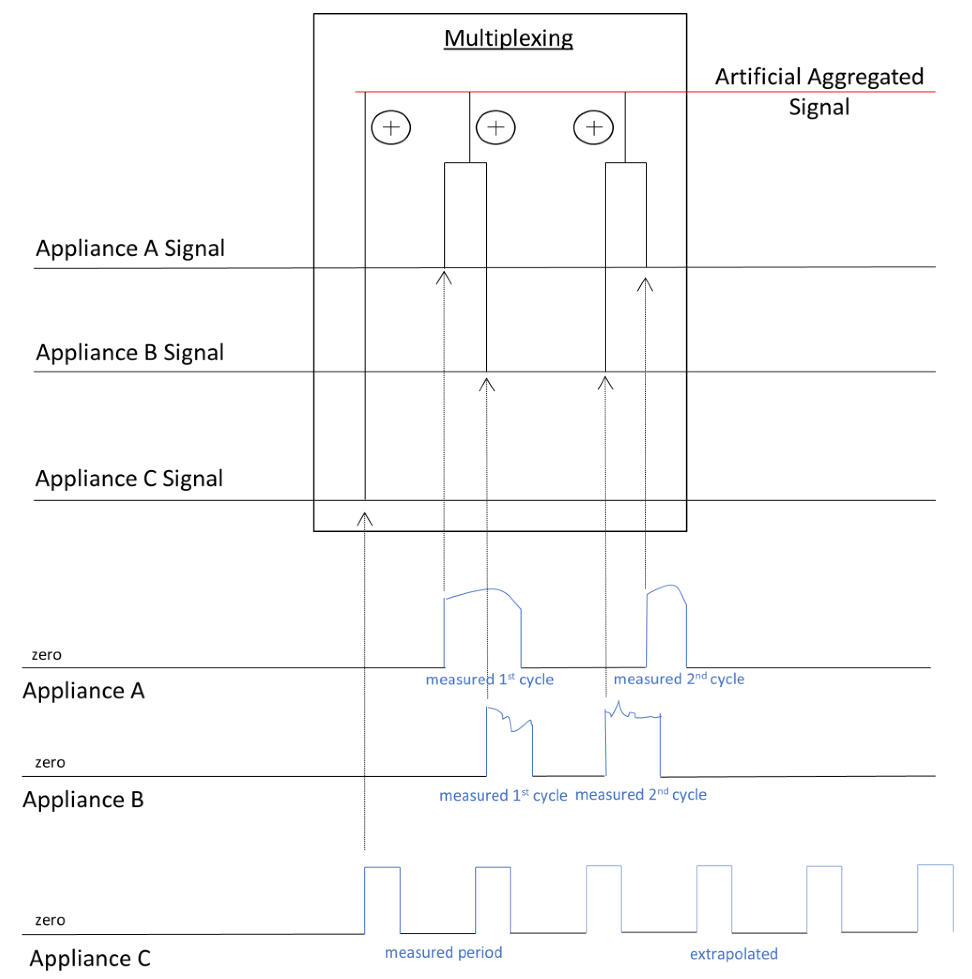
  • Step 2: Most machine learning algorithms require datasets that span ten days for training. To create the artificial total consumption time series, we first extrapolate the series for the appliances of continuous operation to span across the entire sample to create the base load.
  • Step 3: We then combine the signals of the appliances in pairs of two appliances, each time taking one cycle for each appliance, allowing one appliance to start operating and then a couple of seconds/minutes later adding (i.e., “artificially” turning on) the next one. Based on this approach, the algorithm can understand the impact of each appliance and avoid confusing the operation with the other ones.
  • Step 4: We exhaustively repeat the process of the previous step for all pairs of appliances and alternating between the appliances that go first and second.
  • Step 5: Depending on how different the two cycles of each appliance are, the process can be repeated with the second pair of cycles as well.
This process is carried out by the analyst or an entity offering the service (e.g., utility), rather than the consumers themselves, and may also be automated. Additionally, since only cycles of operations are gathered, instead of the operation for a fixed period, the amount of time required can be reduced. We apply an additional constraint that the data gathered in total should not be more than 24 h, representing requirements for the end-user’s engagement for about a single day. The process is schematically presented in Figure 1 in the case of three appliances (“almost” steady, fluctuating, and periodic signal, correspondingly).

2.2. Energy Disaggregation Algorithms

Numerous algorithms have been proposed to perform energy disaggregation, ranging from unsupervised to supervised learning, optimisation models, and event-based algorithms [61]. Although in the inception of the energy disaggregation framework, CO was the method initially proposed by Hart [55], traditionally, it is the FHMM approach that has been widely used in the literature. Recent progress in the machine learning field and especially deep learning, however, has paved the way for the introduction of advanced techniques, such as LSTM, decision trees, and more recently convolution neural networks (CNN) with promising results [62,63] and numerous improvements. The focus of this research is neither to capture the nuances in the latest developments of energy disaggregation algorithms nor to propose a new algorithm altogether. As such, we opt for employing the four most well-established algorithms—CO, FHMMs, decision trees, and LSTM—with a view to testing the protocol and understanding its impact in terms of its performance under restrictive conditions, as well as monitoring their performance in said conditions. In particular, it is expected that data-driven algorithms (such as LSTM networks) perform better in analysing time sequences as they were specially designed for this. The premise of selecting four algorithms that, to some extent, are expected to perform worse—even though this is not given, considering the strict restrictions imposed on data gathering—lies on two reasons. On the one hand, in order to provide a benchmark for the more advanced techniques, and on the other to provide a more holistic evaluation of the efficacy of the protocol under conditions of constraints due to their different theoretical framework. The CO and FHMM algorithms are implemented using the NILMTK toolkit [22], while decision trees and LSTM are developed in python using the Scikit-Learn and Keras Libraries.
The original CO algorithm is based on the premise that, within an installation (e.g., building), both the number of appliances and their state are finite. As such, the problem can be expressed in terms of minimising the difference between the sum of the calculated power consumption of the appliances and the measured aggregated signal. This is described in Equation (2) [55]:
a ^ ( t ) = a rgmin a | P ( t ) n = 1 N a i P i | ,
where a ^ ( t ) is an n-dimension Boolean vector with the predicted state of the n appliances in period t that minimise the error factor in Equation (1), P ( t ) is the real measured aggregated consumption in period t, and P i is the known power consumption of appliance i. More details can be found in [55,64].
HMMs are a probabilistic method widely employed in load monitoring. Their premise lies in estimating the state of N appliances through the means of three variables, expressed as λ = [π, φ, A], where π is a vector representing the initial state of the appliances, A is a matrix representing the possible transitions between states for the appliances, and φ is the emission probability expressing the probability that an appliance receives a certain power consumption value in a specific state and is assumed to follow normal distribution [65]. For a large number of states and appliances, the computational complexity of this process can increase exponentially. As such, FHMMs constitute an expansion of HMMs, introducing multiple independent HMM chains to avoid certain transitions in matrix A and as such, reduce the complexity. The final state of each appliance is then calculated, through a series of algorithms to first estimate the parameters of the HMM (e.g., using forward–backward algorithms), before the most likely sequence of states can be estimated through the Viterbi algorithm [66].
Decision trees are a supervised classification and regression machine learning method with the classification and regression trees (CART) algorithm usually used for NILM problems [67]. They rely on developing a decision tree for each appliance, where the initial aggregated power consumption signal is sequentially split into regions, with the predicted consumption of the appliance taking the average of the appliance observations in the specific region. The method is a top–down approach since the initial node includes the whole dataset and is then split into branches through recursive binary splitting, with each node producing two others (left and right). This split is achieved by defining the cut-point through the minimisation of the residual sum of squares (RSS) (Equation (3)) after considering all possible values [68]:
R S S = j = 1 J i R j ( y i y R j ) ^ 2 ,
where y i refers to the real value and y R j ^ the predicted value in region j. To avoid overfitting and increased training periods, we opt for a max depth value of 8 in the trees developed, since even in cases with more than one predictors the max depth was selected to the value of 10 [69,70,71]. Figure 2 presents the decision tree trained for the air conditioning unit in the case study described below, in Section 2.3.
LSTM-RNN is a widely established option in the literature [72,73,74], constituting an extension of the basic artificial neural networks (ANNs). ANNs constitute graphs that link nodes expressed as neurons, with information passing through the weighted edges from the input to the output layers, passing hidden layers in between (forward pass). Similar to decision trees, the input is the aggregated power consumption, while the output is the power consumption for an appliance (independent models for each appliance). Backpropagation is then used to calibrate the weights between the neurons [75] to minimise a selected error (usually the mean squared error). RNNs expand this process to incorporate past values in the calculations [64], with LSTMs further improving the architecture utilising memory cells addressing RNN memory limitations [33,67]. Here, we employ a simple three-layered network using a 1D layer followed by two bidirectional layers, after standardising the input data, in an approach similar to [33], but instead opting for providing a window of observations as input [76]. The choice of architecture is presented in Table 2.
The 10-day artificial dataset produced based on the previous protocol is split into three subsets for training (four days), internal validation for the model to finetune the hyperparameters (three days), and testing (three days)—which is hidden from the model to perform an out-of-sample test. We note, however, that this out-of-sample test is still performed within the artificial total consumption signal created. To validate the results, we use six widely used metrics—namely, four classification metrics (accuracy, precision, recall, F1 score) that are based on the true/false positive/negative detections and the total positive/negative events [77], and two regression metrics including the mean absolute error (MAE) and the signal aggregate error (SAE) [78].

2.3. Real-Life Application in a Greek Household

The proposed protocol and the algorithms described are tested in a typical Greek household in Athens consisting of two members, which is close to the national average. The data acquisition protocol was applied to collect and multiplex the data from 13 appliances (the core appliances in the household that the experiments took place; in the case of the lights, these are treated as aggregated based on the wiring lines of the household) towards building the artificial database described in the previous section. A Wattson-type meter was used with an amp sensor clip that could collect readings every 30 s (Figure 3). The occupants were advised to perform the measurements according to how they would normally use the appliance (e.g., in the case of the water heater, they were advised not to turn it on and off immediately but rather to use it for heating water as they would do in any typical day). As such, and considering the constraint that data for no more than a day must be collected, the aggregated amount of datapoints gathered across all appliances amounted to 2880. Although this may seem like a small number to produce meaningful results, it is the purpose of this study to test whether even under such constraints, energy disaggregation can produce useful and reliable results.
The signals gathered for the 13 appliances were multiplexed to create the 10-day database that is presented in Figure 4. The final signal for this artificial total consumption constitutes 28,800 datapoints, which are all estimated though the summations of the different appliances, based on the protocol described in the previous section. The signal of the appliances constitutes repetitions of the gathered data based on the two operating cycles collected (or extrapolated in the case of the fridge; again, based on the protocol described in the previous section), while no additional method was employed to expand these signals. As previously discussed, accuracy in the out-of-sample test does not ensure that the protocol is efficient, since this test is still performed within the artificial 10-day database created. As such, we perform one additional test, in which we use the trained models to estimate the load of each appliance based on the real data and measurements of the household’s actual total consumption. In this case, cross-validating the results and using error metrics is not possible since, due to the constraint of using one smart meter, the true consumption of the appliances is not known. Instead, we asked the occupants of the household to keep track of their activities (e.g., time of using an appliance) to perform this check manually. We gathered the data of the total consumption for two full days, along with the timestamps indicated by the occupants, showcasing the exact time they used each appliance (Figure 5 provides an example of these timestamps for one of the two days).

3. Results

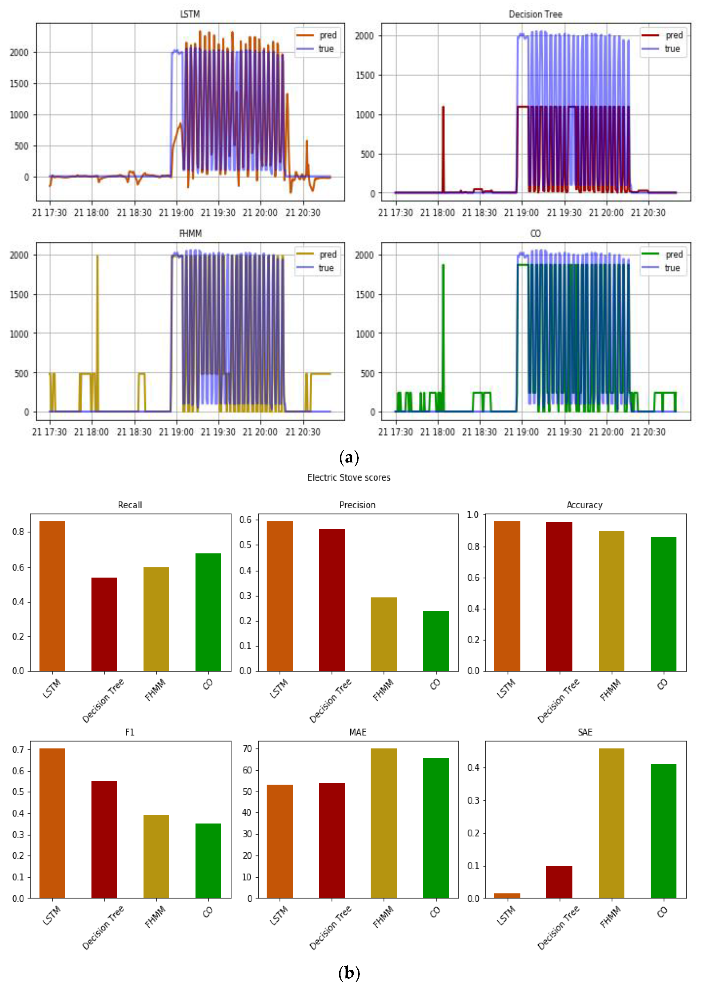
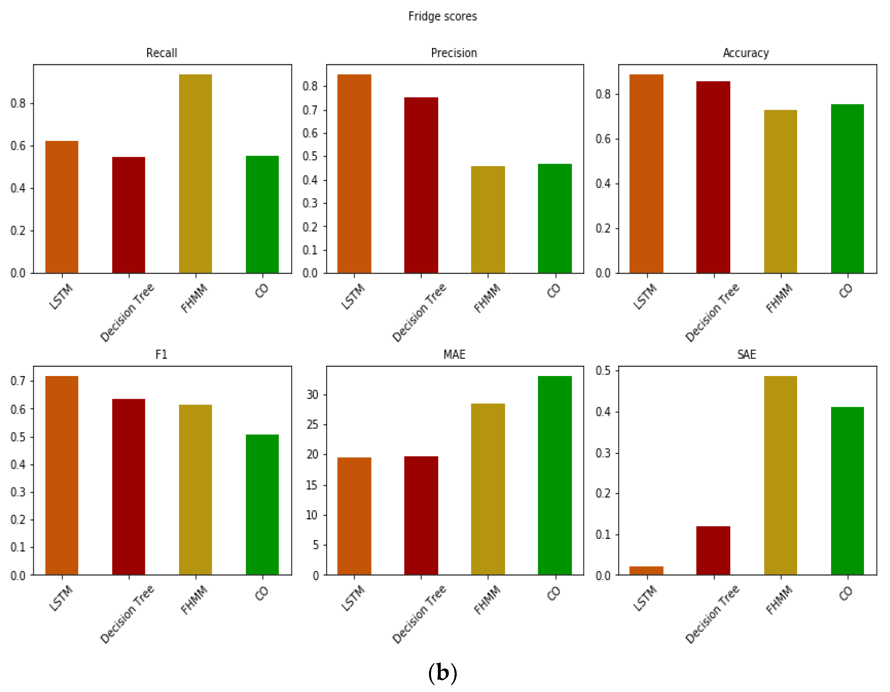
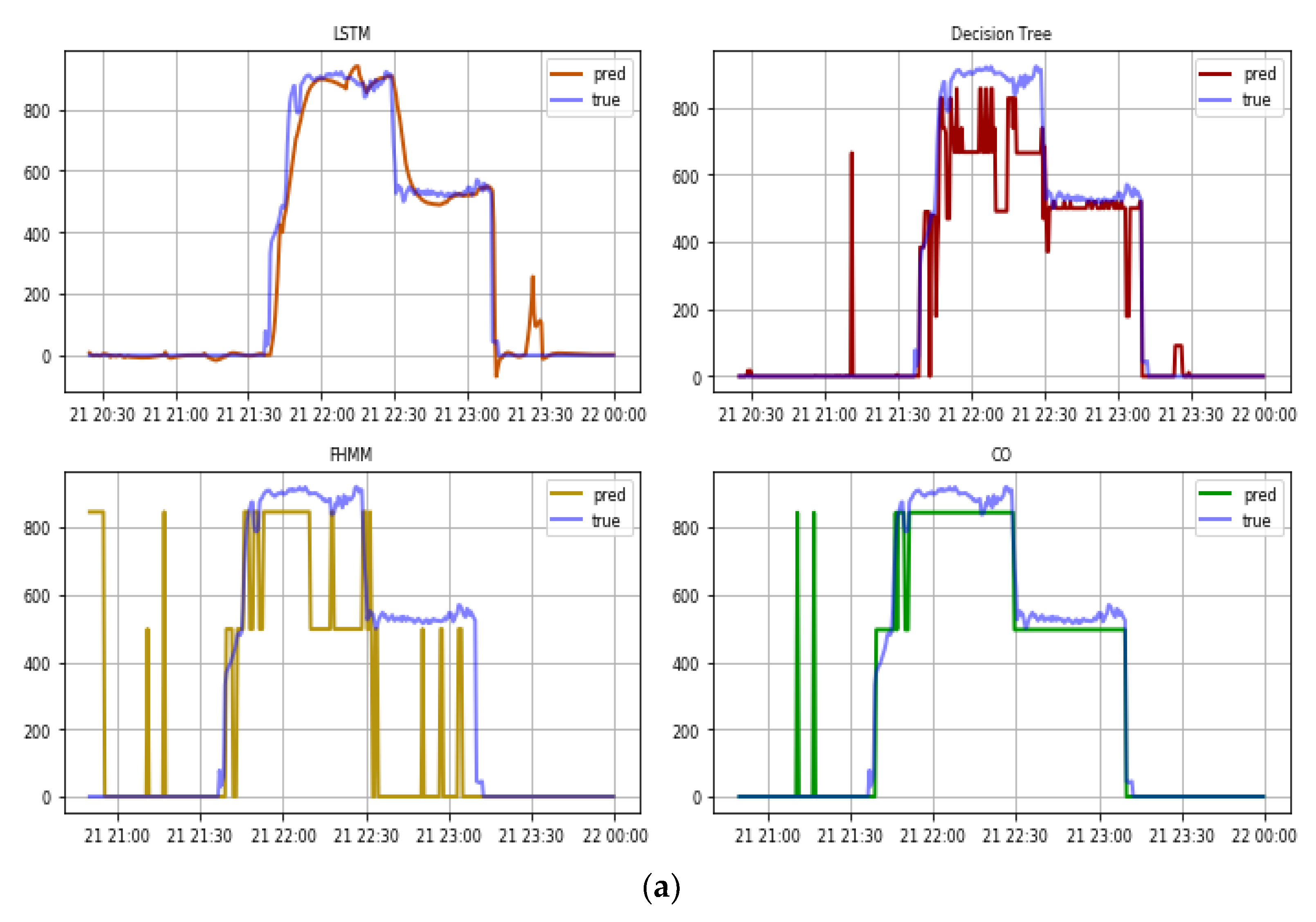
3.1. Out-of-Sample Test

After training and validating the energy disaggregation algorithms, we performed an out-of-sample-test within the artificial database to ensure that the models can accurately understand the patterns of each appliance and easily distinguish them from one another. Based on communications with the occupants, we focused on the five most energy-intensive and highly used appliances, namely, the electric water heater, the electric stove, the fridge, the TV, and the air conditioning unit. These represented roughly 80% of total energy consumption of the household, making them ideal for testing the abilities of the protocol, since lower power appliances are much harder to disaggregate [79]. The computational limitations of CO and FHMMs usually force this constraint to the most energy-intensive appliances, while the two machine learning algorithms do not have this limitation. However, for consistency and an accurate comparison, we analysed the same appliances for all algorithms, with the rest of the 13 appliances still contributing to the training phase.
The water heater (Figure 6) is the largest load of the apartment and operates close to a nominal power of 4 kW with small deviations. These patterns make the water heater a device that can be easily detected, on which NILM typically displays very good performance [80], as reflected in both our time series (Figure 6a) and errors (Figure 6b). In particular, all algorithms managed to correctly identify the time that the water heater was turned on, while throughout the database they do not feature false positive activations, as evident by precision values (close to 1). The estimation of the exact power consumption level was also performed accurately, albeit there are larger differences between the algorithms. The decision tree managed to estimate the operation of the appliance almost perfectly, with the LSTM following closely, with both algorithms benefiting from their ability to provide smoother time series, as reflected in their very good SAE performance. Tracing back to their methodological premise, for an appliance operating steadily through its cycle, it is much easier for the decision trees to identify the correct branch to follow. Consequently, since the values do not fluctuate significantly, estimating the value using the average within the sample of the related branch can yield very accurate results. Contrary to this, the CO and FHMM suggested that the operation of the appliance was at lower power consumption levels for some time during the operation cycle. This stems from the algorithms’ requirement to essentially allocate the total power consumption leading to the necessity of assuming that some other appliances may instead be responsible for part of this signal. In the case of the CO, this is reflected in the low recall, which is triggered by the algorithm’s suggestion that the appliance operates below a 25% threshold of the nominal power, while the FHMM suggests that the appliance operates at 3 kW for a significant amount of time, increasing the MAE. Considering, however, the high power of the appliance, the MAE in all cases is relatively small, leading to all algorithms capturing this appliance relatively accurately.
In contrast, the power of the electric stove (Figure 7) depends largely on its use. We observe that during the heating phase of the oven, power consumption is about 2000 W, while when the temperature reaches the desired value the oven “shuts down”, and the power it absorbs decreases sharply to 100 W, leading to a lot of fluctuations in the signal, expectedly confusing NILM approaches [81]. First, all algorithms managed to accurately estimate the time the appliance turned on and off (from and to zero, respectively)—ignoring the intermediate shifts from high to lower power operation and vice versa—as reflected by the high accuracy value, which was above 0.85 in all cases. Although this is a positive sign, it fails to provide the entire picture, with the estimation for the electric stove (Figure 7a) even intuitively seeming much harder than, e.g., for the water heater. This is a testament that the accuracy metric alone can be misleading, as it only accounts for the true positives/negatives. As a result, in the other metrics that consider false positives/negatives, the scores reflect the difficulties in capturing real behaviour (Figure 7b). Even in this case, though, and despite not fully following the smooth fluctuation of the actual signal during the operation of the oven, LSTM succeeded in predicting the power level of the oven (100–2000 W), while making few incorrect estimates of the intermediate on and off states. As such, the algorithm displayed quite a good performance across all metrics, despite said difficulties. On the contrary, following the fluctuations only slightly worse than LSTM, the decision trees instead suffer from limited capacity to accurately identify the correct power consumption level (0–1200 W instead of the correct 100–2000 W). We observe that the algorithm attempts to establish a mid-value to represent these fluctuations, and in combination with some false negatives, leads to the decision trees suffering in the recall metric, even if the algorithm consistently comes second in all other metrics. The FHMM and CO algorithms further suffer from difficulties in estimating the correct power consumption level, indicating their operation within the 200–500 W range for small periods, leading to very low scores in SAE and F1. Still, the MAE for the stove showed sufficient accuracy, considering that the appliance is considered of high power, like the water heater. Still, this was the highest across all the appliances and for all algorithms, ranging from 50–75 W even though the nominal power of the stove is half that of the water heater (with a MAE of 3–25).
The refrigerator (Figure 8) is a unique appliance in the sense that it is always “on” during the 24 h period. However, due to the existence of a thermostat, it presents a periodic pattern (Figure 8a), with the appliance turning on for a few minutes and then turning off, following this pattern several times during the day (this pattern made it easier to extrapolate the signal to create the artificial database). Due to this easily identifiable pattern, all algorithms managed to follow the correct signal (Figure 8b). However, a common feature found in the estimations is the ability to correctly distinguish the activations of the refrigerator during the early hours of the day, while there is difficulty as the afternoon is approached. This is mainly due to the low operating power of the device, which does not exceed 130 W. Therefore, in the afternoon, when other appliances are also switched on, small fluctuations in the total power due to changes in the condition of the refrigerator can be mistaken for the operation of other loads. On the other hand, in the morning, when not as many devices operate at the same time, we observed a better estimation of the device’s activation and deactivation times. This is reflected in the SAE values of the appliance being the highest among all other appliances and for all algorithms. The issue is most notable in the case of the CO algorithm that consistently performed poorer compared to the other algorithms across most metrics. The same issue is also observed to a lesser extent in the case of the FHMM, and even lower in the case of the decision trees. It is finally negligible in the case of LSTM, although even that experienced fluctuations. Again, LSTM consistently outperformed the other algorithms in most metrics. A notable exception can be found in the FHMM’s high recall value. This evidently hints that the algorithm had a small share of false negatives, indicating that the FHMM did not assume that the refrigerator was off when it was actually operating. This is, however, counterbalanced by a high number of false positives (operations when the appliance is off), reducing precision, and overall leading to an F1 score that is lower than that of decision trees, and the highest MAE and SAE values. Notably, and similar to the stove case, the decision trees also failed to accurately estimate the maximum power consumption level.
The TV (Figure 9) has a low power load (not exceeding 100 W), with increased fluctuations during its operation (Figure 9a), while it is usually switched on mainly in the afternoon and evening hours when various other loads coexist. Therefore, small fluctuations in the overall signal are difficult to accurately be attributed to the operation of the TV. For this reason, and due to their methodological process, CO and FHMM mostly use the TV to represent the total aggregated signal, but without this having any meaningful value. Even in periods when the appliance is on, and the algorithm also indicates that the appliance is on, this cannot be attributed to an accurate estimation, as the algorithm suggests that the appliance is interchanging between on and off for almost the entire duration of the sample period. Consequently, this leads to a poor performance in the metrics (Figure 9b), in particular the regression metrics. The scores can even be considered overoptimistic of the performance of the algorithms, since the randomly accurate estimations may yield a better picture than actually exists. This is especially the case for the recall metric that does not consider false positives—contrary to precision which does and penalises these two approaches. The same can be said for decision trees, but in this case, the estimation of the algorithm does not seem entirely random. In the instances when the appliance was actually on, there was an increase in the average estimation of the power consumption throughout the period of operation, with the estimated power consumption even rarely reaching zero in said period, contrary to when the appliance was actually off. As such, the performance of the decision trees in the error metrics is consistently higher than the other two algorithms. Similarly, the performance of the decision trees in estimating the operation of the TV was not fundamentally different than that of the stove, an appliance that was easier to identify when it is turned on but difficult to estimate the true power consumption level and follow the fluctuations. Even better than decision trees, we get stronger indication that the LSTM algorithm actually follows the patterns of the appliance, with the algorithm easily performing better than the other three. As shown in the upper left panel of Figure 9a, the predicted signal is not just white noise but, apart from one instance, the algorithm actually manages to accurately follow the real consumption. On the other hand, there is an underestimation of the power level of the device during its operating periods leading to a non-negligible MAE relative to the very small nominal power of the appliance, but which is still not very large compared to both the other appliances and the negligible SAE. This indicates that, even in the challenging task of estimating the operation of appliances with lower power consumption levels [82], the LSTM-based NILM may perform well.
Finally, the air conditioning unit (Figure 10) is an appliance with an interesting pattern lying in between the water heater and the stove, in the sense that its power consumption fluctuated between 400 and 1000 W in steps—like the stove—depending on both its use and the external environmental conditions. However, within these two levels of operation, the power consumption was almost steady for significant amounts of time—like the water heater (Figure 10a). We note that the use of the AC referred to the heating mode, as measurements were gathered during winter months. Unlike the stove, and similar to the water heater, all algorithms had a fairly good accuracy in their estimations (Figure 9b), indicating that long periods of steady signal make it easier for NILM to provide a better estimate, even if there are some fluctuations within the same appliance. Again, the LSTM algorithm had an overall very good performance as reflected in all metrics, with negligible MAE and SAE, indicating a high accuracy in terms of estimating the consumption of the appliance, despite said appliance also being of high power. Interestingly, the CO algorithm, which failed to stand out among the other appliances, in this case managed to monitor the operation of the appliance very closely, as is reflected in the very high value of recall (visually highlighted in the lower right panel of Figure 10a). However, despite the algorithm operating excellently when the appliance was on, it was also associated with many false positives. These, although not traceable in the subset of the database presented in Figure 10a, existed in the rest of the data, as is reflected in the poor scores of precision (much lower in high contrast with the recall) and SAE. The decision trees also performed well, featuring the common issue identified in the previous appliances of estimating the operation but underestimating the power consumption level—in this case only in the highest consumption state. In contrast, the FHMM algorithm faced considerable challenges overall, finding it hard to follow the consumption levels, especially the lower state, while suffering from a high share of false positives in the whole database. We should note, however, that since only two cycles were measured for the appliance, there was not a high level of differentiation in the use of the appliance, which is expected for AC units. As such, the following test of the true total consumption data is necessary to strengthen our results here.

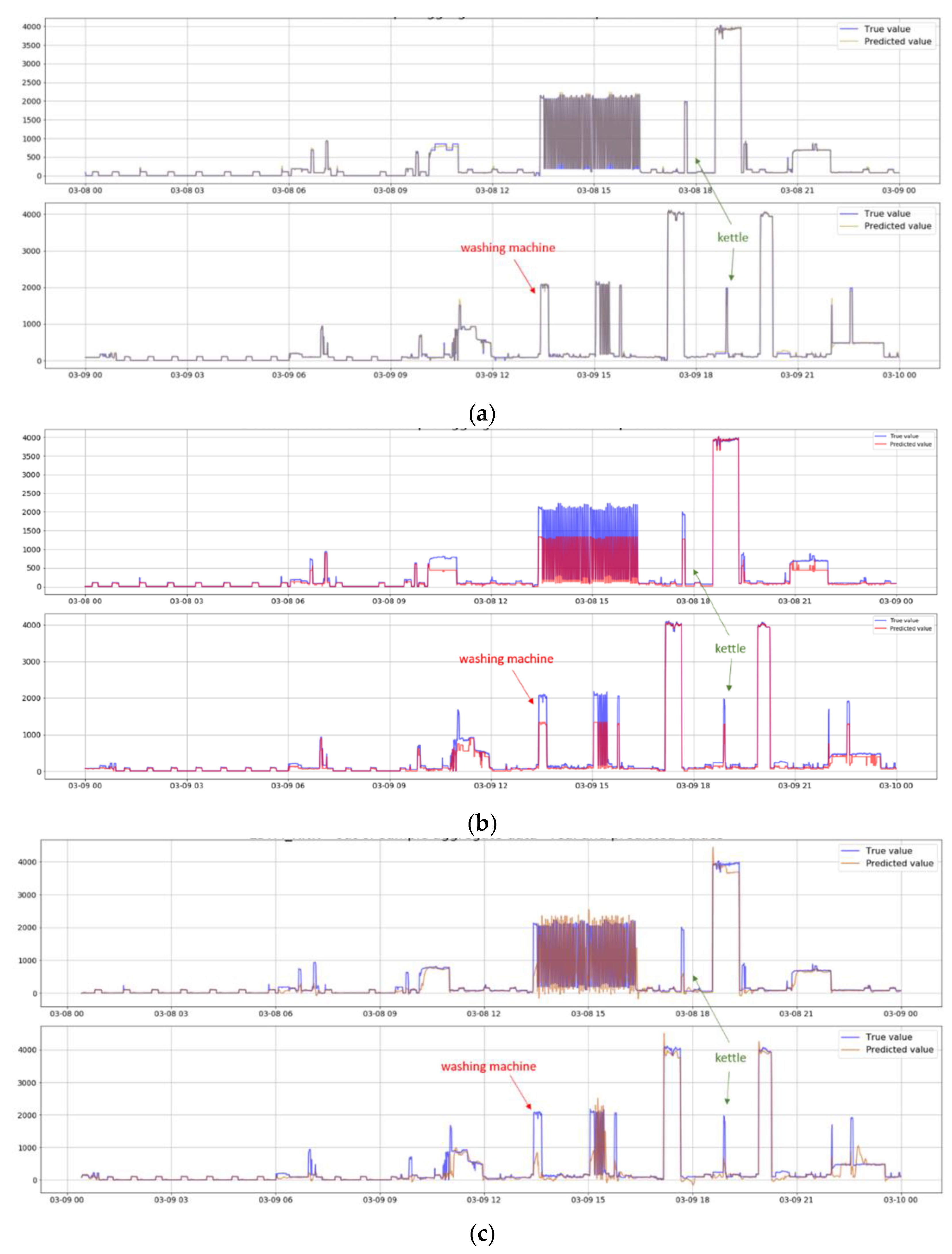
3.2. External Test in Real Total Consumption Data

In this final test, we aimed to capture the protocol’s ability to provide accurate estimations for the operating load of each appliance, based on real data on the household’s total consumption. In particular, the previous test was able to confirm that the trained models were sufficiently able to identify the patterns of the appliances, with some performing better than others (e.g., LSTM and decision trees) or for some appliances (e.g., water heater). However, since it was performed within the artificial database, that test provided little information on the ability of the algorithms to identify the appliances’ operation and fluctuations in real-life conditions. Performing such a test in a real-life total consumption signal has the challenge of no real data existing for the appliances that could be used to cross-validate the estimations, as already discussed in Section 2.3. However, summing the estimated signal of the appliances and comparing with the total signal can provide a first estimation of the performance of the algorithms. In the case of the FHMM and CO, their methodological premise forces the algorithms to always match the total signal with the appliances selected to be analysed (in our case the five appliances discussed in Section 3.1). On the contrary, the LSTM and decision trees offer some flexibility on this front. These results are presented in Figure 11, where CO is omitted since it shares the same performance to that of FHMM.
With the assistance of the occupants, we have timestamped two other notable appliances: the washing machine and the kettle. In the case of the FHMM and CO, due to the restriction that the algorithms had to match the total consumption, the respective signals indicating the operation of these two appliances were mis-labelled as the operation of one of the five appliances analysed. This restriction does not apply in the case of the decision trees and LTSM and consequently such issues appear to a lesser extent. Hence, the concentration of the false positive estimations from the CO and FHMM was much higher than the other two algorithms, validating concerns triggered in the tests performed in Section 3.1. On the contrary, the SAE of LSTM and the decision trees—which is only meaningful to calculate for these two algorithms—was measured at 0.0982 and 0.235, respectively. The losses appeared as a result of the appliances omitted and some performance difficulties, especially in the case of the decision trees (e.g., stove). This further validates their good performance, while their ability to analyse more appliances, which we opted not to do in this research for comparative reasons, provides encouraging signs for further improvement.
Delving into the results of these two algorithms on the appliance level (Figure 12), and focusing first on the high-power appliances, it is evident that the models could easily identify the operation of the water heater, including a correct estimation of the level of power. The same can be said about the two phases of operation of the AC unit, for which LSTM was also able to identify the appliance’s operation, including the correct range of power, albeit with a greater error compared to the water heater. This error was more notable in the case of the decision trees, reproducing issues identified in the test within the artificial database. This ability, however, to follow the operation of the device even with the smaller or larger deviations from the correct level is still important, since, contrary to the water heater, the AC unit can experience some fluctuations that are not always the same during the operation phase, and which may not be included in the artificial total signal. The algorithms were actually able to follow the operation of the appliance, even if they were not specifically trained on these exact patterns, which provides evidence that a protocol based on the artificial total signal approach followed can provide accurate results. On the other hand, and as with the original test, the pattern of the electric stove does not completely capture the smooth fluctuation of the actual signal but still follows the operation to a sufficient extent in the case of LSTM, identifying the operation of the appliance, and closely following the power consumption. Again, in the case of the decision trees, the same issue of failing to capture the exact power consumption level appeared. However, this is still interesting, as it seems that the algorithms repeat the behaviours found in the test in the artificial database, which is not a given as the artificial total consumption signal is markedly different to the real one. Therefore, the ability or inability to follow the operation of the appliance is as a result of the algorithm, and the constrained data acquisition protocol does not introduce notable sources of error, thereby attesting to its potential use in NILM approaches. In these three appliances, false positive triggers are limited, with such instances distinguishable and of small width—i.e., that they can be considered negligible.
The two algorithms, finally, show difficulty in identifying the operation of the appliances with low power, such as refrigerators and televisions, during periods of operation under heavy loads. This was particularly evident when the electric stove was operating, since due to its fluctuation, the algorithms showed signs of conflict, thinking that some parts of this fluctuation should be attributed to the small appliances (in this case the fridge and the TV). However, when accurately identifying the operation, the signal for the two devices was as smooth as the real data, again showing similar behaviour to the original test, thus realistically reflecting their actual operating pattern. For example, this is evident in the identification of the fridge during the morning when the other appliances were switched off. For the TV, we can see that the LSTM algorithm accurately identified the correct periods that the TV was indeed on, but in both appliances there were expediently more incorrect activations. Yet, there are some positive signs, since in the first two activations of the TV, even though it was very early in the morning (in particular, at 6 AM), the algorithm indicated that the TV was on. When we cross-validated this output with the occupants, they confirmed that turning the TV on at that time was part of their morning routine. Evidently, this example is encouraging in terms of the protocol’s ability to identify behavioural energy patterns, even under constraints in the use of smart infrastructure and for a low-consumption appliance.

4. Conclusions

Energy disaggregation algorithms could be the turning point for reducing the amount of equipment required to provide tailor-made insights to end-users regarding their energy consumption and help them towards becoming more energy conscious. This would consequently lead to reduced energy costs, as well as contribute, from a broader energy policy perspective, to achieving the ambitious energy and emissions reductions targets in the building sector. Significant limitations, however, remain regarding the use of public datasets or measuring data on the ground. In this research, we presented a protocol for data acquisition based on real-life measurements in the same household that the solution was intended to be applied to, constraining the number of smart meters to just one and the data gathering process to less than a day to avoid the occupants losing interest. Using four well-established and widely used algorithms in the NILM field and in a case study of a typical Greek household, we first sought to understand if energy disaggregation through the presented protocol under constraints can provide meaningful results. Second, we aimed to capture how the different algorithms perform and whether energy disaggregation’s ability to provide tips for behaviour-induced energy savings is maintained under constraints.
In particular, we introduced a protocol for appropriately multiplexing the signal from the independent measurements of appliances to create an artificial total consumption signal and train the algorithms based on it. This was instead of measuring a real total consumption that would require at least one additional smart meter. We found such a protocol promising, as it showcased the accurate identification of the operation of the key household appliances, especially with the use of machine learning and deep learning decision trees and LSTM algorithms and the energy-intensive appliances: the electric water heater, the air conditioning unit, and to some extent—albeit with some difficulties due to extensive fluctuations—the electric stove. This approach was also found promising regarding the identification of the operation of the low-power appliances, albeit to a smaller extent than the high-power devices. Notably, we managed to accurately represent the behavioural patterns of the occupants, and therefore confirm that energy disaggregation can provide meaningful tips for energy efficiency even under constraints using the introduced protocol. In addition, we found that using an artificial signal for the training phase, and then applying the models to the real total signal, did not induce additional errors other than those inherently part of the models themselves. The four employed models showcased similar trends in both the artificial and the real signal tests, providing further evidence on the appropriateness of the protocol and energy disaggregation itself even under constraints.
From the algorithms’ perspective, despite the overall positive signs, some algorithms performed better than others. In particular, both of the more advanced machine and deep learning techniques, namely, the decision trees and LSTM, consistently outperformed the more traditionally used CO and FHMM across all tests, most metrics, and appliances. The LSTM algorithm showed the most promising signs, consistently capturing the activation events as well as the operation level of the appliances (even in many cases the lower-consumption ones), introducing small amounts of false positive and negative indications. The decision trees closely followed the performance of LSTM and, despite some difficulties regarding the accurate estimation of the power consumption level, presented some advantages in the case of the water heater, which is a cornerstone electricity consumption appliance of a household. Moreover, the significantly lower amount required to train them may prove an added advantage to counterbalance the smaller accuracy (compared to LSTM). On the other hand, the CO and FHMM faced more difficulties as a result of their methodological approach to allocating appliances to the total signal with their performance being associated with numerous false positive/negative indications. Still, these algorithms had some niche advantages, with the CO algorithm following very closely the time series of the AC unit, albeit with a lot of false positives when the appliance was off, while this was also the case for FHMM algorithm in the case of the fridge. This indicates that hybrid approaches that exploit the advantages of different methods, much like in NILM [83,84], may be promising under constraints and restrictions such as those imposed in this study.
For the field of energy disaggregation in general, the results of this study offer insights into the requirements and directions for future research. Although the use of public datasets representing specific households is an important route of research, gathering real-life data from the households themselves is also important. The fact that our study proved efficient without measuring the true consumption but instead getting measurements only from the appliances, indicates that it is the appliances that mostly drive these patterns. As such, focusing on the signals of the appliances and building datasets at that level (e.g., COOLL, WHITED, and PLAID—see Table 1), instead of silo households (e.g., on public datasets), could also be a promising route. But such an approach would also require much effort, since appliances of different nominal characteristics may behave differently and it is important for these databases to incorporate a wide variety of different types of appliances.
Excluding the restriction imposed by the research design itself, namely the constraints on the equipment and duration of measurement, additional caveats include the restriction of the LSTM and decision tree models to analyse only five appliances for consistency with the CO and FHMM algorithms. Future research can increase the number of appliances analysed, use more recent methods (including CNNs), or even simply further calibrate the parameters of the algorithms employed here, like the max depth of the decision trees. Additionally, our study sought to understand whether specific constraints still allow for the effective use of energy disaggregation. On top of our positive results for most appliances and the specific limitations reached in the case of some low-consumption appliances, further studies can delve into the minimum number of conditions to still provide valuable results, inter alia establishing processes to automate the signal multiplexing introduced by our protocol. Since our study presented difficulties for the protocol to always identify the appliances of low power, further research can shed light on these aspects and suggest ways to improve the protocol’s ability to better capture these appliances as well. Finally, since our protocol is based on data gathered in the same household as the real case test is performed, it is bound to perform better than using models trained in existing databases, including appliances that may not match the ones in the test household (regarding the level of power consumption and/or overall behaviour of the appliance). However, further experiments in real households that compare these two approaches, i.e., the protocol employed here, and training models based on some of the databases presented in Table 1, could further validate and quantify the added value of the protocol.

Author Contributions

Conceptualization, K.K. and A.N.; methodology, K.K. and V.M.; software, K.K. and N.D.; validation, K.K., A.N. and H.D.; formal analysis, K.K. and N.D.; investigation, K.K. and A.N.; resources, V.M.; data curation, K.K. and N.D.; writing—original draft preparation, K.K. and A.N.; writing—review and editing, K.K., V.M., H.D., N.D., A.K. and A.N.; visualization, K.K. and N.D.; supervision, V.M., H.D. and A.N.; project administration, V.M.; funding acquisition, V.M. and H.D. All authors have read and agreed to the published version of the manuscript.

Funding

This research was funded by the European Commission Horizon 2020 Framework Programme, ‘BD4NRG’ Research and Innovation Project, grant number 872613, and by the Hellenic Foundation for Research and Innovation (HFRI) and the General Secretariat for Research and Innovation (GSRI) project “ATOM—Innovative Personalised Apps to Motivate and Support Behavioural Energy Efficiency”, grant agreement no. HFRI-FM17-2566. The APC was funded by the National Technical University of Athens.

Data Availability Statement

The data presented in this study are openly available in Zenodo at 10.5281/zenodo.10046682, reference number [reference number].

Acknowledgments

The most important part of this research is based on the H2020 European Commission Project “BD4NRG” under grant agreement No. 872613 and the Hellenic Foundation for Research and Innovation (HFRI) and the General Secretariat for Research and Innovation (GSRI) project “ATOM” under grant agreement no. HFRI-FM17-2566. The sole responsibility for the content of this paper lies with the authors. The paper does not necessarily reflect the opinions of the European Commission and the Greek government.

Conflicts of Interest

The authors declare no conflict of interest. The funders had no role in the design of the study; in the collection, analyses, or interpretation of the data; in the writing of the manuscript, or in the decision to publish the results.

References

  1. Domorenok, E.; Graziano, P. Understanding the European Green Deal: A Narrative Policy Framework Approach. Eur. Policy Anal. 2023, 9, 9–29. [Google Scholar] [CrossRef]
  2. Fouquet, D.; Traum, Y. Steps Forward in the Implementation of the Green Deal. Renew. Energy Law Policy Rev. 2023, 11, 33–34. [Google Scholar] [CrossRef]
  3. Buckley, N.; Mills, G.; Reinhart, C.; Berzolla, Z.M. Using Urban Building Energy Modelling (UBEM) to Support the New European Union’s Green Deal: Case Study of Dublin Ireland. Energy Build. 2021, 247, 111115. [Google Scholar] [CrossRef]
  4. Kougias, I.; Taylor, N.; Kakoulaki, G.; Jäger-Waldau, A. The Role of Photovoltaics for the European Green Deal and the Recovery Plan. Renew. Sustain. Energy Rev. 2021, 144, 111017. [Google Scholar] [CrossRef]
  5. Koasidis, K.; Marinakis, V.; Nikas, A.; Chira, K.; Flamos, A.; Doukas, H. Monetising Behavioural Change as a Policy Measure to Support Energy Management in the Residential Sector: A Case Study in Greece. Energy Policy 2022, 161, 112759. [Google Scholar] [CrossRef]
  6. Boemi, S.-N.; Papadopoulos, A.M. Energy Poverty and Energy Efficiency Improvements: A Longitudinal Approach of the Hellenic Households. Energy Build. 2019, 197, 242–250. [Google Scholar] [CrossRef]
  7. Kanellou, E.; Hinsch, A.; Vorkapić, V.; Torres, A.-D.; Konstantopoulos, G.; Matsagkos, N.; Doukas, H. Lessons Learnt and Policy Implications from Implementing the POWERPOOR Approach to Alleviate Energy Poverty. Sustainability 2023, 15, 8854. [Google Scholar] [CrossRef]
  8. Marinakis, V. Big Data for Energy Management and Energy-Efficient Buildings. Energies 2020, 13, 1555. [Google Scholar] [CrossRef]
  9. Pisello, A.L.; Castaldo, V.L.; Piselli, C.; Fabiani, C.; Cotana, F. How Peers’ Personal Attitudes Affect Indoor Microclimate and Energy Need in an Institutional Building: Results from a Continuous Monitoring Campaign in Summer and Winter Conditions. Energy Build. 2016, 126, 485–497. [Google Scholar] [CrossRef]
  10. Lopes, M.; Antunes, C.H.; Janda, K.B. Energy and Behaviour: Towards a Low Carbon Future; Academic Press: Cambridge, MA, USA, 2019; ISBN 978-0-12-818568-1. [Google Scholar]
  11. Mundaca, L.; Zhu, X.; Hackenfort, M. Behavioural Insights for Sustainable Energy Use. Energy Policy 2022, 171, 113292. [Google Scholar] [CrossRef]
  12. Grubler, A.; Wilson, C.; Bento, N.; Boza-Kiss, B.; Krey, V.; McCollum, D.L.; Rao, N.D.; Riahi, K.; Rogelj, J.; De Stercke, S.; et al. A Low Energy Demand Scenario for Meeting the 1.5 °C Target and Sustainable Development Goals without Negative Emission Technologies. Nat. Energy 2018, 3, 515–527. [Google Scholar] [CrossRef]
  13. Azevedo, I.; Bataille, C.; Bistline, J.; Clarke, L.; Davis, S. Net-Zero Emissions Energy Systems: What We Know and Do Not Know. Energy Clim. Chang. 2021, 2, 100049. [Google Scholar] [CrossRef]
  14. International Energy Agency Net Zero by 2050: A Roadmap for the Global Energy Sector 2021. Available online: https://www.iea.org/reports/net-zero-by-2050 (accessed on 1 September 2023).
  15. Lopes, M.A.R.; Antunes, C.H.; Martins, N. Towards More Effective Behavioural Energy Policy: An Integrative Modelling Approach to Residential Energy Consumption in Europe. Energy Res. Soc. Sci. 2015, 7, 84–98. [Google Scholar] [CrossRef]
  16. Hu, S.; Yan, D.; Azar, E.; Guo, F. A Systematic Review of Occupant Behavior in Building Energy Policy. Build. Environ. 2020, 175, 106807. [Google Scholar] [CrossRef]
  17. Perlaviciute, G. Contested Climate Policies and the Four Ds of Public Participation: From Normative Standards to What People Want. WIREs Clim. Chang. 2022, 13, e749. [Google Scholar] [CrossRef]
  18. Van den Broek, K.L. Household Energy Literacy: A Critical Review and a Conceptual Typology. Energy Res. Soc. Sci. 2019, 57, 101256. [Google Scholar] [CrossRef]
  19. Gerasopoulos, S.I.; Manousakis, N.M.; Psomopoulos, C.S. Smart Metering in EU and the Energy Theft Problem. Energy Effic. 2022, 15, 12. [Google Scholar] [CrossRef]
  20. Shin, C.; Rho, S.; Lee, H.; Rhee, W. Data Requirements for Applying Machine Learning to Energy Disaggregation. Energies 2019, 12, 1696. [Google Scholar] [CrossRef]
  21. Verma, A.; Anwar, A.; Mahmud, M.A.P.; Ahmed, M.; Kouzani, A. A Comprehensive Review on the NILM Algorithms for Energy Disaggregation. arXiv 2021, arXiv:2102.12578. [Google Scholar]
  22. Batra, N.; Kukunuri, R.; Pandey, A.; Malakar, R.; Kumar, R.; Krystalakos, O.; Zhong, M.; Meira, P.; Parson, O. Towards Reproducible State-of-the-Art Energy Disaggregation. In Proceedings of the 6th ACM International Conference on Systems for Energy-Efficient Buildings, Cities, and Transportation, New York, NY, USA, 13–14 November 2019; Association for Computing Machinery: New York, NY, USA, 2019; pp. 193–202. [Google Scholar]
  23. Barker, S.; Mishra, A.; Irwin, D.; Cecchet, E.; Shenoy, P.; Albrecht, J. Smart*: An Open Data Set and Tools for Enabling Research in Sustainable Homes. In Proceedings of the 2012 Workshop on Data Mining Applications in Sustainability, Beijing, China, 12 August 2012. [Google Scholar]
  24. Kolter, J.Z.; Johnson, M.J. REDD: A Public Data Set for Energy Disaggregation Research. Artif. Intell. 2011, 25, 59–62. [Google Scholar]
  25. Dash, S.; Sahoo, N.C. Electric Energy Disaggregation via Non-Intrusive Load Monitoring: A State-of-the-Art Systematic Review. Electr. Power Syst. Res. 2022, 213, 108673. [Google Scholar] [CrossRef]
  26. Pereira, L.; Nunes, N. Performance Evaluation in Non-Intrusive Load Monitoring: Datasets, Metrics, and Tools—A Review. WIREs Data Min. Knowl. Discov. 2018, 8, e1265. [Google Scholar] [CrossRef]
  27. Anderson, K.D.; Ocneanu, A.; Carlson, D.R.; Rowe, A.G.; Berges, M. BLUED: A Fully Labeled Public Dataset for Event-Based Non-Intrusive Load Monitoring Research. In Proceedings of the 2nd KDD Workshop on Data Mining Applications in Sustainability, Beijing, China, 12–16 August 2012. [Google Scholar]
  28. Jazizadeh, F.; Afzalan, M.; Becerik-Gerber, B.; Soibelman, L. EMBED: A Dataset for Energy Monitoring through Building Electricity Disaggregation. In Proceedings of the Ninth International Conference on Future Energy Systems, Karlsruhe, Germany, 12–15 June 2018; Association for Computing Machinery: New York, NY, USA, 2018; pp. 230–235. [Google Scholar]
  29. Reinhardt, A.; Baumann, P.; Burgstahler, D.; Hollick, M.; Chonov, H.; Werner, M.; Steinmetz, R. On the Accuracy of Appliance Identification Based on Distributed Load Metering Data. In Proceedings of the 2012 Sustainable Internet and ICT for Sustainability (SustainIT), Pisa, Italy, 4–5 October 2012; pp. 1–9. [Google Scholar]
  30. Makonin, S.; Popowich, F.; Bartram, L.; Gill, B.; Bajić, I.V. AMPds: A Public Dataset for Load Disaggregation and Eco-Feedback Research. In Proceedings of the 2013 IEEE Electrical Power & Energy Conference, Halifax, NS, Canada, 21–23 August 2013; pp. 1–6. [Google Scholar]
  31. Batra, N.; Gulati, M.; Singh, A.; Srivastava, M.B. It’s Different: Insights into Home Energy Consumption in India. In Proceedings of the 5th ACM Workshop on Embedded Systems For Energy-Efficient Buildings, Roma, Italy, 13–14 November 2013; Association for Computing Machinery: New York, NY, USA, 2013; pp. 1–8. [Google Scholar]
  32. Beckel, C.; Kleiminger, W.; Cicchetti, R.; Staake, T.; Santini, S. The ECO Data Set and the Performance of Non-Intrusive Load Monitoring Algorithms. In Proceedings of the 1st ACM Conference on Embedded Systems for Energy-Efficient Buildings, Memphis, TN, USA, 3–6 November 2014; Association for Computing Machinery: New York, NY, USA, 2014; pp. 80–89. [Google Scholar]
  33. Kelly, J.; Knottenbelt, W. Neural Nilm: Deep Neural Networks Applied to Energy Disaggregation. In Proceedings of the 2nd ACM International Conference on Embedded Systems for Energy-Efficient Built Environments, Seoul, Republic of Korea, 4–5 November 2015. [Google Scholar]
  34. Monacchi, A.; Egarter, D.; Elmenreich, W.; D’Alessandro, S.; Tonello, A.M. GREEND: An Energy Consumption Dataset of Households in Italy and Austria. In Proceedings of the 2014 IEEE International Conference on Smart Grid Communications (SmartGridComm), Venice, Italy, 3–6 November 2014; pp. 511–516. [Google Scholar]
  35. Murray, D.; Liao, J.; Stankovic, L.; Stankovic, V.; Hauxwell-Baldwin, R.; Wilson, C.; Coleman, M.; Kane, T.; Firth, S. A Data Management Platform for Personalised Real-Time Energy Feedback: 8th International Conference on Energy Efficiency in Domestic Appliances and Lighting. In Proceedings of the 8th International Conference on Energy Efficiency in Domestic Appliances and Lighting, Lucerne, Switzerland, 26–28 August 2015. [Google Scholar]
  36. Parson, O.; Fisher, G.; Hersey, A.; Batra, N.; Kelly, J.; Singh, A.; Knottenbelt, W.; Rogers, A. Dataport and NILMTK: A Building Data Set Designed for Non-Intrusive Load Monitoring. In Proceedings of the 2015 IEEE Global Conference on Signal and Information Processing (GlobalSIP), Orlando, FL, USA, 14–16 December 2015; pp. 210–214. [Google Scholar]
  37. Gisler, C.; Ridi, A.; Zufferey, D.; Khaled, O.A.; Hennebert, J. Appliance Consumption Signature Database and Recognition Test Protocols. In Proceedings of the 2013 8th International Workshop on Systems, Signal Processing and their Applications (WoSSPA), Algiers, Algeria, 12–15 May 2013; pp. 336–341. [Google Scholar]
  38. Makonin, S. HUE: The Hourly Usage of Energy Dataset for Buildings in British Columbia. Data Brief 2019, 23, 103744. [Google Scholar] [CrossRef] [PubMed]
  39. Saldanha, N.; Beausoleil-Morrison, I. Measured End-Use Electric Load Profiles for 12 Canadian Houses at High Temporal Resolution. Energy Build. 2012, 49, 519–530. [Google Scholar] [CrossRef]
  40. Makonin, S.; Wang, Z.J.; Tumpach, C. RAE: The Rainforest Automation Energy Dataset for Smart Grid Meter Data Analysis. Data 2018, 3, 8. [Google Scholar] [CrossRef]
  41. Kriechbaumer, T.; Jacobsen, H.-A. BLOND, a Building-Level Office Environment Dataset of Typical Electrical Appliances. Sci. Data 2018, 5, 180048. [Google Scholar] [CrossRef] [PubMed]
  42. Picon, T.; Meziane, M.N.; Ravier, P.; Lamarque, G.; Novello, C.; Bunetel, J.-C.L.; Raingeaud, Y. COOLL: Controlled On/Off Loads Library, a Public Dataset of High-Sampled Electrical Signals for Appliance Identification. arXiv 2016, arXiv:1611.05803. [Google Scholar]
  43. Chen, V.L.; Delmas, M.A.; Locke, S.L.; Singh, A. Dataset on Information Strategies for Energy Conservation: A Field Experiment in India. Data Brief 2018, 16, 713–716. [Google Scholar] [CrossRef]
  44. Uttama Nambi, A.S.N.; Reyes Lua, A.; Prasad, V.R. LocED: Location-Aware Energy Disaggregation Framework. In Proceedings of the 2nd ACM International Conference on Embedded Systems for Energy-Efficient Built Environments, Seoul, Republic of Korea, 4–5 November 2015; Association for Computing Machinery: New York, NY, USA, 2015; pp. 45–54. [Google Scholar]
  45. Gao, J.; Giri, S.; Kara, E.C.; Bergés, M. PLAID: A Public Dataset of High-Resoultion Electrical Appliance Measurements for Load Identification Research: Demo Abstract. In Proceedings of the 1st ACM Conference on Embedded Systems for Energy-Efficient Buildings, Seoul, Republic of Korea, 4–6 November 2014; Association for Computing Machinery: New York, NY, USA, 2014; pp. 198–199. [Google Scholar]
  46. Kahl, M.; Haq, A.; Kriechbaumer, T.; Jacobsen, H. WHITED-A Worldwide Household and Industry Transient Energy Data Set. In Proceedings of the 3rd International Workshop on Non-Intrusive Load Monitoring, Vancouver, BC, Canada, 14–15 May 2016. [Google Scholar]
  47. Shin, C.; Lee, E.; Han, J.; Yim, J.; Rhee, W.; Lee, H. The ENERTALK Dataset, 15 Hz Electricity Consumption Data from 22 Houses in Korea. Sci. Data 2019, 6, 193. [Google Scholar] [CrossRef]
  48. Pereira, L.; Quintal, F.; Gonçalves, R.; Nunes, N.J. SustData: A Public Dataset for ICT4S Electric Energy Research; Atlantis Press: Amsterdam, The Netherlands, 2014; pp. 359–368. [Google Scholar]
  49. Ribeiro, M.; Pereira, L.; Quintal, F.; Nunes, N. SustDataED: A Public Dataset for Electric Energy Disaggregation Research; Atlantis Press: Amsterdam, The Netherlands, 2016; pp. 244–245. [Google Scholar]
  50. Chavan, D.R.; More, D.S.; Khot, A.M. IEDL: Indian Energy Dataset with Low Frequency for NILM. Energy Rep. 2022, 8, 701–709. [Google Scholar] [CrossRef]
  51. Pullinger, M.; Kilgour, J.; Goddard, N.; Berliner, N.; Webb, L.; Dzikovska, M.; Lovell, H.; Mann, J.; Sutton, C.; Webb, J.; et al. The IDEAL Household Energy Dataset, Electricity, Gas, Contextual Sensor Data and Survey Data for 255 UK Homes. Sci. Data 2021, 8, 146. [Google Scholar] [CrossRef] [PubMed]
  52. Yan, L.; Han, J.; Xu, R.; Li, Z. LIFTED: Household Appliance-Level Load Dataset and Data Compression with Lossless Coding Considering Precision. In Proceedings of the 2020 IEEE Power & Energy Society General Meeting (PESGM), Montreal, QC, Canada, 2–6 August 2020; pp. 1–5. [Google Scholar]
  53. Pipattanasomporn, M.; Chitalia, G.; Songsiri, J.; Aswakul, C.; Pora, W.; Suwankawin, S.; Audomvongseree, K.; Hoonchareon, N. CU-BEMS, Smart Building Electricity Consumption and Indoor Environmental Sensor Datasets. Sci. Data 2020, 7, 241. [Google Scholar] [CrossRef] [PubMed]
  54. Hart, G.W. Residential Energy Monitoring and Computerized Surveillance via Utility Power Flows. IEEE Technol. Soc. Mag. 1989, 8, 12–16. [Google Scholar] [CrossRef]
  55. Hart, G.W. Nonintrusive Appliance Load Monitoring. Proc. IEEE 1992, 80, 1870–1891. [Google Scholar] [CrossRef]
  56. Faustine, A.; Mvungi, N.H.; Kaijage, S.; Michael, K. A Survey on Non-Intrusive Load Monitoring Methodies and Techniques for Energy Disaggregation Problem. arXiv 2017, arXiv:1703.00785. [Google Scholar]
  57. Mari, S.; Bucci, G.; Ciancetta, F.; Fiorucci, E.; Fioravanti, A. A Review of Non-Intrusive Load Monitoring Applications in Industrial and Residential Contexts. Energies 2022, 15, 9011. [Google Scholar] [CrossRef]
  58. Kaselimi, M.; Protopapadakis, E.; Voulodimos, A.; Doulamis, N.; Doulamis, A. Multi-Channel Recurrent Convolutional Neural Networks for Energy Disaggregation. IEEE Access 2019, 7, 81047–81056. [Google Scholar] [CrossRef]
  59. Li, D.; Li, J.; Zeng, X.; Stankovic, V.; Stankovic, L.; Shi, Q. Non-Intrusive Load Monitoring for Multi-Objects in Smart Building. In Proceedings of the 2021 International Balkan Conference on Communications and Networking (BalkanCom), Novi Sad, Serbia, 20–22 September 2021; pp. 117–121. [Google Scholar]
  60. Jiang, J.; Kong, Q.; Plumbley, M.D.; Gilbert, N.; Hoogendoorn, M.; Roijers, D.M. Deep Learning-Based Energy Disaggregation and On/Off Detection of Household Appliances. ACM Trans. Knowl. Discov. Data 2021, 15, 50:1–50:21. [Google Scholar] [CrossRef]
  61. Gawin, B.; Małkowski, R.; Rink, R. Will NILM Technology Replace Multi-Meter Telemetry Systems for Monitoring Electricity Consumption? Energies 2023, 16, 2275. [Google Scholar] [CrossRef]
  62. Cheng, X.; Zhao, M.; Zhang, J.; Wang, J.; Pan, X.; Liu, X. TransNILM: A Transformer-Based Deep Learning Model for Non-Intrusive Load Monitoring. In Proceedings of the 2022 International Conference on High Performance Big Data and Intelligent Systems (HDIS, Tianjin, China, 10–11 December 2022; pp. 13–20. [Google Scholar]
  63. Zhou, X.; Feng, J.; Li, Y. Non-Intrusive Load Decomposition Based on CNN–LSTM Hybrid Deep Learning Model. Energy Rep. 2021, 7, 5762–5771. [Google Scholar] [CrossRef]
  64. Linh, N.V.; Arboleya, P. Deep Learning Application to Non-Intrusive Load Monitoring. In Proceedings of the 2019 IEEE Milan PowerTech, Milan, Italy, 22–26 June 2019; pp. 1–5. [Google Scholar]
  65. Zoha, A.; Abbasi, Q.H.; Imran, M.A. A Non-Event Based Approach for Non-Intrusive Load Monitoring. In Wireless Automation as an Enabler for the Next Industrial Revolution; John Wiley & Sons, Ltd.: Hoboken, NJ, USA, 2020; pp. 173–191. ISBN 978-1-119-55263-5. [Google Scholar]
  66. Wu, Z.; Wang, C.; Peng, W.; Liu, W.; Zhang, H. Non-Intrusive Load Monitoring Using Factorial Hidden Markov Model Based on Adaptive Density Peak Clustering. Energy Build. 2021, 244, 111025. [Google Scholar] [CrossRef]
  67. Le, T.-T.-H.; Kim, H. Non-Intrusive Load Monitoring Based on Novel Transient Signal in Household Appliances with Low Sampling Rate. Energies 2018, 11, 3409. [Google Scholar] [CrossRef]
  68. James, G.; Witten, D.; Hastie, T.; Tibshirani, R. Tree-Based Methods. In An Introduction to Statistical Learning: With Applications in R; James, G., Witten, D., Hastie, T., Tibshirani, R., Eds.; Springer Texts in Statistics; Springer: New York, NY, USA, 2021; pp. 327–365. ISBN 978-1-07-161418-1. [Google Scholar]
  69. Brito, R.; Wong, M.-C.; Zhang, H.C.; Da Costa Junior, M.G.; Lam, C.-S.; Wong, C.-K. Instantaneous Active and Reactive Load Signature Applied in Non-Intrusive Load Monitoring Systems. IET Smart Grid 2021, 4, 121–133. [Google Scholar] [CrossRef]
  70. Liu, Y.; Liu, C.; Shen, Y.; Zhao, X.; Gao, S.; Huang, X. Non-Intrusive Energy Estimation Using Random Forest Based Multi-Label Classification and Integer Linear Programming. Energy Rep. 2021, 7, 283–291. [Google Scholar] [CrossRef]
  71. Zainab, A.; Ghrayeb, A.; Abu-Rub, H.; Refaat, S.S.; Bouhali, O. Distributed Tree-Based Machine Learning for Short-Term Load Forecasting with Apache Spark. IEEE Access 2021, 9, 57372–57384. [Google Scholar] [CrossRef]
  72. Alsabban, M.S.; Salem, N.; Malik, H.M. Long Short-Term Memory Recurrent Neural Network (LSTM-RNN) Power Forecasting. In Proceedings of the 2021 13th IEEE PES Asia Pacific Power & Energy Engineering Conference (APPEEC), Kerala, India, 21–23 November 2021; pp. 1–8. [Google Scholar]
  73. Kim, J.; Le, T.-T.-H.; Kim, H. Nonintrusive Load Monitoring Based on Advanced Deep Learning and Novel Signature. Comput. Intell. Neurosci. 2017, 2017, e4216281. [Google Scholar] [CrossRef] [PubMed]
  74. Quek, Y.T.; Woo, W.L.; Logenthiran, T. Load Disaggregation Using One-Directional Convolutional Stacked Long Short-Term Memory Recurrent Neural Network. IEEE Syst. J. 2020, 14, 1395–1404. [Google Scholar] [CrossRef]
  75. Biansoongnern, S.; Plangklang, B. Nonintrusive Load Monitoring (NILM) Using an Artificial Neural Network in Embedded System with Low Sampling Rate. In Proceedings of the 2016 13th International Conference on Electrical Engineering/Electronics, Computer, Telecommunications and Information Technology (ECTI-CON), Chiang Mai, Thailand, 28 June–1 July 2016; pp. 1–4. [Google Scholar]
  76. Krystalakos, O.; Nalmpantis, C.; Vrakas, D. Sliding Window Approach for Online Energy Disaggregation Using Artificial Neural Networks. In Proceedings of the 10th Hellenic Conference on Artificial Intelligence, Patras Greece, 9–12 July 2018; Association for Computing Machinery: New York, NY, USA, 2018; pp. 1–6. [Google Scholar]
  77. Khodayar, M.; Wang, J.; Wang, Z. Energy Disaggregation via Deep Temporal Dictionary Learning. IEEE Trans. Neural Netw. Learn. Syst. 2020, 31, 1696–1709. [Google Scholar] [CrossRef]
  78. Sirojan, T.; Phung, B.T.; Ambikairajah, E. Deep Neural Network Based Energy Disaggregation. In Proceedings of the 2018 IEEE International Conference on Smart Energy Grid Engineering (SEGE), Oshawa, ON, Canada, 12–15 August 2018; pp. 73–77. [Google Scholar]
  79. Gao, Y.; Schay, A.; Hou, D.; Ortiz, J. Home Appliance Energy Disaggregation Using Low Frequency Data and Machine Learning Classifiers. In Proceedings of the 2017 16th IEEE International Conference on Machine Learning and Applications (ICMLA), Cancun, Mexico, 18–21 December 2017; pp. 76–83. [Google Scholar]
  80. Buddhahai, B.; Wongseree, W.; Rakkwamsuk, P. An Energy Prediction Approach for a Nonintrusive Load Monitoring in Home Appliances. IEEE Trans. Consum. Electron. 2020, 66, 96–105. [Google Scholar] [CrossRef]
  81. Marchiori, A.; Hakkarinen, D.; Han, Q.; Earle, L. Circuit-Level Load Monitoring for Household Energy Management. IEEE Pervasive Comput. 2011, 10, 40–48. [Google Scholar] [CrossRef]
  82. Zoha, A.; Gluhak, A.; Imran, M.A.; Rajasegarar, S. Non-Intrusive Load Monitoring Approaches for Disaggregated Energy Sensing: A Survey. Sensors 2012, 12, 16838–16866. [Google Scholar] [CrossRef]
  83. Lu, M.; Li, Z. A Hybrid Event Detection Approach for Non-Intrusive Load Monitoring. IEEE Trans. Smart Grid 2020, 11, 528–540. [Google Scholar] [CrossRef]
  84. Mauch, L.; Yang, B. A Novel DNN-HMM-Based Approach for Extracting Single Loads from Aggregate Power Signals. In Proceedings of the 2016 IEEE International Conference on Acoustics, Speech and Signal Processing (ICASSP), Shanghai, China, 20–25 March 2016; pp. 2384–2388. [Google Scholar]
Figure 1. Indicative process of the data acquisition protocol.
Energies 16 07315 g001
Figure 2. Decision tree for the air conditioning unit.
Energies 16 07315 g002
Figure 3. Smart meter configuration for data sampling.
Energies 16 07315 g003
Figure 4. Database with the time series for the appliances multiplexed to create the artificial total consumption signal.
Energies 16 07315 g004
Figure 5. Time series of the true total consumption, with manual timestamps on the state of each appliance.
Energies 16 07315 g005
Figure 6. (a) Real and predicted value of the four algorithms for a cycle of operation of the electric water in the out-of-sample test and (b) errors.
Energies 16 07315 g006aEnergies 16 07315 g006b
Figure 7. (a) Real and predicted value of the four algorithms for a cycle of operation of the electric stove in the out-of-sample test and (b) errors.
Energies 16 07315 g007
Figure 8. (a) Real and predicted value of the four algorithms for a cycle of operation of the refrigerator in the out-of-sample test and (b) errors.
Energies 16 07315 g008aEnergies 16 07315 g008b
Figure 9. (a) Real and predicted value of the four algorithms for a cycle of operation of the TV in the out-of-sample test and (b) errors.
Energies 16 07315 g009
Figure 10. (a) Real and predicted value of the four algorithms for a cycle of operation of the air conditioning unit in the out-of-sample test and (b) errors.
Energies 16 07315 g010aEnergies 16 07315 g010b
Figure 11. Comparison of the aggregated signal with the sum of the five appliances as estimated by (a) FHMM (and CO), (b) decision drees, and (c) LSTM.
Energies 16 07315 g011
Figure 12. External test of the protocol using the (a) decision trees and (b) LSTM-RNN algorithms based on real data for the total consumption of the household.
Energies 16 07315 g012
Table 1. Duration of measurement and smart meters used to create the most common energy disaggregation datasets.
DatasetStudyDuration of MeasurementsSmart Meters Used
REDD[24]3–19 daysUp to 24 plug-level Enmetric Powerports
BLUED[27]7 days28 plug-level,12 environmental sensors
EMBED[28]14–28 daysEnmetric Powerports
TRACEBASE[29]Ν/A158 Plugwise submeters
AMPds[30]365 days21 submeters
iAWE[31]73 days10 jPlugs
ECO[32]240 days45 smart plugs
UK-DALE[33]36–655 days5–53 plugs/household
SMART *[23]90 days29 appliance plugs, 5 circuit monitors
GREEND[34]365 days9 plugs/household
REFIT[35]213 days16–20 smart meters/household
DATAPORT[36]4 yearsΝ/A
ACS-F1[37]2 1 h cycles per appliance1 PLOGG meter per appliance
HUE[38]3 yearsΝ/A
MEULPv1[39]1 year8 submeters
RAE[40]59 and 72 daysN/A
BLOND-50 BLOND-250[41]213 days
48 days
15 submeters
COOLL[42]2 h1 smart meter
Dataport[36]>1 month1 smart meter per household (capability to measure 12 circuits)
DISEC[43]284 daysΝ/A
DRED[44]84 days12 Plugwise Circle meters
PLAID[45]90 days1 smart meter
WHITED[46]Ν/A1 smart meter (no simultaneous measurements)
ENERTALK[47]122 days1–7 ENERTALK plugs/household
SustData[48]1144 daysN/A
SustDataED[49]10 days17 Plugwise meters
IEDL[50]>105 days5 SunStar meters
IDEAL[51]Average of 286 days8 smart meters
LIFTED[52]7 days1 m per 15 appliances
CU-BEMS[53]6 months21 power meters, 24 sensors
Table 2. LSTM-RNN architecture.
Layer TypeLayer Hyperparameters
Input LayerShape (50, 1)
1D Convolutional LayerFilters = 16, Filter size = 4, Stride = 1, Activation = Linear
Bidirectional LSTMSize: 128, Merge = Concatenate, Activation = Linear
Dropout0.3
Bidirectional LSTMSize: 256, Merge = Concatenate, Activation = Linear
Dropout0.3
DenseSize: 128, Merge = Concatenate, Activation = tanh
Dropout0.3
DenseSize: 1, Activation = Linear
Disclaimer/Publisher’s Note: The statements, opinions and data contained in all publications are solely those of the individual author(s) and contributor(s) and not of MDPI and/or the editor(s). MDPI and/or the editor(s) disclaim responsibility for any injury to people or property resulting from any ideas, methods, instructions or products referred to in the content.

