Article

A Stochastic Load Forecasting Approach to Prevent Transformer Failures and Power Quality Issues Amid the Evolving Electrical Demands Facing Utilities

1
DTE Electric, Detroit, MI 48226, USA
2
Department of Electrical and Computer Engineering, University of Michigan-Dearborn, Dearborn, MI 48128, USA
*
Author to whom correspondence should be addressed.
Energies 2023, 16(21), 7251; https://doi.org/10.3390/en16217251
Submission received: 1 October 2023 / Revised: 20 October 2023 / Accepted: 24 October 2023 / Published: 25 October 2023

Abstract

:
New technologies, such as electric vehicles, rooftop solar, and behind-the-meter storage, will lead to increased variation in electrical load, and the location and time of the penetration of these technologies are uncertain. Power quality, reliability, and protection issues can be the result if electric utilities do not consider the probability of load scenarios that have not yet occurred. The authors’ approach to addressing these concerns started with collecting the electrical load data for an expansive and diverse set of distribution transformers. This provided approximately two-and-a-half years of data that were used to develop new methods that will enable engineers to address emerging issues. The efficacy of the methods was then assessed with a real-world test dataset that was not used in the development of the new methods. This resulted in an approach to efficiently generate stochastic electrical load forecasts for elements of distribution circuits. Methods are also described that use those forecasts for engineering analysis that predict the likelihood of distribution transformer failures and power quality events. 100% of the transformers identified as most likely to fail either did fail or identified a data correction opportunity. The accuracy of the power quality results was 92% while allowing for a balance between measures of efficiency and customer satisfaction.

1. Introduction

The traditional electrical system is evolving, with customers adopting electric vehicles (EVs) and distributed energy resources (DER). This will increase the complexity and uncertainty of load patterns. If not quickly identified and addressed by utilities, these changes could result in many issues, including outage and non-outage events for customers.
To prevent these issues from impacting customers, damaging equipment, or leading to other negative outcomes, utility engineers need new tools that leverage the more expansive datasets available from automated meter infrastructure (AMI) and other modern technology deployments. These new data sources offer great promise, but because of the boundless volume of data, they can also overwhelm engineers. To avoid that result, new tools need to focus on turning the vast amount of data into actionable information for engineers to use. Machine learning approaches coupled with engineering principles provide the bridge between raw data and actionable information.
With those challenges in mind, this manuscript builds on the method presented in [1] to answer the following questions:
  • How can the method be implemented to perform the contemplated Monte Carlo simulations in an efficient and scalable way?
  • Does the method maintain its value when applied with Engineering Analysis?
  • How can the stochastic load forecasts from the Monte Carlo simulations be used and validated in Engineering Analysis to avoid outage and non-outage events for customers?
  • How can the method be practically deployed for a wide-scale implementation with a large variety of distribution transformers?
This manuscript will demonstrate positive results for all these questions with real-world applications and data, and by doing so, it provides new methods to help engineers obtain the actionable information they need. The specific novel contributions to the overall body of knowledge included in this manuscript are as follows:
(1)
A computationally efficient process is presented to generate hourly stochastic electrical load forecasts for up to five months on distribution circuit equipment.
(2)
A method is described that proactively identifies transformer failures before they impact customers and validates those results with real-world data.
(3)
The variation in the key parameters required for determining transformer hot-spots is investigated for the practical and wide-scale implementation of the transformer failure prediction method.
(4)
Power quality concerns are predicted to allow engineers and field crews to address those cases before customers are impacted. The results are compared to actual cases experienced and evaluated with consideration of overall accuracy, customer satisfaction, and efficiency.
The remainder of this manuscript is arranged by the following sections: A review of the State of the Art is presented in Section 2; Section 3 describes the authors’ work to efficiently create Monte Carlo simulations; Section 4 presents Engineering Analysis using the Monte Carlo simulations; and Section 5 summarizes the research findings and future opportunities. A Nomenclature section and References are also included at the end of this document.

2. State of the Art

Section 2.1 considers the research that has been completed and is available in the literature. Section 2.2 summarizes the authors’ work from [1], on which this manuscript builds, and the new contributions of the work presented in this document.

2.1. Literature Review

This section reviews the research relevant to this manuscript. It is presented in three areas of significance: electrical load forecasting, load-related transformer failures, and power quality events.

2.1.1. Electrical Load Forecasting

As described in [1], electric utilities typically perform annual peak load assessments on major electrical infrastructure. Research has considered forecasting horizons in four categories [2]:
  • Very-Short-Term Forecasts (VSTFs)—up to 1 h
  • Short-Term Forecasts (STFs)—1 h to 2 weeks
  • Medium-Term Forecasts (MTFs)—2 weeks to 3 years
  • Long-Term Forecasts (LTFs)—3 years to 30 years
The focus of research has been on either VSTFs and STFs for small to large areas or MTFs and LTFs for large areas. The authors of [3] focus on an hourly day-ahead STF of Germany and the city of Johor by using a parallel neural network architecture. Reference [4] uses the Transformer machine learning approach to forecast 12 to 36 h ahead for 20 different data streams from utilities in the United States. Reference [5] focuses on week-ahead hourly electrical load forecasts for 370 houses. The authors of [6] use a dataset from 25 households in the United States to forecast approximately two days ahead. Reference [7] uses a thermal representation of a transformer with several load prediction models focused on the next 24 h period. Forecasting the load two days into the future in Ontario, Canada, is the focus of [8]. The work presented in [9] is an instance of an LTF. In this case, the load for over a year in advance is forecast for the entire PJM area. Reference [10] clusters the load on feeders from a substation in Thailand as a first step to forecast load. Completing LTFs on distribution circuits for distribution planning purposes is the focus of [11]. Reference [12] provides day-ahead forecasts for six states in the New England area in the United States. The authors of [13] complete a day-ahead forecast for a modified version of the PJM load, which ranges from approximately 1 GW to 3 GW. The authors of [14] use a publicly available dataset of residential appliances over an approximately five-month period in 2011 to forecast a week ahead. Reference [15] presents a method of predicting and reducing energy consumption of buildings’ HVAC systems leveraging various protocols and methods.
Traditional practices and research have led to a highly reliable electrical system. However, increasing penetrations of EVs and customer deployments of DERs will require a greater understanding of electrical load with a focus on greater spatial and temporal resolution than previously studied. This will be critical to address the risks of reliability deterioration, equipment damage, and power quality events.
In addition to the need for electrical load forecasts with greater spatial and temporal resolution, the evolving electrical distribution system requires consideration of scenarios that have not yet been experienced with a view of how likely those scenarios are to occur. There has been some research on developing and using stochastic electrical forecasts. Reference [16] uses distributions of electric load and wind power to determine optimal power flow with 95% confidence intervals for the Electric Reliability Council of Texas (ERCOT). Reference [17] anticipates the impact of EVs on electrical distribution system transformers. It uses variations in inputs, such as vehicle weight, state of charge, and usage patterns, to add EV load to existing load on transformers. Reference [18] uses Monte Carlo methods to simulate the mobility behavior of EVs to determine charging strategies in different microgrid configurations. The authors of [19] present a stochastic approach and use the probabilistic charging patterns of EVs to minimize costs. Reference [20] compares analytical, simulation, and artificial intelligence methods to present an improved Monte Carlo sampling technique for more efficiently determining the reliability impact of different power system configurations. A day-ahead statistical load forecasting model is presented in [21]. It presents a promising method of using Monte Carlo simulations to assess different levels of uncertainty with the developed forecasts. The Backward Induction Framework is developed for power system applications in [22] to consider uncertainty, such as EV deployments, when utilities are making system decisions.

2.1.2. Load-Related Transformer Failure Events

Increasing the load in the evolving electrical distribution system will increase the stress on electrical equipment. This can lead to unexpected equipment failures and outages for customers if not actively managed by utilities. This section considers the research that has been completed in this area.
The data from 125 residential services in Canada from 2014 to 2016 are used by the authors of [23] to determine standard load shapes for different weather conditions with K-Means Clustering. These data are then used with IEEE Standard C57.91-2011, which provides a method of determining the impact of load on transformer life and is [24], to advise on the number of services per transformer based on economic criteria. Reference [25] explains and compares different methods of determining transformer aging. Reference [26] proposes using a Cumulative Moving Average (CMA) with sensory data and IEEE Standard C57.91-2011 to continuously determine the remaining life of a transformer under various weather conditions. Reference [27] uses an older version of IEEE Standard C57.91-2011 to analyze the impact of loading on the life expectancy of a transformer. Reference [28] presents a study of the impact of quick charging EVs on the life of a 50 MVA 115/22 kV power transformer in the Provincial Electricity Authority of Thailand (PEA). The authors use the calculations described in IEEE C57.91-2011 to evaluate the impact of the load on the transformer’s life.

2.1.3. Power Quality Events

More volatile load from the adoption of EVs and customer-owned DER in the evolving electrical distribution system has the potential to increase power quality events if not predicted and proactively addressed by utilities. This section presents some of the research in this area.
Reference [29] couples a model that includes a 3 × 3 matrix of impedances with Monte Carlo simulations of customer demand to determine voltage drops in various networks. Reference [30] discusses the impact of power quality disturbances on increasingly more electronic-based loads. It considers the impact of voltage fluctuations, phase imbalance, frequency changes, and ultra-high harmonics. Reference [31] predicts the location of power quality events. It starts by identifying historical power quality events with consideration for weather data. These data are then used to create Hidden Markov Models that lead to the predictions. Reference [32] uses convolutional neural networks with space phasor module representations of three-phase voltages to categorize power quality events. Reference [33] uses an expert system and machine learning algorithms to classify voltage sags and determine their origins. Reference [34] examines how new technologies can help manage the electrical distribution system considering the uncertainty of new customer demands.

2.1.4. State of the Art Summary

Existing electrical load forecasting research is primarily focused on either shorter-term solutions for smaller to larger areas or longer-term forecasts for larger areas only. Considering customers’ changing electrical needs, the objective must be to forecast further into the future, and those forecasts must be for the elements of distribution circuits. Deterministic approaches also must be moved aside and replaced by stochastic methods to consider the variation in electrical load and the probability of previously unrealized events. These results must be predicted at least months in advance and on distribution circuit elements. There are several methods to determine the impact of load on transformers, and IEEE C57.91-2011 describes a method that has been successfully applied. However, the scale and time horizons of these applications have been limited. Predicting power quality events has less well-established methods, but this will be a growing need as customers’ requirements evolve. The following bullet points summarize the current challenges with the state of the art.
  • The focus of research has been on either VSTFs and STFs for small to large areas or MTFs and LTFs for large areas. Stochastic forecasts are similarly limited.
  • Utilities’ existing practices are predominantly focused on deterministic approaches.
  • Wide-scale applications of distribution transformer failure prediction models have been limited for a number of reasons, including the parameters needed have not been developed and tested.
  • Predicting power quality events has been limited, and the applications do not consider a practical and balanced approach to evaluating the results.
Addressing these opportunities is the focus of this work. The evolving electrical system requires efficiently developed stochastic electrical load forecasts on distribution circuit elements for at least months into the future. The authors have developed the needed method and prepared an efficient technique to implement it. Methods for Engineering Analysis are also needed to proactively use those stochastic electrical load forecasts to determine the effect on equipment to avoid customers from being impacted by outages and power quality events. This manuscript presents an approach to complete the needed Engineering Analysis for wide-scale deployment and considers a balanced set of measures, including overall accuracy, engineering efficiency, and customer service.

2.2. Previous Work and New Contributions

This section describes the authors’ previous relevant work, how the work described in this document builds on those previous efforts, and the new contributions included in this manuscript.

2.2.1. Previous Work

The work described in this manuscript builds on the authors’ efforts presented in [1]. Reference [1] provides hourly forecasts for up to five months on distribution circuit equipment, and it provides a framework to be used with Monte Carlo methods. It describes a four-step process that starts with a Weather Clustering element to classify days based on key weather measures. Next, it completes a Load Clustering element, which develops preliminary forecasts for each day’s classification. The third step is to use the regularity with which transformers have comparable load shapes with different day classifications with Community Detection algorithms to identify transformers with similar load patterns across all day-types. Finally, the method combines all the previous elements in an attention-focused neural network in a Neural Network Refinement element. It uses the Load Clustering element forecast with attention methods and community-based transfer learning to produce a final load forecast for each transformer.

2.2.2. Building on Previous Work and New Contributions

Reference [1] provided the framework for providing stochastic electrical load forecasts on circuit elements months into the future, and it contemplated use cases for those Monte Carlo simulations. Reference [1] did not provide the method to implement the required Monte Carlo simulations in a time-efficient manner, and it did not develop the use cases. This manuscript builds on [1] by first providing an efficient method to create the needed stochastic forecasts. It then uses those forecasts to test several applications of IEEE C57.91-2011, which is [24], to predict load-related transformer failures. Those predictions are compared against real-world results to determine the efficacy of the overall method. Finally, the forecasts are used with several classification models that provide the information to proactively address power quality events for customers.
The datasets used in [1] were also used for the work described in this manuscript. Over 1000 distribution transformers are included in the dataset, and those transformers include cases with different numbers of phases, overhead and underground transformers, 4.8 kV ungrounded delta and 13.2 kV grounded wye primary voltages, and capacities less than 1500 kVA. Over approximately two-and-a-half years, data were collected from a suburban area (Area 1) and a rural area (Area 2) in DTE Electric’s service territory (Figure 1). Both areas were trained with data approximately from July 2019 to June 2021. Ten percent of those data was used as the validation dataset. The test periods for Areas 1 and 2, respectively, were from July 2021 to November 2021 and from July 2021 to December 2021.

3. Monte Carlo Simulations

As described in [36], the Monte Carlo simulations method depends on input parameters that are processed through a mathematical model to deliver a needed output. A statistical distribution is developed for each of the input parameters, and random samples are repeatedly drawn from those distributions to determine the inputs to the mathematical model. This results in a distribution of the outputs and that distribution can be used in statistical analysis and decision-making. Monte Carlo simulations can be considered a statistical form of what-if analysis.
Reference [1] developed an electrical load forecasting method that was intended to be used for Monte Carlo simulations. In this case, the inputs are key weather parameters, the mathematical model is provided by several machine learning methods, and the output is electrical load on distribution transformers. Reference [1] delivered the framework for providing stochastic electrical load forecasts on circuit elements months into the future, but it did not provide the method to implement the required Monte Carlo simulations in a time-efficient manner. This section describes how that critical step can be completed with the objective of deploying the method for wide-scale implementations across utilities’ service territories.

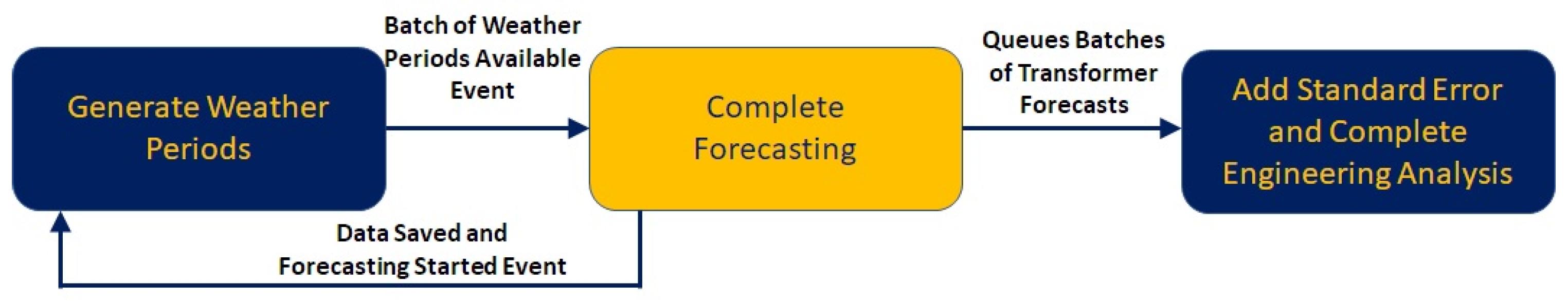
3.1. Overall Structure

To investigate load scenarios that have not yet occurred and the likelihood of those scenarios, the authors sought to efficiently implement Monte Carlo simulations leveraging the forecasting method described in [1]. To reduce the total time to complete the Monte Carlo simulation, a multithreaded and object-oriented approach was implemented by the authors to strategically make use of system resources, specifically the Central Processing Unit (CPU) and Graphics Processing Unit (GPU). The structure to generate the Monte Carlo simulations is shown in Figure 2. This structure will be explained in the following sections.

3.2. Generate Weather Periods

The purpose of the Generate Weather Periods component is to create the weather scenarios needed for the Monte Carlo simulations. The Generate Weather Periods component runs in a dedicated thread on the CPU, and it is triggered to start creating a new batch of data by a Forecasting Started Event from the Complete Forecasting component. A Forecasting Started Event is artificially generated during initialization to start the process. The Generate Weather Periods component generates the weather scenarios over several iterations, with each iteration creating a batch of data to be sent to the next component to create electrical load profiles. This approach of creating batches of data reduces the overall time by allowing downstream components to begin processing data in parallel with the Generate Weather Periods component. In the authors’ preferred configuration, five iterations with batch sizes of 50, 200, 250, 250, and 250 were completed to generate 1000 scenarios for the test periods for Areas 1 and 2 separately.

3.2.1. Batches of Weather Days

After it is triggered to create a batch of weather data, the first step for the Generate Weather Periods component is to use Markov Chains to create a series of day-types for the period being investigated, as illustrated in Figure 3. The random walk requires a serialized processing approach.
The result of this step is shown in Equation (1). The day-type matrices (DT) provide the sequence of day-types to be used in this study. DTTrain is just the historical classification of the weather actually experienced. DTTest is the created sequence of days based on the Markov Chains and will be used to perform the Monte Carlo simulations.
D T T r a i n     d t 0 , 1 d t 0 , H     D a y T y p e s   f o r   T r a i n i n g   P e r i o d   D T T e s t     d t 1 , 1 d t 1 , M d t N , 1 d t N , M   D a y T y p e s   f o r   T e s t i n g   P e r i o d   d t i , j     d a y t y p e   f o r   b a t c h   i ,   d a y   j   N   B a t c h   S i z e   H N u m b e r   o f   D a y s   i n   T r a i n i n g   P e r i o d   M N u m b e r   o f   D a y s   i n   T e s t i n g   P e r i o d  

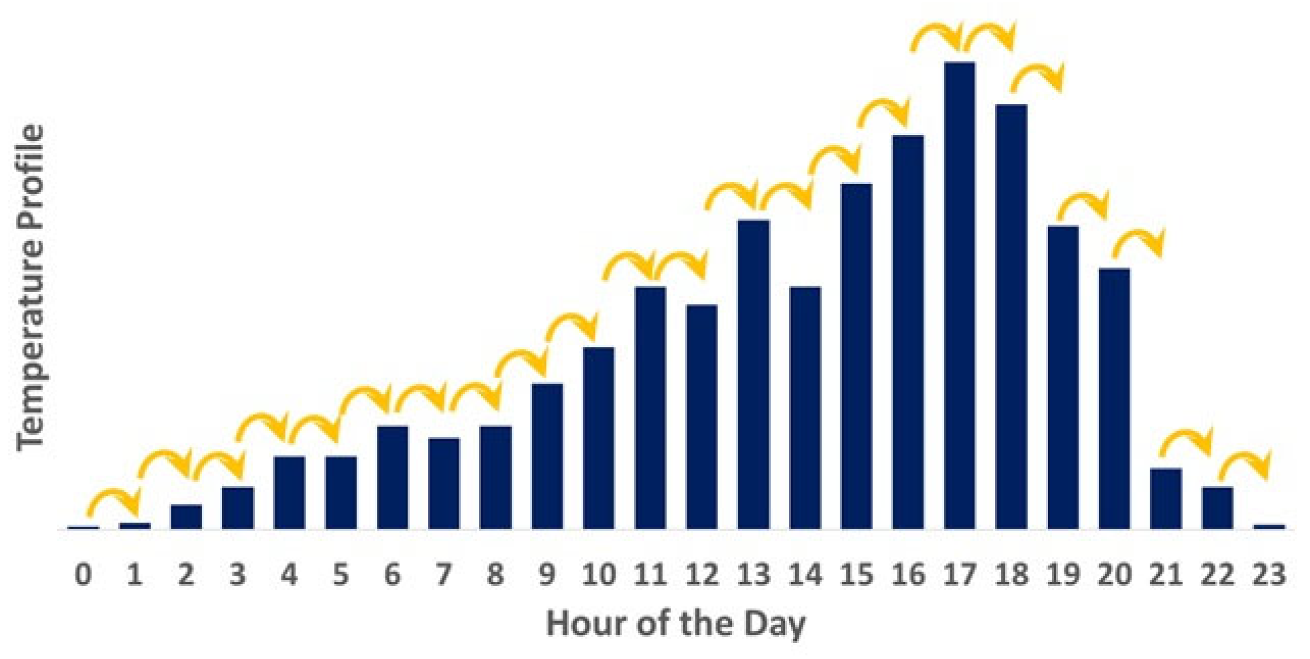
3.2.2. Detailed Weather Profiles

With the sequence of day-types developed, the next step for the Generate Weather Periods component is to use an autoregressive model to create hourly solar, dew point, and temperature profiles for each day in the test period for each simulation, as illustrated in Figure 4. This step has been vectorized for faster processing.
The result of this step is shown in Equation (2). The weather matrices (W) provide the weather data (24 h solar irradiance, temperature, and dew point profiles) to be used in future steps. Again, WTrain is just the historical weather actually experienced, and WTest is the result of the autoregressive model.
W T r a i n     s 0 , 1 , 1 s 0 , 1 , 24   t 0 , 1 , 1 t 0 , 1 , 24   d 0 , 1 , 1 d 0 , 1 , 24 s 0 , H , 1 s 0 , H , 24   t 0 , H , 1 t 0 , H , 24   d 0 , H , 1 d 0 , H , 24 W T e s t s 1 , 1 , 1 s 1 , 1 , 24   t 1 , 1 , 1 t 1 , 1 , 24   d 1 , 1 , 1 d 1 , 1 , 24 s 1 , M , 1 s 1 , M , 24   t 1 , M , 1 t 1 , M , 24   d 1 , M , 1 d 1 , M , 24 s N , 1 , 1 s N , 1 , 24   t N , 1 , 1 t N , 1 , 24   d N , 1 , 1 d N , 1 , 24 s N , M , 1 s N , M , 24   t N , M , 1 t N , M , 24   d N , M , 1 d N , M , 24 s i , j , k     s o l a r   i r r a d i a n c e   f o r   b a t c h   i ,   d a y   j ,   a n d   h o u r   k     t i , j , k     t e m p e r a t u r e   f o r   b a t c h   i ,   d a y   j ,   a n d   h o u r   k     d i , j , k     d e w   p o i n t   f o r   b a t c h   i ,   d a y   j ,   a n d   h o u r   k    

3.2.3. Final Processing

The final step for the Generate Weather Periods component is to complete the final processing of the data to produce a tensor to be sent to the next component. This step is also vectorized for faster processing and creates a tensor for each day in the test period for each simulation. The tensor contains the date, iteration number, batch, month, day of month, current day cluster, next day cluster, day of year, hourly solar profile, hourly temperature profile, hourly dew point profile, day of year sine and cosine representation, weekend, holiday, holiday week, period (i.e., 2021S4), season (S1 to S4), and a period index (1 to 10).

3.3. Complete Forecasting

With the weather scenarios from the Generate Weather Periods component, the Complete Forecasting component implements the forecasting algorithm described in [1]. It generates the stochastic electrical load forecasts needed for the Engineering Analysis that will be described in Section 4. It runs in a dedicated thread on the GPU and is triggered by a Generate Weather Batch Complete Event.

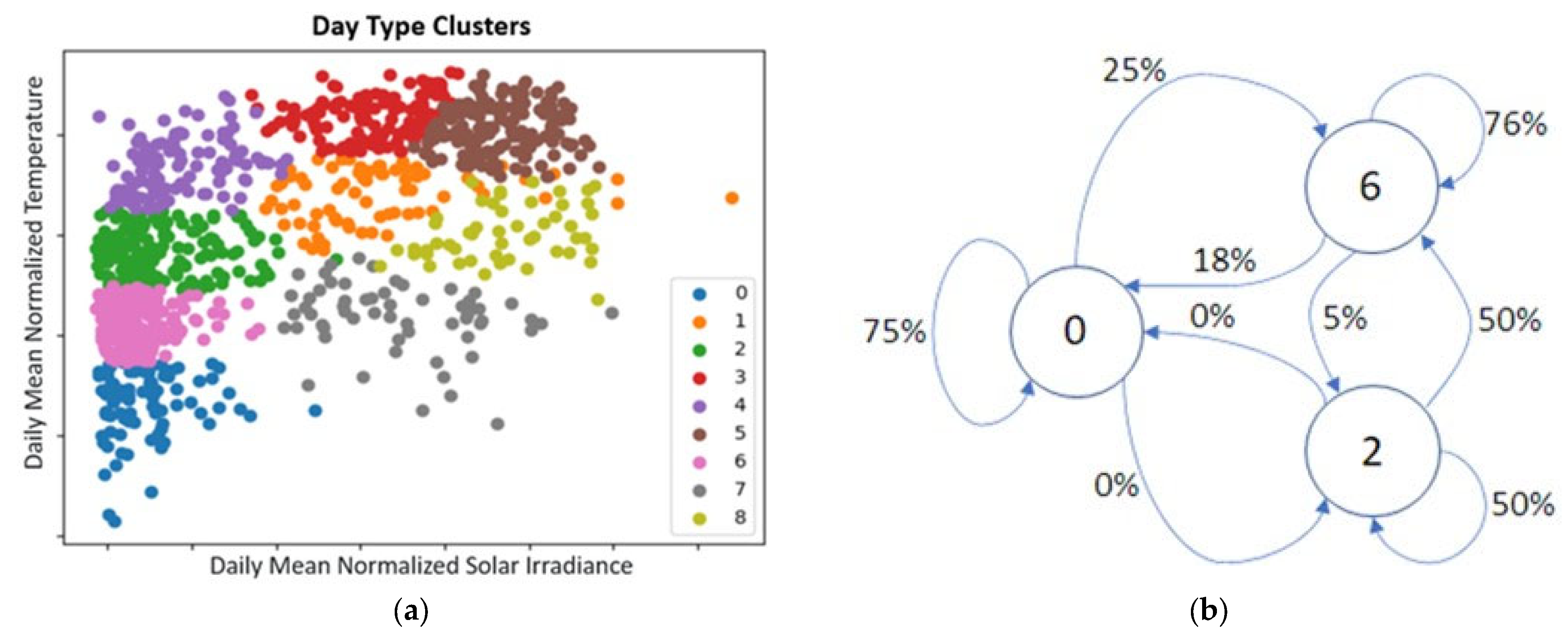
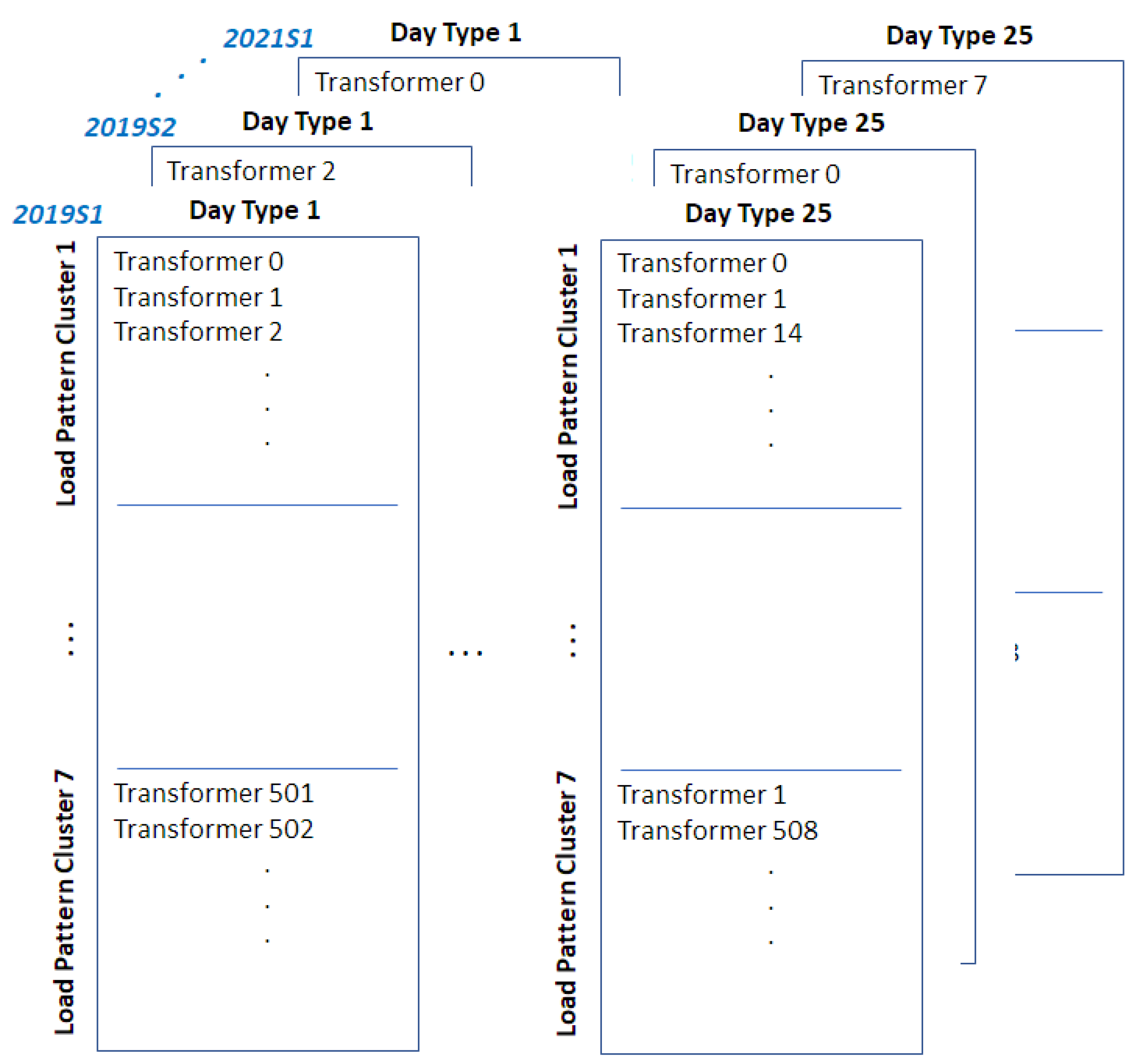
3.3.1. Clustering Forecast

The first step of the Complete Forecasting component is to complete the clustering-based forecasting described in [1], which is illustrated in Figure 5. The result is the Transformer Load Matrix (TLM), which includes key information, such as the initial load forecast for each transformer. It is completed for the entire batch for each transformer provided by the Generate Weather Periods component. This step has been vectorized for each transformer for the entire batch for faster processing.

3.3.2. Prepare Tensor

This step generates a tensor based on the results of the clustering step to feed into the neural network in the next step. It does this for the entire batch for each transformer. This step has been vectorized for each transformer for the entire batch for faster processing and produces a tensor for each transformer for a day in each simulation. It contains day of year sine and cosine representation, transformer data (type, index, relative rating, and z-score for number of customers), day cluster, load cluster, day of year, weekend, holiday, holiday week, season period index (1 to 10), clustering forecast (24 h), hourly solar profile (24 h), hourly temperature profile (24 h), hourly dew point profile (24 h), hourly attention (24 h), and hourly sine and cosine representation (24 h).

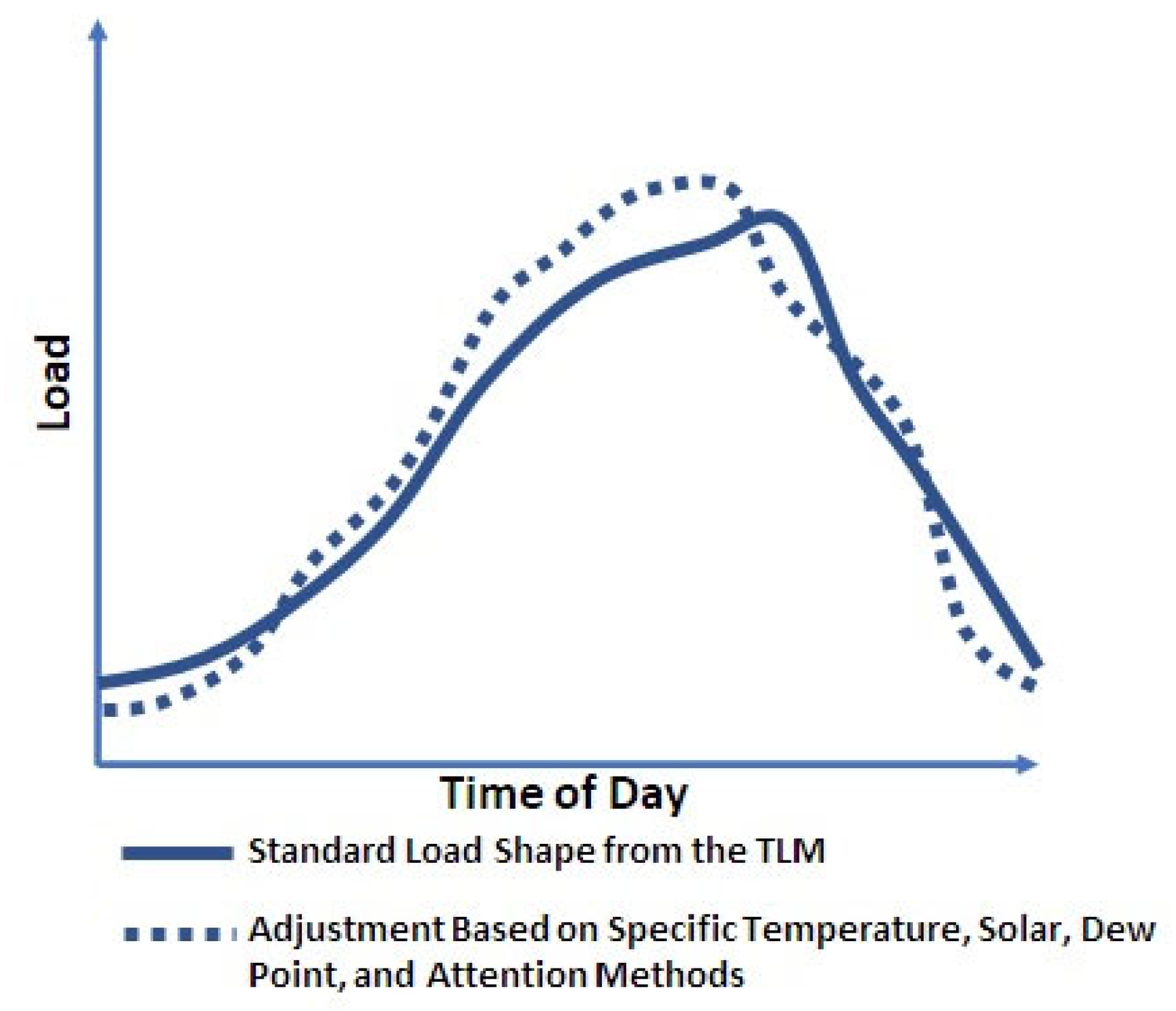
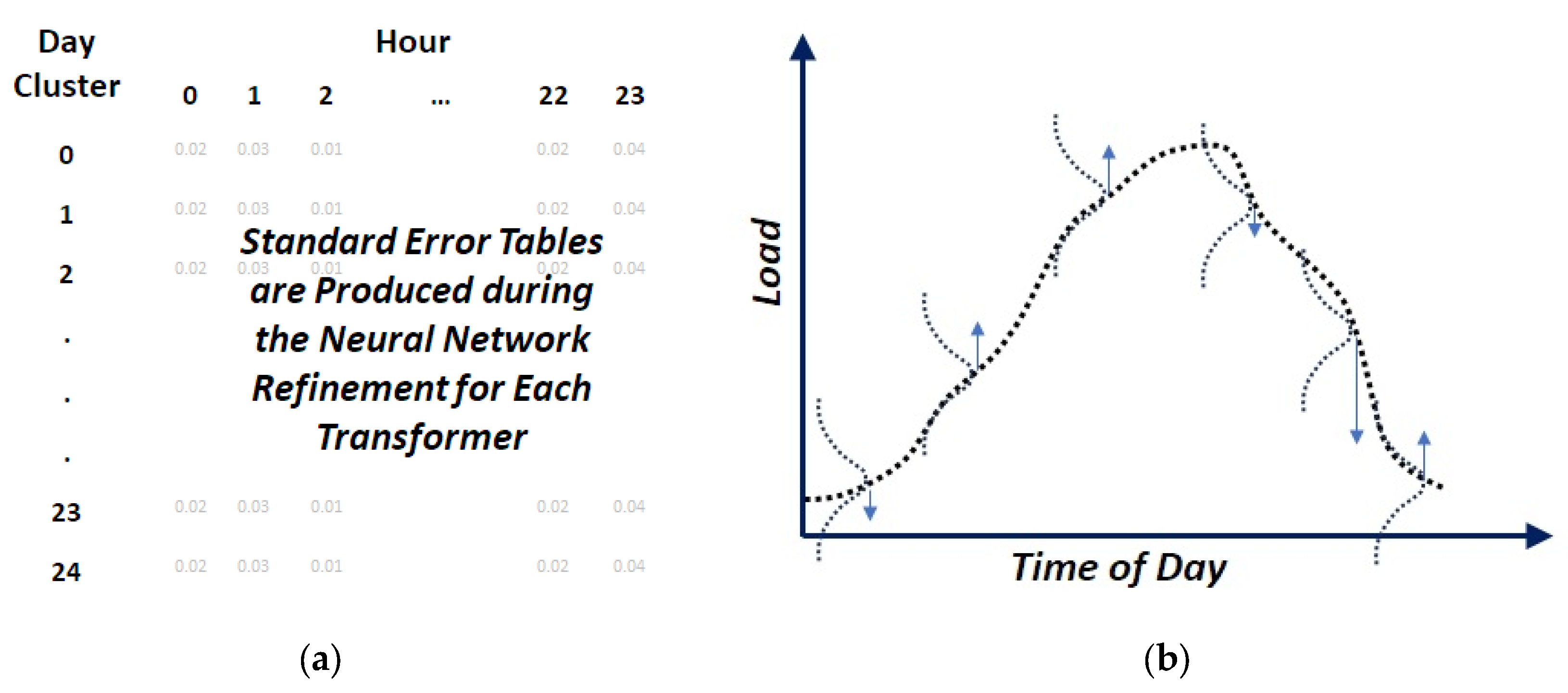
3.3.3. Neural Network Refinement

The final step of the Complete Forecasting component is to implement the Neural Network Refinement element described in [1] and illustrated in Figure 6. It is completed for the entire batch for each transformer. This step has been vectorized for each transformer for the entire batch for faster processing.

3.4. Add Standard Error and Implement Engineering Analysis

Regression models typically include a standard error that considers the model’s fit to the training data. To consider this, a standard error table is created for each transformer during the neural network training, as described in [1]. The results from the Complete Forecasting component are the expected value of the forecasting model. Additional variation can be expected based on the standard error table. This is considered by first completing a random sampling within the standard error distribution. This result is then added to the expected value of the forecast to provide the final forecast to be used in Engineering Analysis [37]. This is illustrated in Figure 7. The results are used in the Engineering Analysis that will be described in Section 4. This component runs in a dedicated thread running on the CPU, and it queues data from the Complete Forecasting component.
The result of this step is shown in Equation (3). The load matrices (L) are created for each transformer, which will be used in Engineering Analysis. LTrain is the actual load experienced by the transformer, and LTest is the forecasted load for each of the Monte Carlo simulations.
L T r a i n     l 0 , 1 , 1 l 0 , 1 , 24 l 0 , H , 1 l 0 , H , 24 L T e s t     l 1 , 1 , 1 l 1 , 1 , 24 l 1 , M , 1   l 1 , M , 24 l N , 1 , 1 l N , 1 , 24 l N , M , 1   l N , M , 24 l i , j , k     l o a d   f o r   b a t c h   i ,   d a y   j ,   a n d   h o u r   k

4. Engineering Analysis

Reference [1] contemplated use cases for the Monte Carlo simulations, but it did not develop those use cases. This section describes how the results of the Monte Carlo simulations can be used. While there are many use cases, the authors prioritized proactively identifying and correcting concerns that can impact customers. This section describes two uses that the authors have developed: Transformer Failures due to Loading and Power Quality Concern Prediction.
The tools provided by [38,39,40,41,42] were helpful in the Monte Carlo and Engineering Analysis, with [38] providing the method to complete the forecast training and prediction on the GPU [39,40], providing the means to read and process the data, and [41,42] provide data analysis tools that ran on the CPU and GPU respectively.

4.1. Transformer Failures Due to Loading

IEEE Standard C57.91-2011 can be used to determine the loss of transformer life due to load [24,43]. As described in IEEE Standard C57.91-2011, insulation deterioration is a key component of transformer life, and insulation deterioration is a function of time, moisture content, oxygen content, and temperature. With modern construction techniques, moisture and oxygen content can be minimized, which leaves temperature as the primary controllable factor.

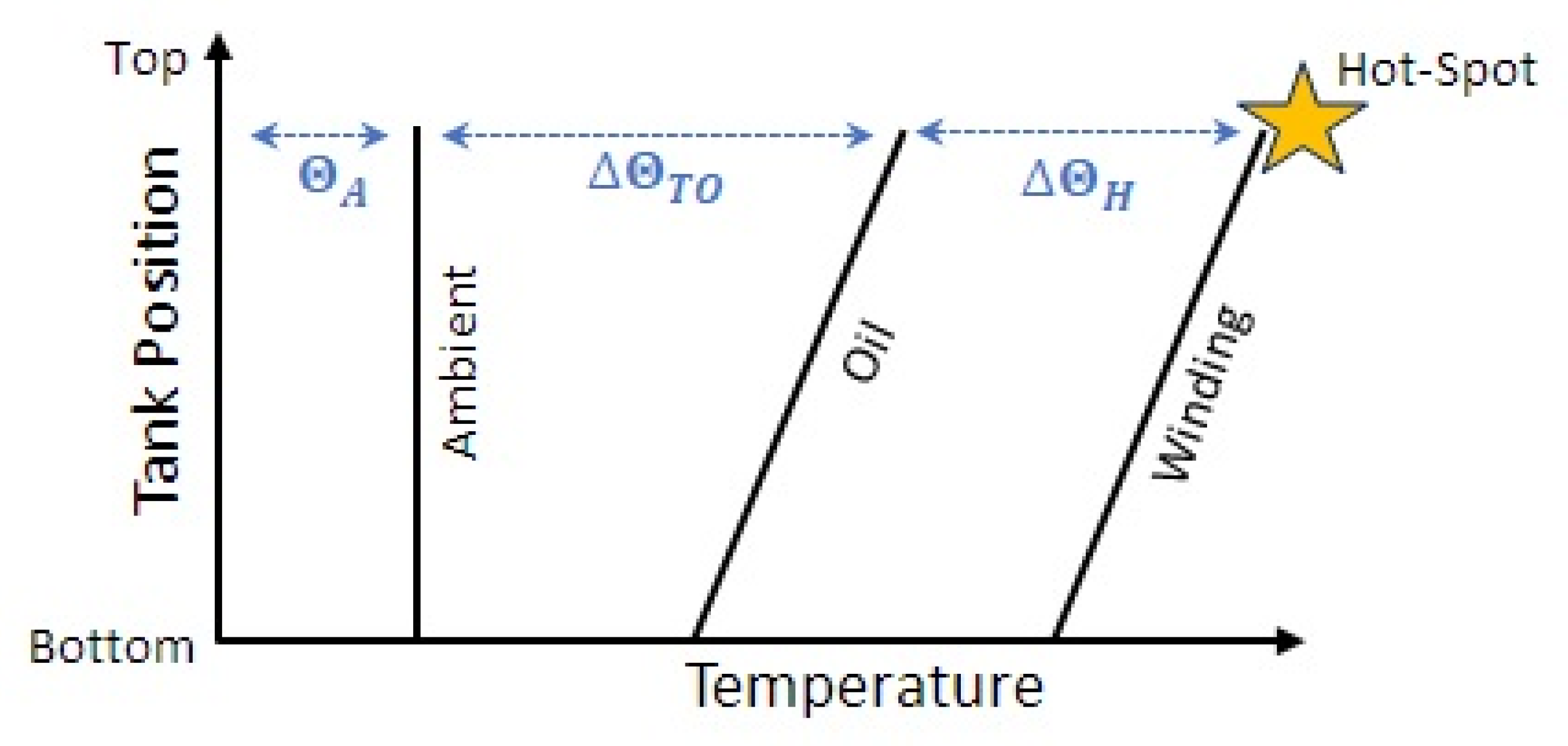
4.1.1. Hot-Spot Determination

Figure 8 illustrates the determination of the highest insulation temperature (Hot-Spot). The Hot-Spot will most likely be on the transformer windings at the top of the transformer tank and will be the summation of the ambient temperature, oil temperature, and winding temperature. The authors used this standard with the load forecasts from the Monte Carlo simulations to determine the likelihood of a transformer failure due to loading.
The standard provides guidance on determining each of these temperatures based on the transformer’s load.
The top oil temperature rise over ambient temperature is determined using the following:
Δ Θ T O , i = Δ Θ T O , R ( K i 2 R + 1 ) R + 1 n Δ Θ T O , U = Δ Θ T O , R ( K U 2 R + 1 ) R + 1 n Δ Θ T O = Δ Θ T O , U Δ Θ T O , i   1 e t / τ T O + Δ Θ T O , i Θ T O T o p O i l   T e m p e r a t u r e   ° C Δ Θ T O   T o p O i l   R i s e   O v e r   A m b i e n t   ° C Δ Θ T O , R   T o p O i l   R i s e   O v e r   A m b i e n t   a t   R a t e d   L o a d   ° C Δ Θ T O , i   I n i t i a l   T o p O i l   R i s e   O v e r   A m b i e n t   ° C Δ Θ T O , U   U l t i m a t e   T o p O i l   R i s e   O v e r   A m b i e n t   ° C τ T O   O i l   T i m e   C o n s t a n t K i   R a t i o   o f   I n i t i a l   L o a d   t o   R a t e d   L o a d K U   R a t i o   o f   U l t i m a t e   L o a d   t o   R a t e d   L o a d R   R a t i o   o f   L o a d   L o s s   a t   R a t e d   L o a d   t o   N o   L o a d   L o s s n   E m p e r i c a l l y   D e r i v e d   E x p o n e n t  
The winding Hot-Spot temperature relative to the top oil temperature is calculated using the following equations.
Δ Θ H , i = Δ Θ H , R K i 2 m Δ Θ H , U = Δ Θ H , R K U 2 m Δ Θ H = Δ Θ H , U Δ Θ H , i   1 e t / τ W + Δ Θ H , i Θ H W i n d i n g   H o t t e s t S p o t   T e m p e r a t u r e   ° C Δ Θ H   W i n d i n g   H o t t e s t S p o t   T e m p e r a t u r e   O v e r   T o p   O i l   ° C Δ Θ H , R   W i n d i n g   H o t t e s t S p o t   T e m p e r a t u r e   O v e r   T o p   O i l   a t   R a t e d   L o a d   ° C Δ Θ H , i   I n i t i a l   W i n d i n g   H o t t e s t S p o t   T e m p e r a t u r e   O v e r   T o p   O i l   ° C Δ Θ H , U   U l t i m a t e   W i n d i n g   H o t t e s t S p o t   T e m p e r a t u r e   O v e r   T o p   O i l   ° C τ W   W i n d i n g   T i m e   C o n s t a n t m   E m p e r i c a l l y   D e r i v e d   E x p o n e n t  
With the top oil temperature and winding Hot-Spot temperatures, the impact on transformer life can be determined using the following:
Θ H = Θ A   + Δ Θ T O + Δ Θ H F A A = e 15000 383 15000 Θ H + 273 F E Q A = n = 1 N F A A , n   Δ t n n = 1 N   Δ t n % l o s s   o f   l i f e = F E Q A   x   t   x   100 N o r m a l   I n s u l a t i o n   L i f e Θ H W i n d i n g   H o t t e s t S p o t   T e m p e r a t u r e   ° C Θ A A v e r a g e   A m b i e n t   T e m p e r a t u r e   ° C F A A   A g i n g   A c c e l e r a t i o n   F a c t o r   f o r   a   P e r i o d F A A , n   A g i n g   A c c e l e r a t i o n   F a c t o r   f o r   P e r i o d   n F E Q A   A c c u m u l a t e d   A g i n g   F a c t o r  

4.1.2. Transformer Thermal Parameters

Some of the parameters required for the implementation of IEEE Standard C57.91-2011 are available in the standard, such as m and n. Others must be determined through testing. Because the distribution transformers installed on the electrical distribution system vary based on many factors, including their installation date, past usage, manufacturer, manufacturing date, and many others, determining the transformer parameters needed for the calculations is a challenge for a wide-scale application of IEEE Standard C57.91-2011. To address this issue, the authors established a range of parameters to use based on discussions with transformer manufacturers and industry experts, as shown in Table 1. Note that there can be wider variation in these parameters, including with newer, more efficient transformer designs. The results are determined for the range of parameters to determine their impact on the Hot-Spot calculations, which is presented in Section 5.1.2 and shows that they provided beneficial outcomes. Specifically, the “Mid” set of values applied for a wide-scale application of IEEE Standard C57.91-2011 provided good results in this study.

4.1.3. Implementation Details

To implement the calculations described in Equations (4)–(6) using the values in Table 1, the first event records were analyzed to determine the last time each transformer in the study was replaced. The date and time for that event is the starting point for the calculation using the historical load for each transformer (LTrain) from Equation (3). Those data were then coupled with the forecasted load for each transformer for all the simulations (LTest) from Equation (3). The consolidated data were then sequentially processed from hour to hour through Equations (4)–(6). The result is the remaining useful life for each transformer for each Monte Carlo simulation. The portion of the Monte Carlo simulations ending with 100% or greater of the useful life being exhausted is the likelihood of failure.

4.2. Power Quality Concern Prediction

In addition to using the Monte Carlo simulations for transformer failure predictions, the authors sought to also use them to identify and address power quality events before they were experienced by customers. Power quality events, in this case, are defined as low voltage, high voltage, and flicker events reported by customers.

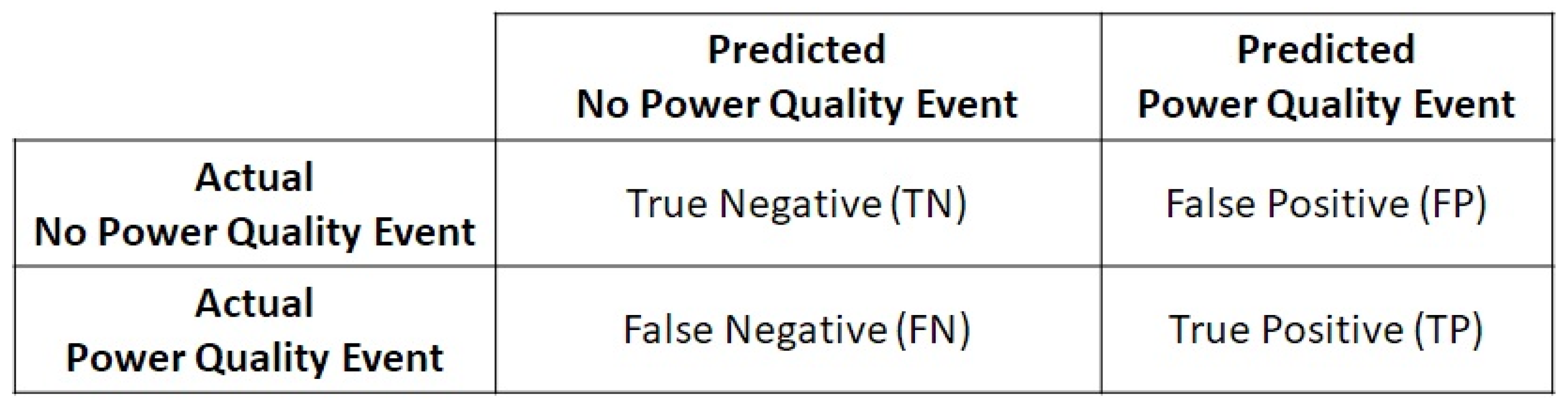
4.2.1. Classification Evaluation

The authors reviewed the work in [44,45] to develop measures and analysis methods for evaluating the classification models with a range of hyperparameters.
The confusion matrix shown in Figure 9 was used in this study.
The key metrics used in this study are defined in Equation (7) based on the confusion matrix shown in Figure 9. Accuracy (A) will be a key measure to evaluate the overall results of the power quality event classification model. True Positive Rate (TPR) measures the number of actual power quality events predicted to the total number of power quality events experienced by customers. A high TPR value indicates that a high number of power quality events can be identified and addressed before they are realized by customers. Thus, TPR is a measure of the model’s focus on customer service. On the other hand, Precision Rate (P) is a measure of how many transformers predicted to experience power quality concerns actually have power quality concerns. Each one of these transformers will have to be investigated by engineers and field crews. A high p-value indicates that a high ratio of transformers being investigated will actually have issues. Thus, it is a measure focused on efficiency. Finding the right balance between these three measures is part of the overall objective.
A c c u r a c y   A     T P + T N T P + T N + F P + F N T r u e   P o s i t i v e   R a t e   T P R     T P T P + F N P r e c i s i o n   R a t e   P     T P T P + F P

4.2.2. Classification Model

The authors experimented with several feature sets derived from the Monte Carlo simulations, several classification models, and different values of hyperparameters for the classification models to predict power quality events during the period under investigation (test periods for Areas 1 and 2). The classifier was trained using the training periods for Areas 1 and 2 separately. The predicted power quality events were then determined by using the data from the test period and compared to the actual power quality events experienced by customers during that period. A summary of the factors for the experiments is included in Table 2.
To elaborate on Table 2, the features included in the first column are all calculated with the results of the Monte Carlo simulations and defined as follows:
  • Entropy—The differential entropy as defined in [39]
  • Percent Greater than 1—The percentage of hours where the load is greater than the capacity of the transformer
  • Absolute Difference Mean—The average of the difference in load from hour to hour
  • Average—The average of the load in the simulations result
  • Standard Deviation—The standard deviation of the load in the simulations result
  • Maximum—The maximum of the load in the simulations result
  • Minimum—The minimum of the load in the simulations result
The authors attempted to train three different classification models. The results for LR and RF are presented in Section 5.1.3. Attempts to train SVM were also completed, but none of those endeavors provided good results.
There are many hyperparameters for each classification model (see the Nomenclature section and [46,47,48] for more details). The authors investigated variation in many and reviewed research [44,45] to determine the most impactful hyperparameters, which are listed in the third column of Table 2. Values for these hyperparameters were selected, and adjustments were made to determine the results. Those results are provided in Section 5.1.3.
A few hyperparameters require additional explanation. The true samples are weighted because false samples are disproportionately high (i.e., there are far fewer transformers experiencing power quality events than those that do not experience power quality events. Also, the classifier threshold uses the average of the probabilities of true classification across all simulations to determine the final classification based on the defined threshold.

4.2.3. Implementation Details

The features for each transformer, which are described in Section 4.2.2, are calculated using the load results for each transformer (LTrain and LTest), which is described in Equation (3). The features determined with the training period load values from each transformer (LTrain) are used as inputs to the classification model, with the desired outputs being power quality events realized during the training period. This trained model is then tested with the feature sets derived from test period forecasted load data (LTest) from Equation (3). The threshold previously described was used to determine the classification for each transformer, and those classifications were compared to actual power quality events experienced during the test period to determine the efficacy of the model.

5. Research Findings and Future Work

The research findings and how they will lead to future work are presented in this section.

5.1. Research Findings

The research findings can be considered in three categories—(1) the time to complete the Monte Carlo simulations and the time to complete the overall process, (2) the efficacy of the transformer failure results, and (3) the efficacy of the power quality predictions.

5.1.1. Monte Carlo Results

The structure described in Section 3 produced 1000 simulations for approximately four months from July 2021 to early November 2021 for 389 transformers in Area 1 in approximately 44 min and for five months from July 2021 to early December 2021 for 454 transformers in Area 2 in approximately 55 min. The time to complete the Engineering Analysis described in Section 4 is 11 min for Area 1 and 15 min for Area 2. When added to the training times in Table 2 from [1], the overall process can be completed in approximately 103 to 118 min for 389 to 454 transformers (approximately 48 million to 69 million points), respectively.
The work was completed on a system with the following specifications: CPU: AMD Ryzen 7 5800X with 3801 MHz Default Clock Speed, GPU: NVIDIA GeForce RTX 3060 Ti, RAM: 4 X G. Skill F4-3200C16-16GVK DD4 for 64 GB, Motherboard: HP 8876.

5.1.2. Transformer Failure Results

The Monte Carlo simulations were used with the guidance from IEEE Standard C57.91-2011 to predict transformer failures, and the results were compared with actual failures in the period under investigation (test periods for Areas 1 and 2). The results are shown in Table 3, with the Transformer Index defined as a unique index for each transformer in the study. The Percentage of Monte Carlo Simulations that Exceeded 100% Useful Life is the percentage of the 1000 simulations that ended greater than 100. This calculation uses the percentage loss of life determined through the implementation of IEEE Standard C57.91-2011 for the training and test periods for all the 1000 Monte Carlo simulations and each set of transformer parameters defined in Section 4.1. Finally, Transformer Outage Events are the actual transformer outage events experienced during the period under investigation (test periods for Areas 1 and 2). All the transformers in Table 3 were considered likely to fail during the test period.
As shown in Table 3, four of the ten transformers predicted to be most likely to fail did fail during the period under investigation. Initially, transformers 385, 475, 286, 480, and 389 all showed some percentage of the 1000 simulations ending with 100% of the useful life being exceeded for some scenarios. None of these five transformers experienced an actual transformer outage event, but field investigations led to the identification of transformer capacity data issues. After the data were improved, 0% of the simulations ended with 100% of the useful life being exceeded. Similarly, AMI voltage correlation and meter-to-transformer distance analysis showed that transformer 275 had over 56% more customers mapped to it than was actually the case. Identifying these issues through this method allowed for these data to be improved, and the results are summarized in the Data Improvement Opportunity Identified column in Table 3.
It can also be seen from Table 3 that variation in the transformer thermal parameters needed for the implementation of IEEE Standard C57.91-2011 leads to different values. However, it shows that the top predicted transformer failures do not vary significantly.

5.1.3. Power Quality Event Predictions

Table 4 and Table 5 show the results of the power quality event prediction experiments to determine the proper balance between accuracy, customer service, and efficiency measures.
The authors found the bold line in Table 4 as the best option. The bold line in Table 4 would have led to proactively identifying six transformers with power quality issues out of the 835 transformers that were classified. This model would have required the investigation of 56 transformers; 25 transformers actually had power quality concerns during the period under investigation.
The LR results presented in Table 5 show that accuracy did not exceed 67.8% and precision did not exceed 6.1%. Experiments were also completed using SVM, but SVM did not show good results. This led the authors to select RF as the best option for the purpose.
Starting with the bold line in Table 4, a feature ablation study was completed. The results of that study are presented in Table 6.
From the results of the feature ablation study presented in Table 6, removing the “percent greater than 1” variable, which is emphasized with the bold line, slightly improves the results. With this improvement, engineers would have to investigate 54 transformers (i.e., more efficient) with no loss of TPR (i.e., maintaining customer service focus).

5.1.4. Research Findings Summary

The forecasting method described in [1] can be used to efficiently generate stochastic electrical load forecasts. Strategically using CPU and GPU resources and event synchronized threading are critical to reducing the overall time to complete the simulations. One key aspect of efficiently completing the Monte Carlo simulations is to generate batches of the needed input parameters, such as weather data, in one thread, with the batch sizes varying to start the parallel processing in downstream components. Furthermore, vectorizing data processing wherever possible reduces the overall time.
These simulations can be used with IEEE Standard C57.91-2011 to accurately predict transformer failures and to identify data improvement opportunities. The key thermal parameters of transformers can vary widely based on many factors, including installation date, past usage, manufacturer, and manufacturing date. It would at least be difficult, if not impossible, to determine these parameters for all the transformers to be included in a wide-scale implementation of IEEE Standard C57.91-2011; but the work described in this manuscript has shown that transformer failures and data improvement opportunities can be predicted by using a standard mid-range of values. Finally, the simulations can be used with classification models to predict power quality events and provide measures of overall accuracy, true positive rate, and precision to allow utilities to find the proper balance between a focus on customer satisfaction and engineering efficiency. This work has shown that the Random Forest classification method with proper selection of weighting, thresholds, and other hyperparameters performed the best with differential entropy, absolute difference mean, average, standard deviation, maximum, and minimum measures derived from the stochastic electrical load forecasts.

5.1.5. Future Work

The work described in this manuscript and [1] provides a foundation for utilities to prevent customers from experiencing outage and non-outage events with the evolving electrical distribution system. While this work has provided some meaningful contributions, time constraints have led to two limitations: the authors believe the overall method described in [1] can be further developed and verified, and the scope of the Engineering Analysis can be expanded past distribution transformers.
With the foundation that has been established and considering the limitations, the authors plan to expand their work in four directions. First, there will be a focus on improving the overall accuracy and predicting capability of the method described in [1]. Second, the work will be expanded past the original datasets to other geographic areas and time periods to both test and further develop it. Third, the work described in this manuscript will be expanded to additional Engineering Analysis, including aggregating the results to anticipate protection concerns and the risk of equipment damage beyond distribution transformers. The aggregated results also have the potential to identify areas with lightly loaded equipment, which can lead to ferroresonance risk [49,50,51]. Finally, the authors plan to use these new methods to consider new opportunities for electric utilities, including the use of non-wires alternatives (NWAs), microgrid technology, and adaptive networked microgrids (ANMs).

Author Contributions

Conceptualization, J.O.; methodology, J.O.; software, J.O.; validation, J.O.; formal analysis, J.O.; investigation, J.O.; resources, J.O.; data curation, J.O.; writing—original draft preparation, J.O.; writing—review and editing, W.S.; visualization, J.O.; supervision, W.S.; project administration, J.O.; funding acquisition, J.O. and W.S. All authors have read and agreed to the published version of the manuscript.

Funding

This research received no external funding.

Data Availability Statement

The data and electrical system configurations used in this research are confidential. The code and results are available.

Acknowledgments

The authors wish to thank Angela Leigl and Albert Penner from Eaton Corporation and Hamza Kakakhel from DTE Electric for providing guidance on the transformer data needed for the application of IEEE Standard C57.91-2011. The authors also wish to thank Fernando Duarte from The Electric Power Research Institute (EPRI) for providing guidance on the application of IEEE Standard C57.91-2011. Finally, the authors would like to thank Alex Little from DTE Electric for his work to confirm the number of customers mapped to transformer 275.

Conflicts of Interest

The authors declare no conflict of interest.

Nomenclature

AAccuracy
AMIAutomated Meter Infrastructure
ANMAdaptive Networked Microgrid
CMACumulative Moving Average
CPUCentral Processing Unit
DERDistributed Energy Resources
EPRIElectric Power Research Institute
ERCOTElectric Reliability Council of Texas
EVElectric vehicles
GPUGraphics Processing Unit
LRLogistic Regression
LTFLong-Term Forecast
MTFMedium-Term Forecasts
PPrecision
PEAProvincial Electricity Authority of Thailand
RFRandom Forest
STFShort-Term Forecast
SVMSupport Vector Machine
TPRTrue Positive Rate
VSTFVery-Short-Term Forecast
Training PeriodJuly 2019 to June 2021
Training DataData from the Training Period not included in the Validation Data
Validation DataRandomly selected 10% of data from Training Period
Test Period Area 1July 2021 to November 2021
Test Period Area 2July 2021 to December 2021
Period Under InvestigationTest Periods for Area 1 and Area 2
D T T r a i n D a y T y p e s   f o r   T r a i n i n g   P e r i o d
D T T e s t D a y T y p e s   f o r   T e s t i n g   P e r i o d
d t i , j   d a y t y p e   f o r   b a t c h   i ,   d a y   j
N B a t c h   S i z e
H N u m b e r   o f   D a y s   i n   T r a i n i n g   P e r i o d
M N u m b e r   o f   D a y s   i n   T e s t i n g   P e r i o d
W T r a i n W e a t h e r   M a t r i x   f o r   t h e   T r a i n i n g   P e r i o d
W T e s t W e a t h e r   M a t r i x   f o r   t h e   T e s t i n g   P e r i o d
s i , j , k   s o l a r   i r r a d i a n c e   f o r   b a t c h   i ,   d a y   j ,   a n d   h o u r   k
t i , j , k   t e m p e r a t u r e   f o r   b a t c h   i ,   d a y   j ,   a n d   h o u r   k
d i , j , k   d e w   p o i n t   f o r   b a t c h   i ,   d a y   j ,   a n d   h o u r   k
L T r a i n L o a d   f o r   t h e   T r a i n i n g   P e r i o d
L T e s t L o a d   f o r   t h e   T e s t i n g   P e r i o d
l i , j , k   l o a d   f o r   b a t c h   i ,   d a y   j ,   a n d   h o u r   k
Parameters Used with IEEE Standard C57.91-2011
Θ TO Top Oil   Temperature   ° C
Δ Θ TO Top Oil   Rise   Over   Ambient   ° C
Δ Θ TO , R Top     Oil   Rise   Over   Ambient   at   Rated   Load   ° C
Δ Θ TO , i Initial   Top Oil   Rise   Over   Ambient   ° C
Δ Θ TO , U Ultimate   Top Oil   Rise   Over   Ambient   ° C
τ TO   Oil   Time   Constant
K i   Ratio   of   Initial   Load   to   Rated   Load
K U   Ratio   of   Ultimate   Load   to   Rated   Load
R Ratio   of   Load   Loss   at   Rated   Load   to   No   Load   Loss
n Emperically   Derived   Exponent
Θ H Winding   Hottest Spot   Temperature   ° C
Δ Θ H Winding   Hottest Spot   Temperature   Over   Top   Oil   ° C
Δ Θ H , R Winding   Hottest Spot   Temperature   Over   Top   Oil   at   Rated   Load   ° C
Δ Θ H , i Initial   Winding   Hottest Spot   Temperature   Over   Top   Oil   ° C
Δ Θ H , U Ultimate   Winding   Hottest Spot   Temperature   Over   Top   Oil   ° C
τ W   Winding   Time   Constant
m Emperically   Derived   Exponent
Hyperparameters Used with Classifiers
CUsed with SVM and LR—Regularization parameter. The strength of the regularization is inversely proportional to C [46,48]
GammaUsed with SVM—Kernel coefficient [46]
Max DepthUsed with RF—The maximum depth of the tree [47]
Minimum Samples per LeafUsed with RF—The minimum number of samples required to be at a leaf node [47]
Classifier ThresholdUsed with All—The threshold for deciding between two classifications.
Category WeightsUsed with All—A weighting applied to samples that are disproportionately distributed

References

  1. O’Donnell, J.; Su, W. Attention-Focused Machine Learning Method to Provide the Stochastic Load Forecasts Needed by Electric Utilities for the Evolving Electrical Distribution System. Energies 2023, 16, 5661. [Google Scholar] [CrossRef]
  2. Pinheiro, M.G.; Madeira, S.C.; Francisco, A.P. Short-Term Electricity Load Forecasting—A Systematic Approach from System Level to Secondary Substations. Appl. Energy 2023, 332, 120493. [Google Scholar] [CrossRef]
  3. Farsi, B.; Amayri, M.; Bouguila, N.; Eicker, U. On Short-Term Load Forecasting Using Machine Learning Techniques and a Novel Parallel Deep LSTM-CNN Approach. IEEE Access 2021, 9, 31191–31212. [Google Scholar] [CrossRef]
  4. L’Heureux, A.; Grolinger, K.; Capretz, M.A.M. Transformer-Based Model for Electrical Load Forecasting. Energies 2022, 15, 4993. [Google Scholar] [CrossRef]
  5. Agarwal, K.; Dheekollu, L.; Dhama, G.; Arora, A.; Asthana, S.; Bhowmik, T. Deep Learning Based Time Series Forecasting. In Proceedings of the 2020 19th IEEE International Conference on Machine Learning and Applications (ICMLA), IEEE, Miami, FL, USA, 14–17 December 2020; pp. 859–864. [Google Scholar] [CrossRef]
  6. Wang, J.; Liu, H.; Zheng, G.; Li, Y.; Yin, S. Short-Term Load Forecasting Based on Outlier Correction, Decomposition, and Ensemble Reinforcement Learning. Energies 2023, 16, 4401. [Google Scholar] [CrossRef]
  7. Guo, J.; Zhang, Z.; Gao, W.; Hu, H.; Wang, D.; Mao, Y. Overheating Risk Warning Model Based on Thermal Circuit Model and Load Forecasting for Distribution Transformers. In Proceedings of the 2019 IEEE Sustainable Power and Energy Conference (iSPEC), Beijing, China, 21–23 November 2019; pp. 2891–2895. [Google Scholar] [CrossRef]
  8. Alotaibi, M.A. Machine Learning Approach for Short-Term Load Forecasting Using Deep Neural Network. Energies 2022, 15, 6261. [Google Scholar] [CrossRef]
  9. Xu, J. Research on Power Load Forecasting Based on Machine Learning. In Proceedings of the 2020 7th International Forum on Electrical Engineering and Automation (IFEEA), Hefei, China, 25–27 September 2020; pp. 562–567. [Google Scholar] [CrossRef]
  10. Phetsangkat, P.; Chalermyanont, K.; Duangsoithong, R. Hierarchical Clustering Electric Load: Case Study in Lower South Region of Thailand. In Proceedings of the 2019 16th International Conference on Electrical Engineering/Electronics, Computer, Telecommunications and Information Technology (ECTI-CON), Pattaya, Thailand, 10–13 July 2019; pp. 881–884. [Google Scholar] [CrossRef]
  11. Cho, J.; Yoon, Y.; Son, Y.; Kim, H.; Ryu, H.; Jang, G. A Study on Load Forecasting of Distribution Line Based on Ensemble Learning for Mid- to Long-Term Distribution Planning. Energies 2022, 15, 2987. [Google Scholar] [CrossRef]
  12. Bento, P.M.R.; Pombo, J.A.N.; Calado, M.R.A.; Mariano, S.J.P.S. Stacking Ensemble Methodology Using Deep Learning and ARIMA Models for Short-Term Load Forecasting. Energies 2021, 14, 7378. [Google Scholar] [CrossRef]
  13. Han, J.; Yan, L.; Li, Z. A Task-Based Day-Ahead Load Forecasting Model for Stochastic Economic Dispatch. IEEE Trans. Power Syst. 2021, 36, 5294–5304. [Google Scholar] [CrossRef]
  14. Hong, Y.; Zhou, Y.; Li, Q.; Xu, W.; Zheng, X. A Deep Learning Method for Short-Term Residential Load Forecasting in Smart Grid. IEEE Access 2020, 8, 55785–55797. [Google Scholar] [CrossRef]
  15. Wang, B.; Wang, X.; Wang, N.; Javaheri, Z.; Moghadamnejad, N.; Abedi, M. Machine Learning Optimization Model for Reducing the Electricity Loads in Residential Energy Forecasting. Sustain. Comput. Inform. Syst. 2023, 38, 100876. [Google Scholar] [CrossRef]
  16. Park, H.; Baldick, R.; Morton, D.P. A Stochastic Transmission Planning Model With Dependent Load and Wind Forecasts. IEEE Trans. Power Syst. 2015, 30, 3003–3011. [Google Scholar] [CrossRef]
  17. Gong, Q.; Midlam-Mohler, S.; Marano, V.; Rizzoni, G. Study of PEV Charging on Residential Distribution Transformer Life. IEEE Trans. Smart Grid 2012, 3, 404–412. [Google Scholar] [CrossRef]
  18. Guoliang, W.; Yuan, H.; Wen, Z.; Junyong, L.; Kangkang, W. Stochastic Optimization of a Microgrid Considering Classification of Electric Vehicles. In Proceedings of the 2023 Panda Forum on Power and Energy (PandaFPE), Chengdu, China, 27–30 April 2023; pp. 2323–2329. [Google Scholar] [CrossRef]
  19. Fan, V.H.; Meng, K.; Dong, Z. Stochastic Electric Vehicle Charging Optimization in Distribution Network. In Proceedings of the 2021 6th Asia Conference on Power and Electrical Engineering (ACPEE), Chongqing, China, 8–11 April 2021; pp. 693–697. [Google Scholar] [CrossRef]
  20. Liu, J.; Shen, H.; Yang, F. Reliability Evaluation of Distribution Network Power Supply Based on Improved Sampling Monte Carlo Method. In Proceedings of the 2020 5th Asia Conference on Power and Electrical Engineering (ACPEE), Chengdu, China, 4–7 June 2020; pp. 1725–1729. [Google Scholar] [CrossRef]
  21. Aprillia, H.; Yang, H.-T.; Huang, C.-M. Statistical Load Forecasting Using Optimal Quantile Regression Random Forest and Risk Assessment Index. IEEE Trans. Smart Grid 2021, 12, 1467–1480. [Google Scholar] [CrossRef]
  22. Giannelos, S.; Borozan, S.; Strbac, G. A Backwards Induction Framework for Quantifying the Option Value of Smart Charging of Electric Vehicles and the Risk of Stranded Assets under Uncertainty. Energies 2022, 15, 3334. [Google Scholar] [CrossRef]
  23. Dong, M.; Nassif, A.B.; Li, B. A Data-Driven Residential Transformer Overloading Risk Assessment Method. IEEE Trans. Power Deliv. 2019, 34, 387–396. [Google Scholar] [CrossRef]
  24. C5791-2011; IEEE Guide for Loading Mineral-Oil-Immersed Transformers and Step-Voltage Regulators. Revised IEEE Standard C5791-1995. IEEE: New York, NY, USA, 2012; pp. 1–123. [CrossRef]
  25. Sönmez, O.; Komurgoz, G. Determination of Hot-Spot Temperature for ONAN Distribution Transformers with Dynamic Thermal Modelling. In Proceedings of the 2018 Condition Monitoring and Diagnosis (CMD), Perth, WA, Australia, 23–26 September 2018; pp. 1–9. [Google Scholar] [CrossRef]
  26. Mahoor, M.; Majzoobi, A.; Hosseini, Z.S.; Khodaei, A. Leveraging Sensory Data in Estimating Transformer Lifetime. In Proceedings of the 2017 North American Power Symposium (NAPS), Morgantown, WV, USA, 17–19 September 2017; pp. 1–6. [Google Scholar] [CrossRef]
  27. Afifah, S.; Nainggolan, J.M.; Wibisono, G.; Hudaya, C. Prediction of Power Transformers Lifetime Using Thermal Modeling Analysis. In Proceedings of the 2019 IEEE International Conference on Innovative Research and Development (ICIRD), Jakarta, Indonesia, 28–30 June 2019; pp. 1–6. [Google Scholar] [CrossRef]
  28. Utakrue, M.; Hongesombut, K. Impact Analysis of Electric Vehicle Quick Charging to Power Transformer Life Time in Distribution System. In Proceedings of the 2018 IEEE Transportation Electrification Conference and Expo, Asia-Pacific (ITEC Asia-Pacific), Bangkok, Thailand, 6–9 June 2018; pp. 1–5. [Google Scholar] [CrossRef]
  29. McQueen, D.H.O.; Hyland, P.R.; Watson, S.J. Application of a Monte Carlo Simulation Method for Predicting Voltage Regulation on Low-Voltage Networks. IEEE Trans. Power Syst. 2005, 20, 279–285. [Google Scholar] [CrossRef]
  30. Li, H.; Lv, C.; Zhang, Y. Research on New Characteristics of Power Quality in Distribution Network. In Proceedings of the 2019 IEEE International Conference on Power, Intelligent Computing and Systems (ICPICS), Shenyang, China, 12–14 July 2019; pp. 6–10. [Google Scholar] [CrossRef]
  31. Xiao, F.; Ai, Q. Data-Driven Multi-Hidden Markov Model-Based Power Quality Disturbance Prediction That Incorporates Weather Conditions. IEEE Trans. Power Syst. 2019, 34, 402–412. [Google Scholar] [CrossRef]
  32. Likhitha, R.; Aruna, M.; Avinash, S.; Prathiba, E.; Smitha, B.; Deepa, K.R. Power Quality Events Classification Using Customized Convolution Neural Network. In Proceedings of the 2023 International Conference on Advances in Electronics, Communication, Computing and Intelligent Information Systems (ICAECIS), Bangalore, India, 19–21 April 2023; pp. 720–724. [Google Scholar] [CrossRef]
  33. Sabin, D.; Peltier, C. Utilization of an Expert System Enhanced with Machine Learning for Automatic Voltage Sag Identification and Analysis. In Proceedings of the 2022 20th International Conference on Harmonics & Quality of Power (ICHQP), Naples, Italy, 29 May–1 June 2022; pp. 1–5. [Google Scholar] [CrossRef]
  34. Giannelos, S.; Borozan, S.; Aunedi, M.; Zhang, X.; Ameli, H.; Pudjianto, D.; Konstantelos, I.; Strbac, G. Modelling Smart Grid Technologies in Optimisation Problems for Electricity Grids. Energies 2023, 16, 5088. [Google Scholar] [CrossRef]
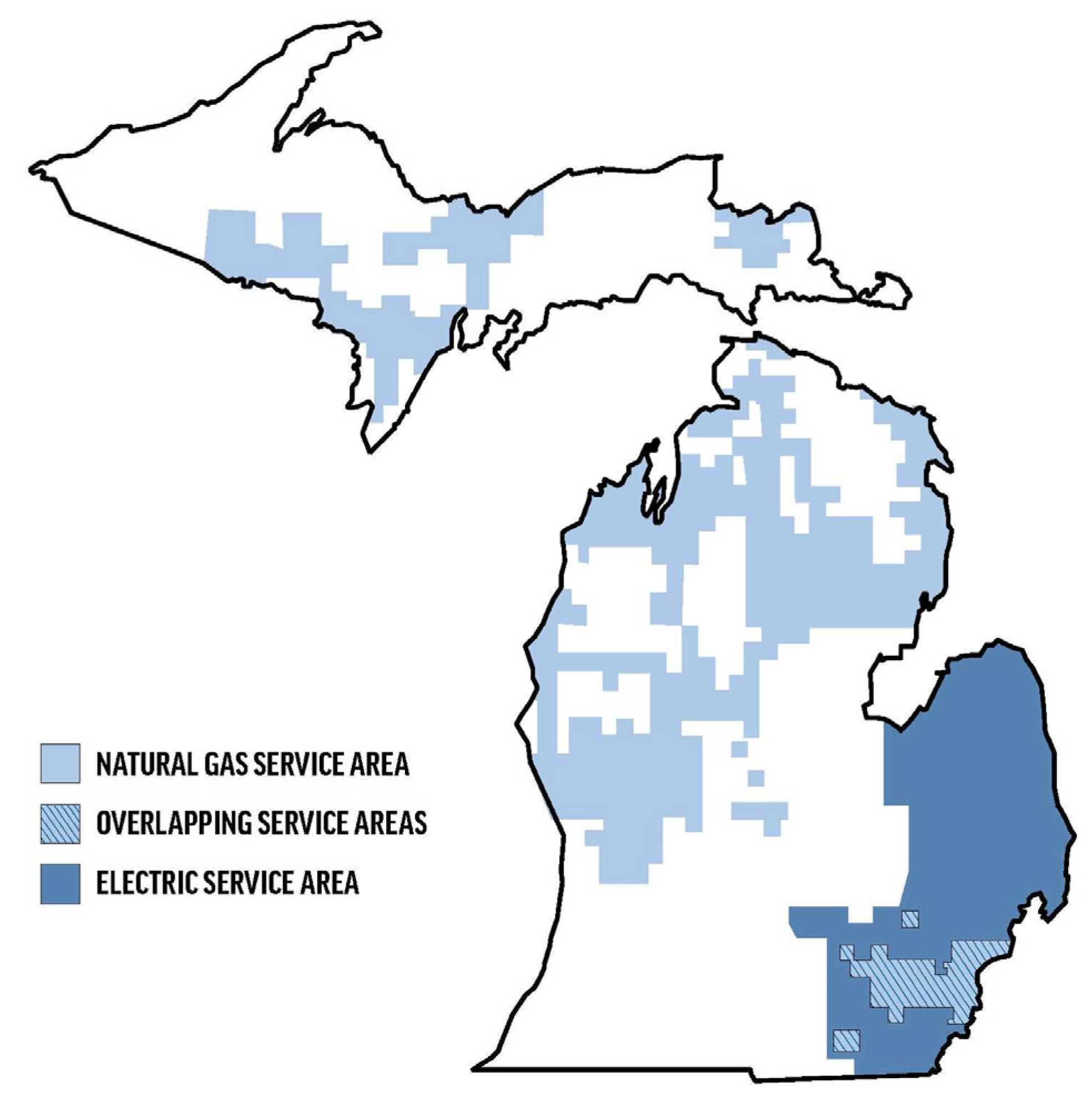
  35. Service Area Map|DTE Energy. Available online: https://aem-qan1.newlook.dteenergy.com/us/en/residential/service-request/moving/service-area-map.html (accessed on 13 October 2023).
  36. Raychaudhuri, S. Introduction to Monte Carlo Simulation. In Proceedings of the 2008 Winter Simulation Conference, Miami, FL, USA, 7–10 December 2008; pp. 91–100. [Google Scholar] [CrossRef]
  37. McClave, J.T.; Benson, P.G.; Sincich, T. Statistics for Business and Economics, 7th ed.; Prentice Hall College Div: Upper Saddle River, NJ, USA, 1998; ISBN 978-0-13-840232-9. [Google Scholar]
  38. Abadi, M.; Agarwal, A.; Barham, P.; Brevdo, E.; Chen, Z.; Citro, C.; Corrado, G.S.; Davis, A.; Dean, J.; Devin, M.; et al. Tensorflow: Large-Scale Machine Learning on Heterogeneous Systems. arXiv 2015, arXiv:1603.04467 2015. [Google Scholar]
  39. Reback, J.; McKinney, W.; Jbrockmendel; Bossche, J.V.D.; Augspurger, T.; Cloud, P.; Gfyoung; Hawkins, S.; Sinhrks; Roeschke, M.; et al. Pandas-Dev/Pandas: Pandas 1.2.2 2021, Version v1.2.2. Available online: https://pandas.pydata.org/ (accessed on 13 October 2023). [CrossRef]
  40. Harris, C.R.; Millman, K.J.; Van Der Walt, S.J.; Gommers, R.; Virtanen, P.; Cournapeau, D.; Wieser, E.; Taylor, J.; Berg, S.; Smith, N.J.; et al. Array Programming with NumPy. Nature 2020, 585, 357–362. [Google Scholar] [CrossRef] [PubMed]
  41. Pedregosa, F.; Varoquaux, G.; Gramfort, A.; Michel, V.; Thirion, B.; Grisel, O.; Blondel, M.; Prettenhofer, P.; Weiss, R.; Dubourg, V.; et al. Scikit-Learn: Machine Learning in Python. J. Mach. Learn. Res. 2011, 12, 2825–2830. [Google Scholar]
  42. RAPIDS Development Team RAPIDS: Libraries for End to End GPU Data Science, Version 23.02. Available online: https://rapids.ai (accessed on 13 October 2023).
  43. Isha, M.T.; Wang, Z. Transformer Hotspot Temperature Calculation Using IEEE Loading Guide. In Proceedings of the 2008 International Conference on Condition Monitoring and Diagnosis, Beijing, China, 21–24 April 2008; pp. 1017–1020. [Google Scholar] [CrossRef]
  44. Wu, Z.; Zhang, J.; Hu, S. Review on Classification Algorithm and Evaluation System of Machine Learning. In Proceedings of the 2020 13th International Conference on Intelligent Computation Technology and Automation (ICICTA), Xi’an, China, 24–25 October 2020; pp. 214–218. [Google Scholar] [CrossRef]
  45. Zhu, N.; Zhu, C.; Zhou, L.; Zhu, Y.; Zhang, X. Optimization of the Random Forest Hyperparameters for Power Industrial Control Systems Intrusion Detection Using an Improved Grid Search Algorithm. Appl. Sci. 2022, 12, 10456. [Google Scholar] [CrossRef]
  46. Sklearn.Svm.SVC. Available online: https://scikit-learn/stable/modules/generated/sklearn.svm.SVC.html (accessed on 13 October 2023).
  47. Sklearn.Ensemble.RandomForestClassifier. Available online: https://scikit-learn/stable/modules/generated/sklearn.ensemble.RandomForestClassifier.html (accessed on 13 October 2023).
  48. Sklearn.Linear_model.LogisticRegression. Available online: https://scikit-learn/stable/modules/generated/sklearn.linear_model.LogisticRegression.html (accessed on 13 October 2023).
  49. Mork, B. Understanding and Dealing with Ferroresonance. In Proceedings of the Minnesota Power Systems Conference, St. Paul, MN, USA, 7–9 November 2006. [Google Scholar]
  50. Iravani, M.R.; Chaudhary, A.K.S.; Giesbrecht, W.J.; Hassan, I.E.; Keri, A.J.F.; Lee, K.C.; Martinez, J.A.; Morched, A.S.; Mork, B.A.; Parniani, M.; et al. Modeling and Analysis Guidelines for Slow Transients. III. The Study of Ferroresonance. IEEE Trans. Power Deliv. 2000, 15, 255–265. [Google Scholar] [CrossRef]
  51. Gokhale, G.S.; Mork, B.A.; O’Donnell, J.; Brehmer, S.R. Ferroresonance Case Study in a Distribution Network and the Potential Impact of DERs and CVR/VVO. Electr. Power Syst. Res. 2023, 220, 109303. [Google Scholar] [CrossRef]
Figure 1. DTE Energy’s Service Territory [35].
Energies 16 07251 g001
Figure 2. An overview of the Monte Carlo structure that is described in this section.
Energies 16 07251 g002
Figure 3. Generating a sequence of day-types for Monte Carlo simulations. (a) An example of day classification with nine clusters, with each cluster represented by a unique index and color. (b) An example Markov chain for January. This work was originally completed with solar irradiance and temperature only, and the dew point was included after the first iterations.
Energies 16 07251 g003
Figure 4. Illustration of the autoregression model used to determine a specific temperature profile for each day in the test period. The arrows illustrate that the earlier hours support forecasting the following hours. The same method is used for solar irradiance and dew point.
Energies 16 07251 g004
Figure 5. Illustration of the outcome of the clustering steps—the Transformer Load Matrix.
Energies 16 07251 g005
Figure 6. Illustration of Neural Network Refinement. The solid line represents the load shape determined from the Load Clustering element of the forecasting method. The Neural Network Refinement element starts with the solid line and refines it to the more accurate dashed line.
Energies 16 07251 g006
Figure 7. Illustration of including standard errors in the Monte Carlo results (a) Standard error table created during the neural network training process; (b) Adding standard errors to the expected value of the forecast. The arrows demonstrate the result of the random selection within the distribution provided by the standard error table, which is illustrated by the dotted lines.
Energies 16 07251 g007
Figure 8. Illustration of Hot-Spot Calculation Determination from IEEE Standard C57.91-2011.
Energies 16 07251 g008
Figure 9. The confusion matrix that was used in this study for predicting power quality events.
Energies 16 07251 g009
Table 1. Transformer parameters used with IEEE Standard C57.91-2011 in this study.
Transformer ParameterHighMidLow
R1074
ΔΘTO,R (°C)605550
τTO (h)864
ΔΘH,R (°C)2517.510
τw (h)0.330.210.083
Table 2. Classification Model Experiment Factors [40,41].
Features Derived from Monte Carlo Simulations Classification MethodHyperparameters
EntropyLogistic Regression (LR)C (SVM and LR)
Percent Greater than 1Support Vector Machine (SVM)Gamma (SVM)
Absolute Difference MeanRandom Forest (RF)Categories Weights (All)
Average Classifier Threshold (All)
Standard Deviation Max Depth (RF)
Maximum Minimum Samples per Leaf (RF)
Minimum
Table 3. The top ten transformers identified as most likely to fail based on Monte Carlo simulations and the IEEE Standard C57.91-2011 Hot-Spot calculations.
Transformer IndexPercent of Monte Carlo
Simulations That Exceeded 100% Useful Life
Transformer Outage EventsData Improvement
Opportunity
Identified
LowMidHigh
2000100100TRUEN/A
38519.2100100FALSETransformer Capacity
4750100100FALSETransformer Capacity
2932.680.7100TRUEN/A
10,3282.725.775TRUEN/A
4890362.7TRUEN/A
2860.12.319.8FALSETransformer Capacity
27502.1100FALSEMeter-to-Transformer Mapping
48001.225.5FALSETransformer Capacity
38900.721.5FALSETransformer Capacity
Table 4. Random Forest Results. The bold line indicates the authors’ preferred option.
Actual Power Quality Event WeightClassifier ThresholdMax DepthMinimum Samples per Leaf Accuracy
× 100
(%)
TPR
× 100
(%)
Precision
× 100
(%)
0.950.52241.2844.1
0.950.52341.2844.1
0.950.53290.1124.7
0.950.53389.8124.5
0.950.42234.3924.0
0.950.42334.3924.0
0.950.43245.0764.0
0.950.43345.6764.1
0.90.52296.0410.0
0.90.52396.2411.1
0.90.53296.6420.0
0.90.53396.8425.0
0.90.42266.1605.2
0.90.42366.1645.5
0.90.43291.62410.5
0.90.43391.72410.7
0.90.44393.3128.1
0.850.43395.949.1
0.90.453395.7813.3
Table 5. Logistic Regression Results.
Actual Power
Quality Event Weight
Classifier ThresholdCAccuracy
× 100
(%)
TPR
× 100
(%)
Precision
× 100
(%)
0.950.51033.9883.9
0.950.5126.2923.6
0.950.50.131.5923.9
0.950.41026.0923.6
0.950.4118.2963.4
0.950.40.113.41003.3
0.90.51067.8686.1
0.90.5166.6605.3
0.90.50.166.7605.3
0.90.41049.1804.5
0.90.4140.1844.1
0.90.40.132.3923.9
Table 6. Feature Ablation Study. This study uses the Random Forest model from Table 4 and removes variables to determine their impact on the results. X indicates the feature is included in the model.
EntropyPercent Greater than 1Abs Diff MeanMax
Load
Min
Load
Average LoadStdev
Load
Accuracy
× 100
(%)
TPR
× 100
(%)
Precision
× 100
(%)
XXXXXXX91.724.010.7
X XXXXX92.024.011.1
X 67.856.05.1
X X 54.676.04.8
XX 72.240.04.4
X XXX 92.912.07.5
XXX 95.18.010.0
XX63.056.04.5
X XXXX94.38.07.4
Disclaimer/Publisher’s Note: The statements, opinions and data contained in all publications are solely those of the individual author(s) and contributor(s) and not of MDPI and/or the editor(s). MDPI and/or the editor(s) disclaim responsibility for any injury to people or property resulting from any ideas, methods, instructions or products referred to in the content.

