Article

Gas–Liquid Flow Behavior in Condensate Gas Wells under Different Development Stages

School of Petroleum Engineering, China University of Petroleum (East China), Qingdao 266580, China
*
Author to whom correspondence should be addressed.
Energies 2023, 16(2), 950; https://doi.org/10.3390/en16020950
Submission received: 13 December 2022 / Revised: 6 January 2023 / Accepted: 12 January 2023 / Published: 14 January 2023
(This article belongs to the Topic Oil, Gas and Water Separation Research)

Abstract

:
The phase state prediction methods of condensate gas are relatively mature, but the effect of phase changes on gas–liquid mixture flow behavior and the liquid-carrying capacity of gas has not been researched in detail. This study applied PIPESIM software to predict the fluid phase properties under different development stages of a condensate gas reservoir in Shengli Oilfield and determined the phase diagram and physical properties of the well stream on the basis of the optimized equation of state (EOS). Then the influence of phase change characteristics on wellbore flow behavior and critical liquid-carrying gas velocity was analyzed. The study showed that compared with the early development stage, fewer heavy components are produced and the produced gas–liquid ratio is increased in the late stage of the condensate gas reservoir. In addition, the pressure loss of fluid is decreased, the critical liquid-carrying gas velocity and flow rate are reduced, and the liquid-lifting difficulty is reduced for gas. The reason is that the liquid density decreases obviously due to the phase change, while the gas density is almost unchanged, and the oil–gas surface tension decreases obviously, resulting in a decrease in the critical liquid-carrying gas velocity. At the same time, the variation in the gas compressibility factor is very small, which leads to a decrease in the critical liquid-carrying gas flow rate.

1. Introduction

The development of a condensate gas reservoir is accompanied by the unique retrograde condensate phenomenon. It is of great significance to clarify the phase change characteristics of condensate gas systems to improve the development effect of condensate gas reservoirs [1]. Researchers have conducted much work on phase state prediction methods. The Soave–Redlich–Kwong (SRK) equation introduces a temperature function to improve the calculation of the effect from actual complex molecular systems such as hydrocarbons on pressure–volume–temperature (PVT) phase characteristics. At present, this method has been widely used in the PVT phase calculation of condensate oil and gas systems [2]. The Peng–Robinson (PR) equation improves the poor accuracy of the SRK equation in predicting a system with strong polar components and the volume characteristics of a liquid, and it can produce satisfactory results when applied to the calculation of gas–liquid two-phase equilibrium physical properties [3,4]. Although numerous EOSs have been reported in the literature, the two-parameter cubic EOSs are still reliable and convenient for estimating lean and rich natural gas properties [5]. The SRK EOS and PR EOS have been proven to be very reliable tools in the prediction of phase behavior and vapor–liquid equilibria [6]. Condensate gas often presents components that have carbon numbers equal to or greater than 7 as plus fractions (C7+) [7]. The heavy ends of condensate gas fluids are considered as having a dominant role in determining the phase behavior, and their molecular weight, density and relative amount have a great influence on the fluid properties [8]. EOS predictions are significantly improved when the C7+ fraction is described by several pseudo-components and an extended higher plus fraction rather than treating it as a single lumped component [9,10], and it is necessary to split the plus fractions into a series of pseudo-components via splitting methods [11]. Thus, accurate prediction of the phase behavior for condensate gas not only relies on the appropriate EOS but also depends on the suitable characterization methods for the plus fraction [12]. In addition, EOS predictions after tuning by regression have become common; this involves the adjustment of groups of EOS parameters so as to minimize the difference between predicted and measured PVT data [13]. Al-Sadoon and Almarry demonstrated the success of tuning by regression for binary interaction coefficients (BICs) between methane and the heavy fractions and the critical pressure, critical temperature and acentric factor for the plus fraction [14].
Several studies have been conducted on the flow behavior in condensate gas wellbores. Juhui Zhu analyzed the dynamic influence of component changes on the wellbore pressure gradient comprehensively in a gas condensate well; he found that condensate liquid dropped out continuously when fluid system pressure was less than dew point pressure, causing the liquid content to increase, and established analytic models to calculate the wellbore pressure profile considering the effect of phase change, but he did not thoroughly study the influence of component changes on parameters such as interfacial tension and the compressibility factor [15]. Adagülü et al. built a model to predict the flowing behavior of gas condensate during production; they combined two-phase flow temperature and pressure profile models and included the effect of composition change for two-phase flow of gas condensate fluid through a wellbore under steady-state conditions. They found that the pressure drop for the varied composition case is higher compared to that of the constant composition case [16]. Yuexin Meng et al. developed a model of wellbore pressure distribution for condensate gas wells; the model was based on gas–liquid equilibrium calculation and combined with wellbore temperature distribution change [17]. Xingguo Liu studied the law of wellbore continuous liquid carrying in a low-permeability gas field; they analyzed the influence of wellhead pressure and temperature on the critical liquid-carrying gas velocity at the wellhead, without considering the influence of fluid component change on liquid-carrying capacity [18]. Zhiping Li et al. proposed a method for calculating the critical flow rate in condensate gas wells with real interfacial tension to improve the accuracy of gas well liquid loading status judgment [19]. The results showed that the accuracy rate of the critical flow rate calculated using the Turner model [20] reached 90%, and this model can be used as the judging standard for the prediction of liquid loading. Chao Zhou et al. optimized methods for liquid loading prediction in deep condensate gas wells. They considered the effect of surface tension along the wellbore in order to improve original critical flow rate models [21].
Literature research and analysis showed that previous studies on phase state calculation have been relatively mature, but the understanding of the changes in wellbore flow behavior and liquid-carrying capacity caused by phase change is not deep enough, and the influence of compositional variation on wellbore flow and liquid-carrying characteristics is less studied.
In this study, the condensate field phase state calculation method was optimized and PIPESIM software was used to accurately predict the phase state of a condensate gas reservoir in the Shengli Oilfield. The changes in fluid physical properties in different development stages were analyzed, and the specific effects of phase changes on wellbore flow behavior and gas-carrying capacity were calculated. The obtained results can provide a basis for the optimization of condensate gas reservoir development.

2. Selection of Equation of State and Wellbore Flow Pressure Drop Calculation Model

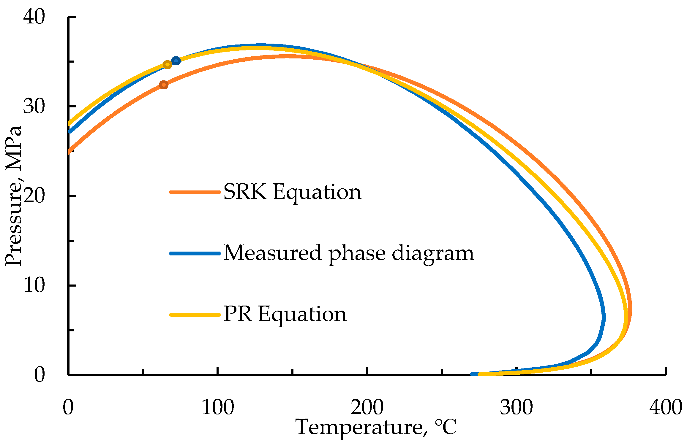
2.1. Optimization of Equation of State

A condensate gas reservoir in Shengli Oilfield was used as a case study. The original pressure of that reservoir is 47.62 MPa, the dew point pressure is 35.2 MPa, the reservoir temperature is 185 °C, the buried depth is 4330 m and the permeability is 2.5 × 10⁻³ um2. It has the characteristics of a small difference between the original reservoir pressure and the dew point pressure, high temperature and low permeability, so the retrograde condensate phenomenon occurs easily in the near-wellbore area. A constant volume depletion (CVD) experiment was by the geological science research institute of Shengli Oilfield performed to simulate reservoir depletion performance and compositional variation. The experimental configurations and procedures followed the oil and gas industry standards of the People’s Republic of China SY/T 5542-2009 Test method for reservoir fluid physical properties. The CVD experiment process was also described by Whitson [22] and Yuan [23] in detail. The experimental data measured in a CVD test include dew point pressure, the composition of the produced gas and the retrograde liquid drop-out curve at different pressure depletion stages. The experimental results of constant volume depletion of this gas reservoir under 185 °C are shown in Table 1.
Firstly, the precision of phase diagram calculation is improved by the optimization of the equation of state. At present, the most commonly used equations of state for condensate gas wells are the PR equation and SRK equation. According to the experimental data of constant volume depletion, the Multiflash package supported in PIPESIM software was used to optimize the two equations of state. The optimization procedure includes C11+ fraction characterization and tuning the EOS parameters according to dew point pressure. The Multiflash package split the C11+ fraction into 6 pseudo-components and determined their molecular weight, specific gravity, critical properties and acentric factor. The comparison results of phase diagram prediction are shown in Figure 1.
Since the range of production temperature in this condensate gas well is 0–185 °C, the phase diagram in the temperature range of 0–200 °C is used for comparison. The mean relative errors of the phase diagrams calculated by the PR equation and SRK equation are 0.98% and 4.46%, respectively. The calculated results of the PR equation of state are closer to the actual phase diagram, so the PR equation was selected for the phase property calculation in the compositional model of PIPESIM software.

2.2. Optimization of Wellbore Flow Pressure Drop Calculation Model

Previous studies have found that Hagedorn–Brown model [24], Gray model [25], Duns–Ros model [26] and Ansari model [27] are more suitable for gas well calculation among the models of multiphase flow pressure drop in a wellbore [28,29,30]. In this study, reservoir test data of the condensate gas well (Table 2) were used to optimize the multiphase flow pressure gradient calculation method.
The bottom-hole flow pressure was selected as the basis point, and the comparative analysis of the calculation errors of six differential pressure measurement points is shown in Table 3; the four models selected have small errors in the calculation of multiphase flow in a condensate gas well in this reservoir, and the calculation error of the Ansari model is at least 8.68%. Therefore, the Ansari model is chosen to calculate the pressure gradient of multiphase flow in the wellbore.

3. Fluid Phase Changes in Different Development Stages of a Condensate Gas Reservoir

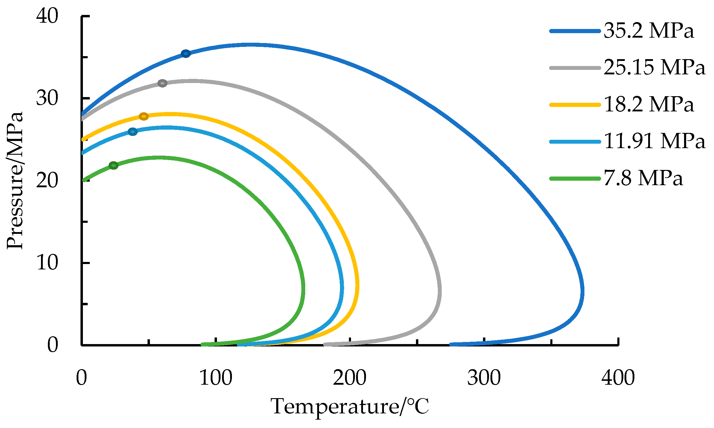
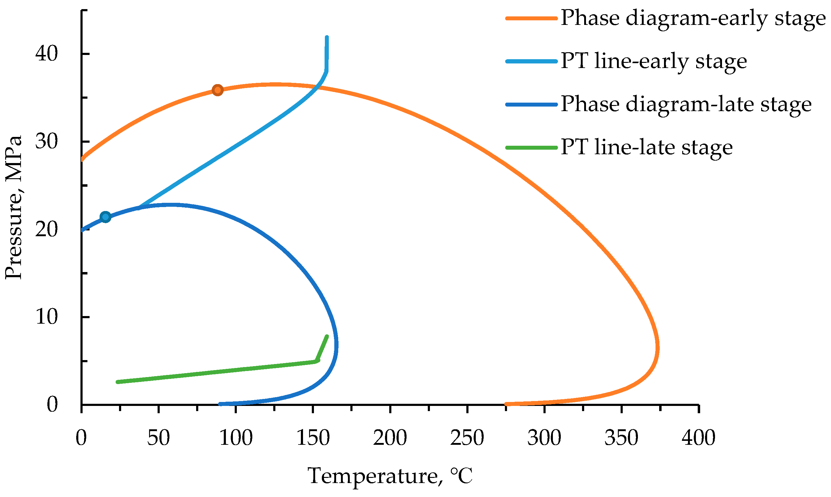
3.1. Phase Diagrams of Produced Fluids in Different Development Stages

The constant volume depletion data of the gas reservoir at 185 °C are shown in Table 1. It can be seen from Table 1 that with the decrease in gas reservoir pressure, the content of light components represented by C1 shows an increasing trend, while the content and molecular weight of heavy components represented by C11+ show a decreasing trend. This indicates that with the decrease in reservoir pressure, heavy components are trapped in the gas reservoir due to the retrograde condensate effect, which changes the composition of the produced fluid, the content of light components represented by C1 increases, while the content of heavy components represented by C11+ decreases and its molecular weight decreases.
The phase diagram obtained by using the optimized phase state calculation method based on the experimental data of constant volume depletion is shown in Figure 2. As shown in Figure 2, in the depletion production process of a condensate gas reservoir, the envelope of the phase diagram will shrink inward, the two-phase flow range will be narrower and the critical point will move to the lower left. This indicates that with the decrease in reservoir pressure, the occurrence of the retrograde condensate phenomenon leads to a change in composition and thus changes the phase diagram.

3.2. The Change in Physical Properties of Produced Fluid in Different Development Stages

In order to study the fluid physical property changes in the bottom hole under different development stages, PIPESIM software was used to calculate the physical properties according to the fluid composition measured by the constant volume depletion; the results are shown in Table 4.
According to the data in Table 4, with the decrease in bottom-hole pressure, some heavy components condense and stay in the formation without participating in the flow. The composition of the flowing fluid changes, while the proportion of light components in the flowing fluid increases, and the molecular weight of the fluid decreases.
In order to study the change in fluid composition and its influence at different stages further, the temperature of 25 °C and pressure of 5 MPa were set to simulate the wellhead conditions, and the change results of the physical properties of each phase of the fluid were calculated and are shown in Table 5.
As can be seen from Table 5, with the decrease in reservoir pressure, some heavy components are precipitated and cannot be carried to the wellhead by gas, resulting in a slight increase in the molecular weight of the gas and a significant decrease in the molecular weight of the oil in the fluid produced at the wellhead. The fluid component involved in the flow becomes lighter, the oil density and viscosity decrease greatly, the gas density and viscosity are almost unchanged, the gas mass fraction increases, the liquid mass fraction decreases, and the produced gas–liquid ratio increases significantly.

4. Gas–Liquid Flow Behavior in a Condensate Gas Well under Different Development Stages

PIPESIM software was used to simulate wellbore flow conditions in different stages of depletion development. The changes in wellbore fluid physical properties in different stages and their effects on pressure gradient and capacity of gas to carry liquid were analyzed.

4.1. Basic Data of Calculation and Analysis

4.1.1. Method for Dividing the Development Stages

When the reservoir pressure is greater than the dew point pressure, the condensate gas flow is single-phase in the formation. When the reservoir pressure is less than the dew point pressure, the condensate oil is precipitated in the formation and the flow is gas–liquid phase in the formation. Considering the relationship between the bottom-hole pressure and the dew point pressure, the development of a condensate gas reservoir can be divided into three stages: the early stage is when the reservoir pressure is greater than the dew point pressure, the middle stage is when the reservoir pressure is slightly less than the dew point pressure, and the late stage occurs when the reservoir pressure is much less than the dew point pressure. In order to compare flow behavior in the wellbore under different stages, the gas production in each stage was set as 2 × 10⁴ sm3/d, and the well productivity data in each period are shown in Table 6.

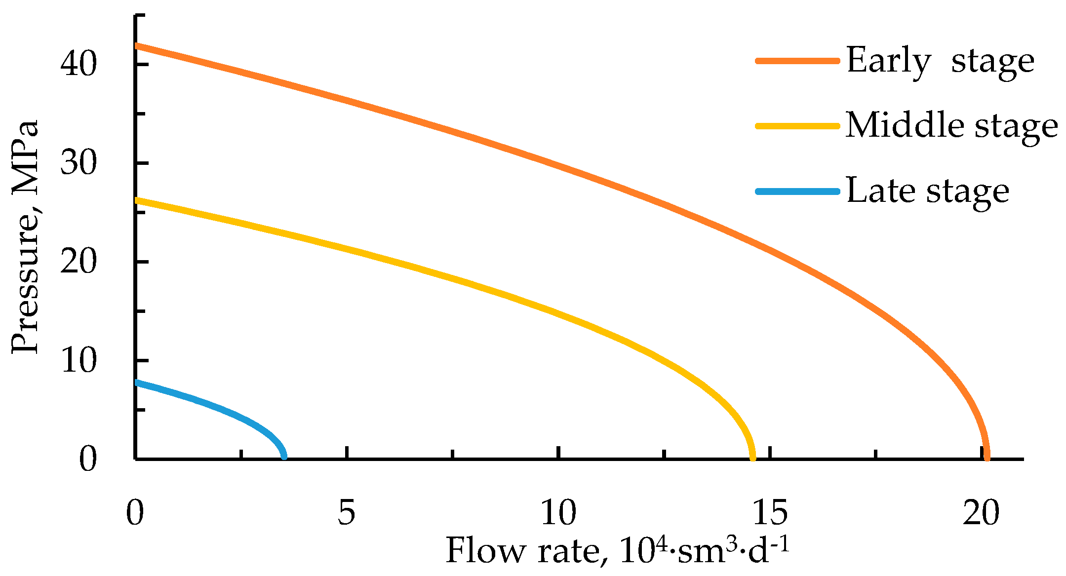
4.1.2. Inflow Performance Relationship (IPR) Curve of a Gas Well

Before fluid flow behavior in the wellbore is analyzed, it is necessary to know the inflow performance relationship curve. In the early stage, the inflow performance relationship curve is established based on gas reservoir test data, and in the middle and late stages, the inflow performance relationship curve is established by numerical simulation, as shown in Figure 3.

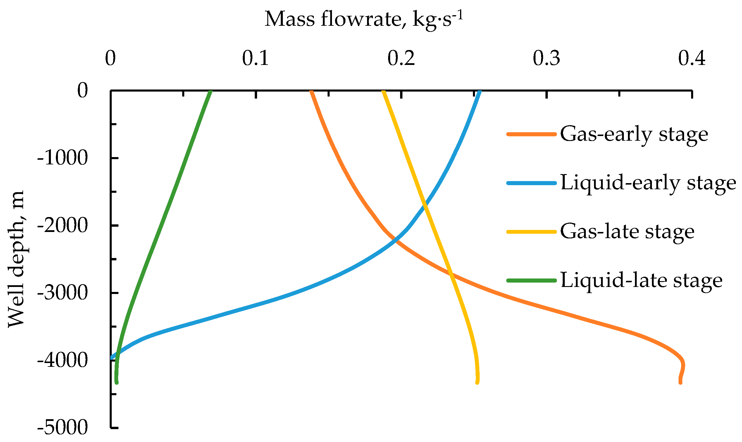
4.2. Analysis of Wellbore Flow Behavior under Different Development Stages

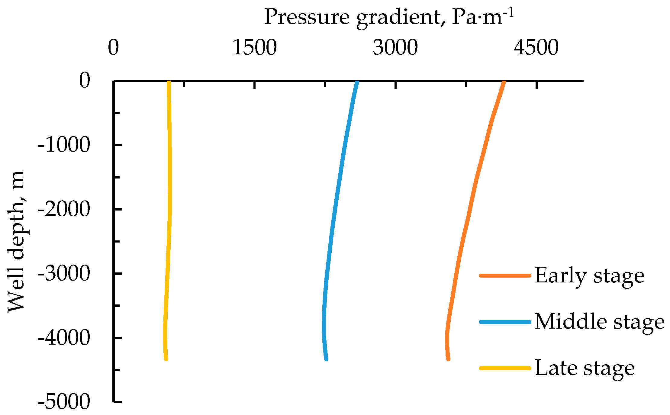
4.2.1. Analysis of Pressure Gradient in a Wellbore

Combined with the PR equation of state optimized above, the gas–liquid ratio was calculated as 1057.42 Sm3/m3 in the early stage of development, 1960.26 Sm3/m3 in the middle stage and 5698.75 Sm3/m3 in the late stage. Therefore, the changes in wellbore pressure drop curves with different gas–liquid ratios were analyzed. The Ansari model was used to calculate the pressure profile of multiphase flow in the wellbore, and the pressure gradient changes in different stages were obtained as shown in Figure 4. The mixture density and gas mass fraction in different development stages are shown in Table 7.
As can be seen from Figure 4, the wellbore pressure gradient decreases significantly with the decrease in reservoir pressure, and the wellbore pressure gradient in the late stage is about 15% of that in the early stage. The main reason is that the wellbore pressure gradient changes due to the changes in gas mass fraction and mixture density in different stages. It can be seen from Table 7 that the variation trend of mixture density is roughly the same as that of the wellbore pressure gradient. As the development progresses, due to the decrease in reservoir pressure, some heavy components condense and stay in the reservoir formation, so the gas mass fraction and the gas–liquid ratio increase in the wellbore. As a result, the mixture density and the wellbore pressure gradient decrease significantly.
It can be also found from Figure 4 that the pressure gradient increases with the decrease in depth along the wellbore in the same development stage, which is exactly the opposite of the situation in the oil well. The reason is that with the decrease in the depth, the crude oil in the oil well keeps releasing gas, and the gas mass fraction keeps increasing, which leads to a decrease in the density of the mixture. However, in the condensate gas well, the condensate oil keeps releasing from the gas along the wellbore, and the increase in the oil mass fraction leads to the increase in the density of the mixture.
In order to understand the retrograde condensate phenomenon in the wellbore further, the calculated phase diagram of produced fluid and the working curves of fluid temperature and pressure were plotted, as shown in Figure 5. The gas mass flow rate and liquid mass flow rate are shown in Figure 6. Because the variation rules are similar between the middle and late stages, only the curves of parameters in the early stage and late stage are shown in Figure 6 for the sake of conciseness and clarity.
It can be seen from Figure 5 that condensate oil did not precipitate in the formation and the retrograde condensate phenomenon only appeared in the wellbore in the early development stage. In the late stage, the phase diagram gradually shrank, the critical point moved downward, the critical condensate pressure and the critical condensate temperature decreased, and condensate oil began to precipitate in the formation.
In the early stage, the mass flow rate of gas first remained constant and then decreased with the decrease in depth. As shown in Figure 6, condensate oil began to precipitate at the depth of 3962.4 m, and the amount of oil precipitated gradually increased along the wellbore. However, in the later stage, condensate oil appeared at the bottom of the well. In the process of condensate gas production, the quality of gas in the wellbore is transferred to the liquid, and only the condensate phenomenon occurs in the wellbore, without the condensate oil evaporation phenomenon.

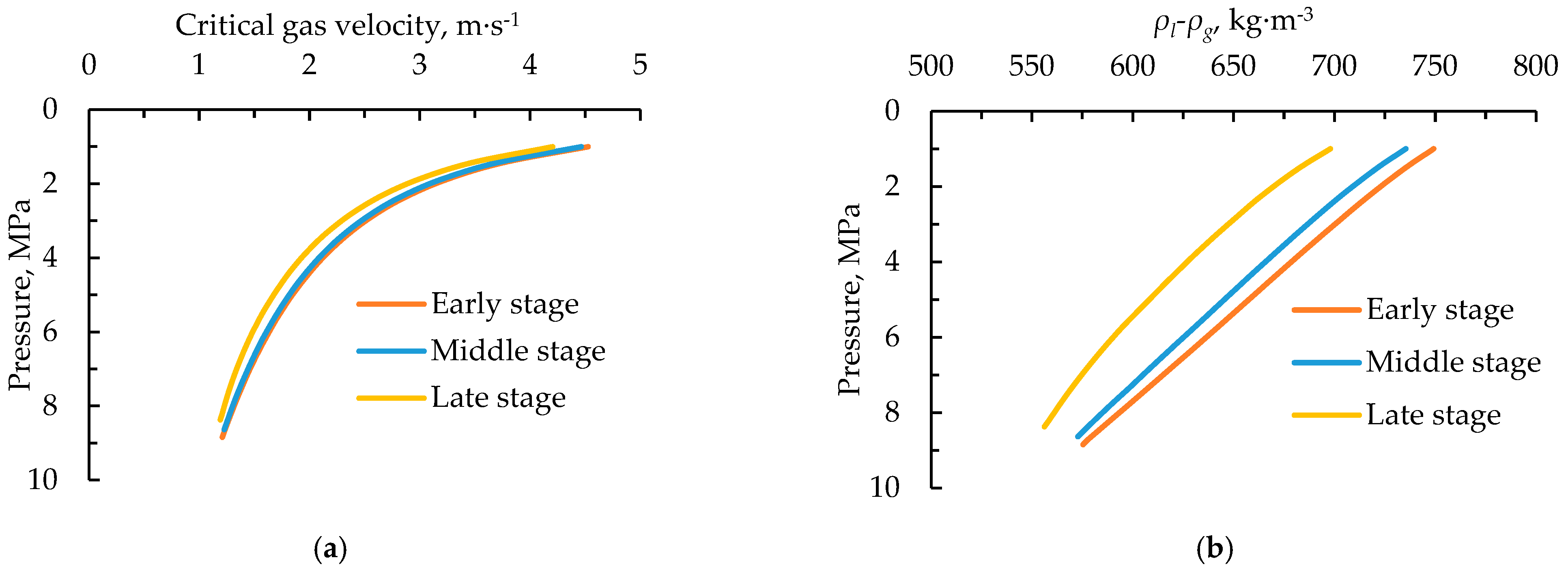
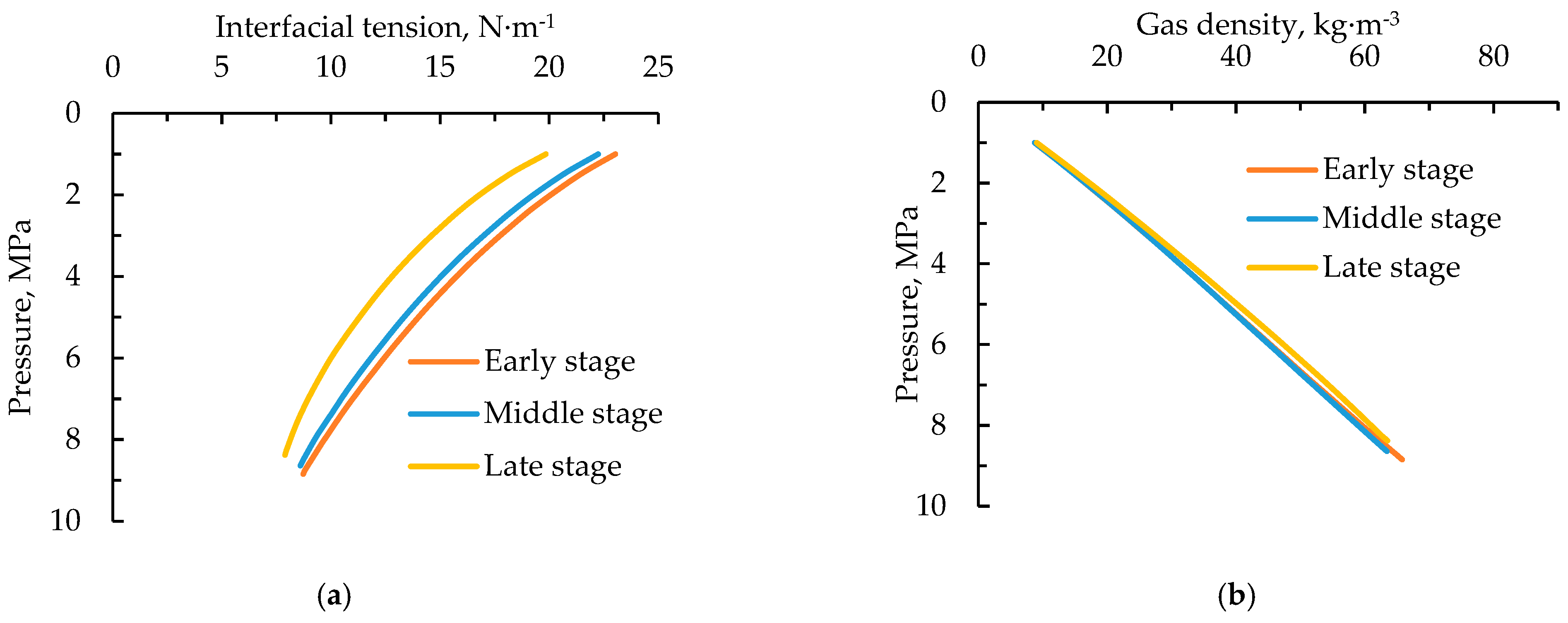
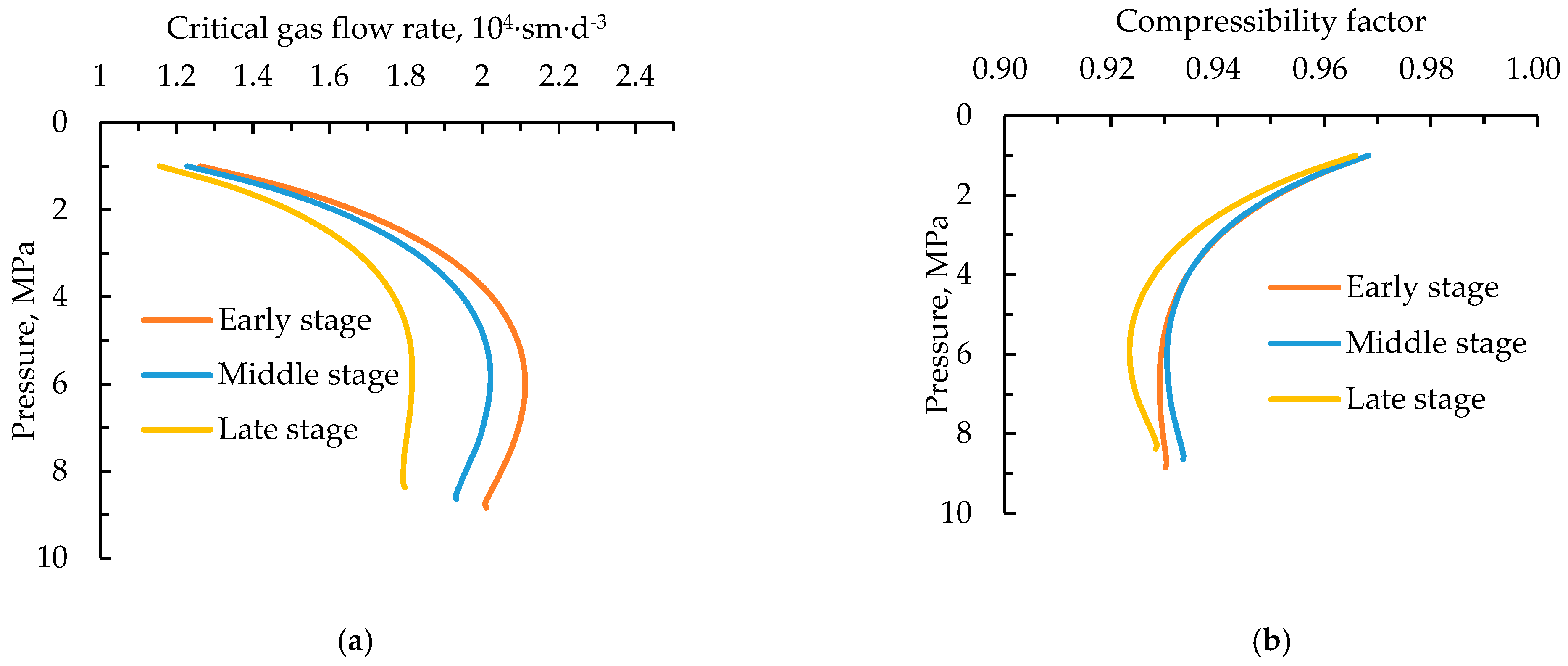
4.2.2. Analysis of Critical Liquid-Carrying Gas Velocity

Calculation Formula of Critical Liquid-Carrying Gas Velocity

In the early stage of gas reservoir development, natural gas can be continuously produced from the wellbore. At this time, the liquid in the wellbore exists in the form of small droplets, and the gas is in a continuous phase. With the continuous development of natural gas, the natural gas production rate decreases, gas velocity in the wellbore decreases and condensate oil is produced continuously. If the gas velocity is insufficient to carry out all the droplets, liquid accumulation will eventually be formed at the bottom of the well. The minimum gas velocity required to bring the largest possible droplet to the surface in this process is called the critical velocity [31]. The Turner model in PIPESIM software is widely used in the calculation of liquid carrying in various gas reservoirs [20]. Its expression is shown in Equation (1):
v t = 6.6 [ σ ( ρ l ρ g ) ] 0.25 ρ g 0.5
where vt is the critical liquid-carrying gas velocity, m/s; ρg is gas density, kg/m3; ρl is the liquid density, kg/m3; and σ is surface tension, N/m.
The critical liquid-carrying gas flow rate is the minimum flow rate at which the liquid can be carried, and its calculation formula is shown in Equation (2). It can be seen from the formula that the factors affecting the critical flow rate are the tubing cross-section area, critical gas velocity, pressure, temperature and compressibility factor.
q = 2.5 × 10 4 A v t p Z T
where q is the critical liquid-carrying gas flow rate, 104 sm/d3; A is the section area of tubing, m2; vt is the critical gas velocity, m/s; p is pressure, MPa; Z is the compressibility factor; and T is the temperature, K.

Effect of Fluid Component Change on Liquid-Carrying Capacity

In the process of fluid flow from the bottom hole to the wellhead, the liquid-carrying capacity of gas is affected by fluid composition, pressure and temperature. The influence of component change on liquid-carrying velocity is actually caused by interfacial tension, liquid–gas density difference and gas density change. In order to study the influence of component changes on the liquid-carrying capacity of gas in different development stages, the changes in various physical parameters were calculated from the wellhead to the bottom hole under the condition that the wellhead pressure was 1 MPa and the gas production was 1 × 10⁴ m3/d. The critical liquid-carrying gas velocity in different stages was calculated as shown in Figure 7a.
As can be seen from Figure 7a, the critical gas velocity increases significantly with the decrease in pressure during the same development stage, and the maximum critical gas velocity is reached at the wellhead. Under the same pressure condition in the wellbore in different development stages, the critical liquid-carrying gas velocity required in the later stage is smaller.
According to the Turner formula, the critical liquid-carrying velocity is related to interfacial tension, gas density, and the density difference between liquid and gas. In order to study the influence of component changes on the critical gas velocity further, PIPESIM software was used to determine the density difference between liquid and gas, interfacial tension and gas density along the wellbore in different development stages, as shown in Figure 7b and Figure 8a,b.
It can be seen that the physical properties of the three development stages have the same trend of variation with depth. Taking the late stage as an example, as the wellbore depth decreases, the pressure and temperature decrease, the gas density decreases significantly, the density difference between liquid and gas increases significantly, and the physical difference between gas and liquid becomes greater, resulting in a significant increase in interfacial tension, so the critical gas velocity will increase greatly and reach the maximum value at the wellhead. The critical gas velocity at the wellhead is about 3.5 times that at the bottom hole, and the amplitude of the increase is very obvious.
Under the same pressure and temperature conditions, the critical gas velocity in the late stage of development is slightly lower than that in the early and middle stages. The reason is that, with the continuous depletion development of the condensate reservoir, the retrograde condensate phenomenon leads to the retention of more components in the reservoir, thus reducing the density of the liquid and the surface tension of the liquid, while the density of the gas does not change much. Therefore, the critical gas velocity gradually decreases with the development time.
Equation (2) shows that the influence of component changes on critical liquid-carrying gas flow rate is actually the influence of critical gas velocity and compressibility factor changes under the same flow conditions. PIPESIM software was used to calculate the critical gas flow rate along the wellbore, as shown in Figure 9a. As can be seen from the figure, under the same pressure and temperature conditions, the critical gas flow rate in the middle and late stages of development is smaller than that in the early stage. In the same stage, with the decrease in depth and pressure, the critical gas flow rate increases slightly first and then decreases obviously.
In order to study the reasons for the change in critical gas flow rate further, the change in gas compressibility factor was calculated, as shown in Figure 9b. It can be seen from Figure 7a and Figure 9a,b that the critical gas flow rate, critical gas velocity and compressibility factor in different development stages have roughly the same variation trend. The compressibility factor at the same pressure in different stages is less affected by the change in components, and the critical gas velocity decreases in the middle and late stages of development, so the flow rate required to carry liquid decreases in the middle and late stages, and it is easier for gas to carry liquid than in the early stages.
In the same development stage, taking the late development stage as an example, as the depth decreases, the pressure decreases, and the compressibility factor decreases slightly first and then increases, while the critical gas velocity increases along the depth of the well, so the critical flow rate increases slightly first and then decreases with the decrease in depth decreasing. The critical gas flow rate at the bottom of the well is about 1.5 times that at the wellhead.

5. Conclusions

(1) Through the calculation and analysis of the constant volume depletion experiment data, it can be seen that with the continuous production of a condensate reservoir in the depletion development process, the produced fluid phase diagram shrinks continuously, the two-phase region narrows, and the critical point moves to the lower left as the reservoir pressure drops. The fraction of light components in produced fluid increased, the fraction of heavy components decreased, the condensate oil density at the wellhead became lighter, both the condensate gas density and molecular weight were almost unchanged, and the production gas–liquid ratio increased significantly.
(2) Compared with the early stage, the mass fraction of gas in produced fluid increases in the late stage of development, which greatly reduced the density and pressure gradient of the mixture. During the same development stage, only the retrograde condensate phenomenon occurred with the decrease in depth during the production of well fluid, but no condensate oil evaporation phenomenon occurred. As a result, the mass fraction of the liquid increased continuously, and the mixture density and pressure gradient increased continuously.
(3) Compared with the early stage of development, due to the change in components, the density difference between the gas and liquid and the interfacial tension decrease, and the density of the gas is almost unchanged, so both critical liquid-carrying gas velocity and critical liquid-carrying gas flow rate decrease under the same pressure and temperature conditions. That is, liquid carrying is easier in the late stage of development. During the same development period, with the comprehensive influence of critical gas velocity and compressibility factor, the critical gas flow rate increases slightly first and then decreases obviously with the decrease in well depth.

Author Contributions

Formal analysis, M.L.; investigation, W.Z.; methodology, W.W.; supervision, M.L.; writing—original draft, W.Z.; writing—review and editing, W.W. All authors have read and agreed to the published version of the manuscript.

Funding

This research was funded by the National Natural Science Foundation of China, grant number 52174056.

Data Availability Statement

All the data are included in this paper.

Conflicts of Interest

The authors declare no conflict of interest.

References

  1. Liu, H.; Sun, C.-Y.; Yan, K.-L.; Ma, Q.-L.; Wang, J.; Chen, G.-J.; Xiao, X.-J.; Wang, H.-Y.; Zheng, X.-T.; Li, S. Phase behavior and compressibility factor of two China gas condensate samples at pressures up to 95 MPa. Fluid Phase Equilibria 2013, 337, 363–369. [Google Scholar] [CrossRef]
  2. Soave, G. Equilibrium constants from a modified Redlich-Kwong equation of state. Chem. Eng. Sci. 1972, 27, 1197–1203. [Google Scholar] [CrossRef]
  3. Peng, D.-Y.; Robinson, D.B. A new two-constant equation of state. Ind. Eng. Chem. Fundam. 1976, 15, 59–64. [Google Scholar] [CrossRef]
  4. Li, S.L. Natural Gas Engineering, 2rd ed; Petroleum Industry Press: Beijing, China, 2008; pp. 63–65. [Google Scholar]
  5. Nasrifar, K.; Bolland, O. Prediction of thermodynamic properties of natural gas mixtures using 10 equations of state including a new cubic two-constant equation of state. J. Pet. Sci. Eng. 2006, 51, 253–266. [Google Scholar] [CrossRef]
  6. Nazarzadeh, M.; Moshfeghian, M. New volume translated PR equation of state for pure compounds and gas condensate systems. Fluid Phase Equilibria 2013, 337, 214–223. [Google Scholar] [CrossRef]
  7. Bonyadi, M.; Esmaeilzadeh, F. Prediction of gas condensate properties by Esmaeilzadeh-Roshanfekr equation of state. Fluid Phase Equilibria 2007, 260, 326–334. [Google Scholar] [CrossRef]
  8. Elsharkawy, A.M. Predicting the dew point pressure for gas condensate reservoirs: Empirical models and equations of state. Fluid Phase Equilibria 2002, 193, 147–165. [Google Scholar] [CrossRef]
  9. Al-Meshari, A.A.; McCain, W.D. Validation of splitting the hydrocarbon plus fraction: First step in tuning equation-of-state. In Proceedings of the SPE Middle East Oil and Gas Show and Conference, Bahrain, Bahrain, 11–14 March 2007. [Google Scholar]
  10. Dandekar, A.Y. Effect of Fluid Characterization on CVD Liquid Drop-out Predictions of Gas Condensate Fluids Using an Equations of State Model. Energy Sources Part A 2008, 30, 1548–1562. [Google Scholar] [CrossRef]
  11. Whitson, C.H. Characterizing hydrocarbon plus fractions. SPE J. 1983, 23, 683–694. [Google Scholar] [CrossRef]
  12. Nasrifar, K.; Bolland, O.; Moshfeghian, M. Predicting natural gas dew points from 15 equations of state. Energy Fuels 2005, 19, 561–572. [Google Scholar] [CrossRef]
  13. Agarwal, R.K.; Li, Y.K.; Nghiem, L. A regression technique with dynamic parameter selection for phase-behavior matching. SPE Res. Eng. 1990, 5, 115–119. [Google Scholar] [CrossRef]
  14. Almarry, J.A.; Al-Sadoon, F.T. Prediction of liquid hydrocarbon recovery from a gas condensate reservoir. In Proceedings of the Middle East Oil Technical Conference and Exhibition, Bahrain, Bahrain, 11–14 March 1985. [Google Scholar]
  15. Zhu, J.H.; Hu, Y.Q.; Zhao, J.Z.; Zhang, R.Z. Calculation on change in borehole pressure of gas condensate well at the condition of phase change. Pet. Geol. Oilfield Dev. Daqing 2006, 26, 50–52. [Google Scholar]
  16. Adagülü, D.; Gumrah, F.; Sinayuç, C. Wellbore Modeling for Predicting the Flowing Behavior of Gas Condensate during Production. Energy Sources Part A 2009, 31, 783–795. [Google Scholar] [CrossRef]
  17. Meng, Y.X.; Li, X.F.; Yin, B.T.; Qi, M.M. The calculation of wellbore pressure distribution for condensate wells. J. Eng. Therm. 2010, 31, 1508–1512. [Google Scholar]
  18. Liu, X.G.; Yue, J.W.; Yi, F. Study on Law of Wellbore Continuous Liquid Carrying in Low Permeability Gas Field. Sino-Global Energy 2012, 17, 65–67. [Google Scholar]
  19. Li, Z.P.; Guo, Z.Z.; Lin, N. Calculation Method of Critical Flow Rate in Condensate Gas Wells Considering Real Interfacial Tension. Sci. Techol. Rev. 2014, 32, 28–32. [Google Scholar]
  20. Turner, R.G.; Hubbard, M.G.; Dulker, A.E. Analysis and prediction of minimum flow rate for the continuous removal of liquids from gas wells. J. Pet. Techol. 1969, 21, 1475–1482. [Google Scholar] [CrossRef]
  21. Zhou, C.; Wu, X.; Li, H.; Lin, H.; Liu, X.; Cao, M. Optimization of methods for liquid loading prediction in deep condensate gas wells. J. Pet. Sci. Eng. 2016, 146, 71–80. [Google Scholar] [CrossRef]
  22. Whitson, C.H.; Torp, S.B. Evaluating Constant-Volume Depletion Data. J. Pet. Techol. 1983, 35, 610–620. [Google Scholar] [CrossRef]
  23. Yuan, S.Y. Theory and Practice of Efficient Development of Condensate Gas Reservoirs, 1st ed.; Petroleum Industry Press: Beijing, China, 2003; pp. 8–11. [Google Scholar]
  24. Hagedorn, A.R.; Brown, K.E. Experimental study of pressure gradients occurring during continuous two-phase flow in small-diameter vertical conduits. J. Pet. Techol. 1965, 17, 475–484. [Google Scholar] [CrossRef]
  25. Brill, J.P.; Mukherjee, H. Multiphase Flow in Wells; Society of Petroleum Engineers of AIME: Richardson, TX, USA, 1999; pp. 31–32. [Google Scholar]
  26. Duns, H., Jr.; Ros, N.C.J. Vertical flow of gas and liquid mixtures in wells. In Proceedings of the Sixth World Petroleum Congress, Frankfurt, Germany, 19–26 June 1963. [Google Scholar]
  27. Ansari, A.M.; Sylvester, N.D.; Sarica, C.; Shoham, O.; Brill, J.P. A comprehensive mechanistic model for upward two-phase flow inwellbores. SPE Prod. Facil. 1994, 9, 143–152. [Google Scholar] [CrossRef] [Green Version]
  28. Liao, K.G.; Li, Y.C.; Yang, Z.; Zhong, H.Q. Study on pressure drop models of gas-liquid two-phase pipe flow in gas reservoir. Acta Petrolei Sin. 2009, 30, 607–612. [Google Scholar]
  29. Tian, Y.; Wang, Z.B.; Li, Y.C.; Bai, H.F.; Li, K.Z. Evaluation and optimization of wellbore pressure drop model for drainage and gas recovery by velocity string. Fault-Block Oil Gas Field 2015, 22, 130–133. [Google Scholar]
  30. Chen, D.C.; Xu, Y.X.; Meng, H.X.; Peng, G.Q.; Zhou, Z.F. Evaluation and optimization of pressure drop calculation models for gas-liquid two-phase pipe flow in gas well. Fault-Block Oil Gas Field 2017, 24, 840–843. [Google Scholar]
  31. Lea, J.F.; Nickens, H.V.; Wells, M.R. Gas Well Deliquification, 2nd ed.; Elsevier Press: Amsterdam, The Netherlands, 2003; pp. 31–34. [Google Scholar]
Figure 1. Comparison of predicted phase diagrams of PR EOS and SRK EOS.
Energies 16 00950 g001
Figure 2. Fitting phase diagram of constant volume depletion.
Energies 16 00950 g002
Figure 3. Inflow performance relationship curves for different periods.
Energies 16 00950 g003
Figure 4. Pressure gradient changes along the wellbore at different stages.
Energies 16 00950 g004
Figure 5. The well fluid phase diagram, fluid PT lines in different periods.
Energies 16 00950 g005
Figure 6. The mass flow rate in different periods.
Energies 16 00950 g006
Figure 7. (a) The change in critical gas velocity in different periods; (b) the change in liquid–gas density in different periods.
Energies 16 00950 g007
Figure 8. (a) The change in interfacial tension in different periods; (b) the change in gas density in different periods.
Energies 16 00950 g008
Figure 9. (a) The change in critical gas flow rate in different periods; (b) the change in compressibility factor in different periods.
Energies 16 00950 g009
Table 1. Experimental data of constant volume depletion (mole fraction of different components).
ComponentSymbolPressure, MPa
35.225.1518.211.917.8
Carbon dioxideCO20.01510.01580.01630.01740.0155
MethaneC10.71990.76430.78070.78350.7810
EthaneC20.05170.05310.05380.05500.0559
PropaneC30.03870.03850.04250.04080.0447
iso-ButaneiC40.01100.01060.01170.01120.0124
n-ButanenC40.01980.01850.02030.01970.0218
iso-PentaneiC50.01220.01070.01160.01150.0126
n-PentanenC50.01030.00870.00930.00940.0102
HexanesC60.02170.01620.01390.01460.0147
HeptanesC70.01630.01150.00870.00970.0096
OctanesC80.02000.01370.00850.00840.0075
NonanesC90.01630.01160.00730.00640.0056
DecanesC100.01130.00790.00510.00450.0037
Undecanes PlusC11+0.03560.01890.01010.00780.0048
C11+ Molecular weight217.36200.82192.38190.05178.20
C11+ specific gravity0.85560.84390.83720.83530.8250
Table 2. Reservoir test data of a condensate gas well in Shengli Oilfield.
Choke
Size
Daily Gas Production Rate, m3Daily Oil
Production Rate, tons
Daily Water Production Rate, tonsWellhead
Pressure, MPa
Bottom-Hole Flow
Pressure, MPa
Depth of
Apparatus
Entry, m
Test Pressure, MPa
4 mm34,94932.4021.336.92280031.41
6 mm80,03651.57.2216.433.60280028.09
8 mm118,33681.711.4514.627.21280023.16
Table 3. Calculation error of six pressure measurement points of four multiphase flow calculation methods.
Choke
Size
Choke (4 mm)Choke (6 mm)Choke (8 mm)Error Mean, %
Measurement Point Pressure Error, %Wellhead Pressure
Error, %
Measurement Point Pressure Error, %Wellhead Pressure Error, %Measurement Point Pressure Error, %Wellhead Pressure Error, %
Ansari6.313.559.5313.5311.697.448.68
Gray8.182.8110.5516.6511.148.389.62
Duns–Ros8.649.245.5012.319.676.868.70
Hagedorn–Brown8.163.3110.1416.7010.628.009.49
Table 4. Molecular weight of produced fluid in the bottom hole in the gas reservoir.
Bottom-Hole
Pressure, MPa
35.225.1518.211.917.8
Molecular weight35.5829.4526.4625.9625.42
Table 5. Physical parameters of wellhead produced fluid in the gas reservoir.
Bottom-Hole
Pressure, MPa
Molecular
Weight
Density, kg m−3Viscosity, mPa sMass
Fraction, %
GasOilGasOilGasOilGasOil
35.219.0788.3244.74689.560.011640.521541.358.7
25.1519.1580.6345.43668.580.011640.424653.146.9
18.219.6173.9146.46646.710.011620.339562.437.6
11.9119.6469.3246.92636.570.011630.310265.234.8
7.819.8265.8147.46614.690.011610.253067.832.2
Table 6. Well productivity data.
Development
Stage
Reservoir Pressure, MPaBottom-Hole
Pressure, MPa
Wellhead
Pressure, MPa
Gas Production Rate, sm3·d−1
Early41.939.722.42 × 104
Middle26.324.314.52 × 104
Late7.85.12.762 × 104
Table 7. The changes in physical properties, gas content and pressure gradient at different stages.
Depth, mMixture Density, kg·m−3Gas Mass Fraction, %Pressure Gradient, Pa·m−1
Early StageMiddle StageLate StageEarly StageMiddle StageLate StageEarly StageMiddle StageLate Stage
−4329345.72 215.71 38.09100.0085.2497.863398 2221 558
−4267345.31 214.81 37.62100.0085.1197.623394 2214 552
−3962345.16 212.66 36.95100.0083.7597.313393 2199 547
−3657347.30 212.75 36.1389.7680.3596.743414 2207 551
−3352350.67 213.94 35.9678.7577.3596.633446 2225 560
−3048354.98 215.40 35.7265.3573.5796.353489 2247 569
−2743359.64 217.14 35.3458.6471.6794.433535 2271 578
−2438362.89 219.07 34.9250.2468.6493.213570 2298 585
−2133366.63 221.41 34.6147.9166.6191.933614 2328 594
−1828370.94 223.54 34.2544.8663.8090.163659 2356 596
−1524376.11 225.94 33.5642.6961.3588.643711 2386 596
−1219380.50 228.63 33.1340.2859.6686.923757 2418 595
−914385.64 231.48 32.5038.9556.3485.363809 2452 594
−609.6391.70 234.44 31.6936.5454.3783.103871 2486 593
−304.8397.78 238.04 31.3435.1653.9281.263932 2527 590
0404.23 241.58 30.3134.2951.9678.433996 2565 584
Disclaimer/Publisher’s Note: The statements, opinions and data contained in all publications are solely those of the individual author(s) and contributor(s) and not of MDPI and/or the editor(s). MDPI and/or the editor(s) disclaim responsibility for any injury to people or property resulting from any ideas, methods, instructions or products referred to in the content.

