Wind Farm Power Prediction Considering Layout and Wake Effect: Case Study of Saudi Arabia

Abstract

The world’s technological and economic advancements have led to a sharp increase in the demand for electrical energy. Saudi Arabia is experiencing rapid economic and demographic growth, which is resulting in higher energy needs. The limits of fossil fuel reserves and their disruption to the environment have motivated the pursuit of alternative energy options such as wind energy. In order to regulate the power system to maintain safe and dependable operation, projections of current and daily power generation are crucial. Thus, this work focuses on wind power prediction and the statistical analysis of wind characteristics using wind data from a meteorological station in Makkah, Saudi Arabia. The data were collected over four years from January 2015 to July 2018. More than twelve thousand data points were collected and analyzed. Layout and wake effect studies were carried out. Furthermore, the near wake length downstream from the rotor disc between 1 and 5 rotor diameters (1D to 5D) was taken into account. Five robust machine learning algorithms were implemented to estimate the potential wind power production from a wind farm in Makkah, Saudi Arabia. The relationship between the wind speed and power produced for each season was carefully studied. Due to the variability in the wind speeds, the power production fluctuated much more in the winter. The higher the wind speed, the more significant the difference in energy production between the five farm layouts, and vice versa, whereas at a low wind speed, there was no significant difference in the power production in all of the near wake lengths of the 1D to 5D rotor diameters downstream from the rotor disc. Among the utilized prediction models, the decision tree regression was found to have the best accuracy values in all four utilized evaluation metrics, with 0.994 in R-squared, 0.025 in MAE, 0.273 in MSE, and 0.522 in RMSE. The obtained results were satisfactory and provide support for the construction of several wind farms, producing hundreds of megawatts, in Saudi Arabia, particularly in the Makkah Region.

1. Introduction

The demand for electrical energy has risen dramatically due to the fact of global technical and economic advances. Rapid population and economic growth in Saudi Arabia is accompanied by increased energy consumption, whether in terms of fuel, electricity, or for desalination.

Saudi Arabia has long relied on coal, petroleum, natural gas, and other fossil resources to generate electricity. For various reasons, there has been an increase in interest in developing new sources of electric power generation in recent years. The most important reason is reducing environmental pollution and anthropogenic greenhouse gas emissions caused by fossil fuel combustion. Finding fossil fuel sources requires great financial investment. This cost is projected to rise in the coming years; the Earth’s supply of fossil fuels is finite, and these resources will become increasingly challenging to locate and maintain indefinitely. On the other hand, wind energy is derived from sources that are regenerated by nature constantly. It is clean, emission free, and environmentally friendly energy, as its production does not cause environmental pollution. In general, there are several reasons to choose wind power, including aiding the environment, securing long-term price stability, securing lower-cost electricity, and reducing the community’s reliance on fossil fuels. With the expansion of scientific advancement and the commercial growth of the wind power sector, human wind power usage has evolved from theoretical experiments to practical production. Wind power’s manufacturing profitability and usefulness are continuously being promoted. An economic study of power systems requires knowledge of a power system’s current and predicted future conditions. Current power production and daily power production predictions are critical in regulating the power system to maintain safe and reliable operation. This impact has an effect on day-ahead unit commitment costs, power system operation costs, and energy market clearing prices. The main contributions of this work can be summarized as follows:

• Investigate the wind characteristics that have a significant impact on wind power production;
• Compare the performance of various machine learning algorithms on predicting the power output of wind farms;
• Evaluate the proposed prediction models utilizing effort estimation assessment metrics;
• Factoring wind farm turbine layout and wake effects in predicting wind power output.

The remainder of this paper is structured as follows. Section 2 discusses electricity consumption. Section 3 highlights the wind energy share and literature review on wind power prediction. The forecasting models and evaluation metrics utilized in this work are introduced in Section 4. Section 5 presents the methodology to predict wind farm power, including the layout and wake effect. The experimental results and discussion are presented in Section 6. Finally, the conclusions are drawn in Section 7.

2. Electricity Consumption and Renewable Energy

For several years fossil fuel energy sources have been used as a based energy resource. However, populations and demands for resources have continuously increased. Alternative energy sources, such as solar, wind, hydropower, geothermal, biomass, and hydrogen, have become more popular as a result of the depletion of fossil fuel supplies and the environmental disruption they cause [1].

Wind power has increased rapidly in recent years as an essential part of renewable energy. Wind energy is produced from the movement of wind, converting kinetic energy into electrical energy through wind turbines (the principle of energy transformation). Determining the location of a wind farm depends mainly on studying the activity of wind movement in the region, which is measured by geographic studies, satellites, and sensor monitoring and measuring devices [2]. Saudi Arabia has taken serious steps in using renewable energy sources, in addition to oil and gas, conserving current resources, achieving balance, ensuring that future generations have the resources they need to live well and attaining economic development. There are several reasons for choosing Makkah as the location for this wind farm case study. It is distinguished by a significant advantage over other cities in Saudi Arabia, which is the presence of the Noble Sanctuary, which requires operation 24 h a day, year round. Moreover, millions of people flock to Makkah during the Hajj and Umrah seasons and, thus, the demand for electricity in this city is higher than in other cities.

In the following subsections, detailed statistics regarding electricity consumptions are provided. Further, the capacity of renewable energy and the status of wind energy in Saudi Arabia are highlighted.

2.1. Electricity Consumption in Saudi Arabia

Saudi Arabia has one of the highest global rates of electricity use per capita. In addition, this consumption rate rose from 6.9 to 9.6 MWh during the period between 2007 and 2017. Furthermore, Saudi Arabia’s share of residential electricity usage accounts for the largest share of overall electricity consumption, which, in 2017, increased by approximately 48% [3].

2.1.1. Electricity Consumption in Saudi Arabia

The total electricity consumption in Saudi Arabia in 2018, according to the Electricity and Cogeneration Regulatory Authority (ECRA), was 299,188 GWh, with 101,159 GWh of this being in the western region. The electrical energy consumption in residential sectors was 130,428 GWh [4].

2.1.2. Daily Average of Saudi Household Consumption

Household power consumption is the energy consumed by the population for domestic purposes only (water heating, warming, air-conditioning, lighting, cooking, etc.). A survey sample was taken consisting of 22,000 households distributed by administrative regions across Saudi Arabia, and 3900 were in the Makkah Region. The percentage of dwellings using public electricity throughout Saudi Arabia was 99.5%. The rate of households connected to the public electricity network in the Makkah Region was 98.7%, where the average amount of electricity consumed by households during winter was 37 TWh, and 9 TWh was consumed in Makkah. In the rest of the year, households in Saudi Arabia consumed 149 TWh. However, in the Makkah Region, households consumed 39 TWh in the rest of the year [5]. Accordingly, the average daily amount of electricity consumed in Saudi Arabia by households during winter is approximately 1 GWh. In comparison, the average daily household consumption in the rest of the year is 410 GWh.

2.2. Renewable Energy

The high rate of population and economic growth in Saudi Arabia has been followed by a rise in energy consumption in the form of fuel, electricity, or for desalination. By 2032, Saudi Arabia’s electricity demand is anticipated to surpass 120 GW. Therefore, the entire demand for raw fuels for energy generation, industry, transportation, and water desalination will increase by 8.3 million barrels of oil per day by 2028 unless alternative energy is generated and mechanisms to preserve energy are implemented [2]. Saudi Arabia has taken significant measures to use both green energy sources and oil and gas in the national energy mix in order to preserve the current wealth, ensure equilibrium, satisfy the needs of life for future generations, and ensure economic growth. Thus, the National Renewable Energy Program (NREP) has been initiated by Saudi Arabia in an active attempt to indigenize the renewable energy industry to the highest international expectations.

2.3. Capacity of Wind Energy in Saudi Arabia

Saudi Arabia has numerous renewable energy sources, especially solar and wind power. Utilizing the movement of air through wind turbines results in the generation of electricity. Wind power is considered abundant, sustainable, widely distributed, and safe resource that generates no greenhouse gas emissions (CO2 or CH4) during activity. Further research is needed in Saudi Arabia on wind energy resources. There are many reasons for this: (1) it is a new field and appealing for further research; (2) for the reduction of oil usage and environmental issues; (3) the average annual wind speed is on the rise in all regions of Saudi Arabia [6]. Observatories have been used throughout the country to research wind energy experimentally, and there are ten stations for wind observation in Saudi Arabia. In Saudi Arabia, 18.43% of total renewable energy comes from wind energy. According to the first stage of the National Program for Renewable Energy Projects, the electrical energy expected to be generated from the Domat Aljandal project is 1541 GWh, with a 400 MW capacity. In 2022, 73,417 houses will be powered by this project [6].

According to The General Authority for Statistics (GASTAT), in the third release of the Household Energy Survey Bulletin in Saudi Arabia, 2019, the percentage of households who want to use renewable energy at home reached 52.26% [5].

3. Wind Energy Related Works

Wind energy has grown to become a mainstream energy source in recent years. It has been increasing rapidly as an essential part of renewable energy. Research on wind field measurement has been ongoing for more than 38 years [7]. Wind energy is the energy produced from wind movement, converted from kinetic energy into electrical energy through wind turbines (the principle of energy transformation). Determining the sites of wind farms depends heavily on studying the activity of wind movement in the region, which is measured by geographic studies, satellites, and sensor monitoring and measuring devices [2,8,9].

With technological progress and the commercial growth of the wind power industry, humans’ use of the wind has progressed from theoretical experiment to practical production, promoting manufacturing profit and its practical value [10]. Wind turbines built by 2020 have covered approximately 9% of the global demand for electricity [11]. A new milestone of 651 GW of cumulative installed capacity was achieved in the global wind energy market in 2020, with continued strong growth anticipated across Asia, the Americas, and Europe according to the 2020–2024 Market Outlook [12]. To achieve a low-carbon or net-zero future, wind power will play a leading role, needing a fully carbon-free electricity market and significant emission cuts in all other areas of the economy. However, many changes need to be made to increase wind energy share and accelerate the global energy transition. These include a continued emphasis on solutions that facilitate the incorporation of wind and other renewables into the grid, solutions for the more efficient transport of large amounts of renewable energy over longer distances, partnering with other technologies, such as hydrogen, to decarbonize sectors where direct electrification is a challenge, and increasing the capacity to store energy in times of excess. To do this, it is essential to replace the single mentality of renewable energy technology with the so-called “system approach” and cross-industry cooperation to decarbonize the economy in the most effective way possible [12].

The following subsections present a literature review on wind power prediction and discusses the wake effect factor in wind farms.

3.1. Literature Review on Wind Power Prediction

Accurate prediction of wind speed, power, and maintenance has a significant role in the functionality of wind energy systems; however, it is a complex task due to the uncertain nature of wind. Accordingly, many researchers seek to intensify research that increases the accuracy of wind energy prediction systems. This section shows works that discuss several areas related to wind power prediction. The first area covers works that predict a wind farm’s energy [1,13,14,15,16]; other works focus on wind speed prediction [17,18]. Wind turbine predictive maintenance and wind turbine health assessment [19,20] are other topics of research. Wind farm layout optimization [21,22,23] related works are also an active area of research. Evaluating renewable energy potential, developing new electrical machine control techniques, and special control algorithms for electronic power devices are of research interest. Several studies have been carried out in the literature to predict the generation of wind turbine power [1]. The reduced use of conventional power and increased use of renewable energy could be encouraged by applying machine learning algorithms to forecast wind turbine power generation.

The work presented in [13] used five different regression algorithms to forecast the power produced. The utilized data consists of the wind speed, hourly wind speed standard deviation, and wind power generated data, all compiled on daily bases. It was found that the RF algorithm obtained an R² of 0.995 and MAE of 7.048. On the other hand, when excluding the standard deviation from the data, the best performing algorithm was SVR, with an R² of 0.955 and MAE of 32.6. However, the experimental evaluation in [15] showed that the combination of decision trees and SVR outperformed vector regression alone, with improvements of up to 37%. The results presented in [1] found that k-nearest neighbor regression achieved an R² of 0.94, while the worst predictions were obtained by using linear regression, with an R² of 0.88.

The work in [14] analyzed one year of wind farm data in Ceará State, Brazil. Whereas to predict wind speeds, a logistic regression combined with nonlinear autoregressive neural networks was used. Reference [16] suggested a sophisticated hybrid model with 1000 tested points in projection from a real wind farm in Gansu, China, to increase the accuracy and efficacy of wind power forecast. References [17,18] achieved decent wind speed prediction results using artificial neural networks (ANNs) methods. The best results were obtained with an RMSE of 0.6109 for ANN, using one layer and 30 neurons, and an RMSE of 0.5543 for the random forest. In [19], a mutual information (MI) feature selection to reduce the complexity of the wind speed forecasting model was used. It was found that using the MI feature selection was more accurate in dealing with wind speed prediction, with an RMSE of 0.5814 and MAE of 0.4381.

Given the importance of predicting turbine faults in advance, the work in [19,20] sought to create an application to predict and maintain turbine faults, where five machine learning algorithms were applied, including decision tree and random forest classifications. In both works, the random forest algorithm outperformed other machine learning algorithms, providing a better accuracy with 98.83% and 94.78%, respectively.

Seeking an appropriate wind farm layout constitutes a challenging vital task in wind-energy-related projects. For this, many works explore this trend in the research direction [21,22,23,24,25,26,27,28]. The optimized layout in [21] improved the power production by approximately 97%, where the genetic algorithm was utilized with a continuous approach to explore unlimited wind farm layouts. They selected a V112 wind turbine as the best type to provide the optimal results. Whereas the 20 turbines from different vendors and with varying rated outputs used in [22] determined that the Unison U 93 was the best turbine. Fuzzy logic and multicriteria decision-making (MCDM) techniques were applied to obtain results. Reference [23] conducted research to investigate the most suitable wind turbine, from ten commercial wind turbines for five different locations in Saudi Arabia according to technical and economic assessments.

3.2. Wake Effect on Wind Power

The wake effect is described as the aggregate influence on the wind farm’s energy output resulting from the changes in wind speed induced by the turbines’ impact on each other. The wake effects of nearby wind farms and the potential influence of wind farms constructed in the future should also be considered. With an increase in the number of wind turbines installed in wind farms, the wake effect and wake-generated loads become increasingly significant [7].

One of the most critical factors of wind power meteorology is the presence of wind turbine wakes, which reduce the power output and increase the loading on downstream wind turbines. Finding an adequate wake model is, therefore, ongoing in order to effectively plan wind power plant level control methods, forecast performance, and comprehend the fatigue loads of turbines [24,25].

A wind turbine (WT) produces Its wake in the downstream volume as a result of absorbing energy from the intake, which lowers the downwind speed. However, the flow in the wake is more chaotic than that in the influx. This is because turbulence is created by the rotating WT blades, and the WT tower and nacelle also block the inflow [26]. Characterizing the flow behind the wind turbine is the main goal of the simulation of the wind turbine wake. There are two main physical phenomena of interest in the wake: (1) the deficit of momentum (i.e., velocity), which causes the downstream turbines to decrease their power output; (2) the increased turbulence level, which results in unstable loading on the downstream turbines. The wake effect in a wind farm is related to regional wind conditions, WT characteristics, wind farm layout patterns, and other seasonal considerations. Therefore, there is an urgent need to examine wake effects. To guide the wind energy community in making better use of wind energy, data from full-scale wake experiments are crucial. With the derived data, wind deficit and turbulence features can be examined in detail. State-of-the-art wind farm models based on more complex and precise wake measurements are required through model creation and validation processes [7,27].

The work in [24] investigated six wake models, where each model has its different level of complexity. Further, the models were described and inter-compared using the Sexbierum onshore and Lillgrund offshore wind farms [24]. It is observed that the wake effect is more potent at night on onshore wind. Onshore wind farm experiments have been significantly impacted by the site circumstances. It is significant to carefully analyze the economic costs related to staff and facilities expenditures. The power-based standard deviation method has given an accurate description of ambient turbulence in the non-wake zone when measuring the turbulence intensity on offshore wind. The wind direction has been found to have a significant impact on turbulence intensity. Between the first two consecutive WTs, a significant decrease in the wind speed is observed. With an increase in the wind speed, the measured wake loss decreases. The collection of offshore data is substantially more complex than the collection of onshore data [7]. Wind data were recorded before and after the Yeongheung wind farm’s construction in Korea, which has nine multi-megawatt (MW) wind turbines with a total capacity of 22 MW, to investigate how the wind farm’s wake affects the average wind speed, wind shear, and turbulence intensity. It was found that the turbulence intensity and wind shear were significantly increased due to the wake effect of nearby turbines. In addition, this confirmed that a high turbulence intensity substantially increases the fatigue load [28]. According to [29], placing an upstream turbine that pulls less power than the subsequent turbines could boost the total power output. The overall power production from the two turbines might be boosted by approximately 12% by running the upstream turbine in a yawed condition.

4. Forecasting Models and Effort Estimation Evaluation Metrics

This section presents the algorithms that were utilized in this study. The algorithms are random forest regression (RFR), decision tree regression, gradient boost (GBR) regression, support vector regression (SVR), and linear regression. These algorithms were implemented and evaluated in Python.

4.1. Random Forest Regression

The random forest regression (RFR) algorithm is a decision tree algorithm that produces many decision trees from an input dataset. The outcome of each decision tree is then used to make a final decision [13]. This algorithm is distinctive in handling missing values. Moreover, it maintains accuracy even when there are inconsistent data, and it is simple to use [30]. In RFR, each tree is built using the training dataset and a random vector k that represents a portion of the feature space of the dataset. Equation (1) provides the generalization error and margin function for the RF.

$$PE=P_{X,Y}\left(mg\left(X,Y\right) 0\right)$$

(1)

where

$$mg\left(X,Y\right)=a{v}_{k}I\left(h_k\left(X\right)=Y\right)-ma{x}_{j\ne Y}a{v}_{k}I\left(h_k\left(X\right)=j\right)$$

where X and Y are random vectors, mg is the margin function that controls average votes at random vectors for the proper output compared to any other output, I is the indicator function, and h_k is the classifiers.

4.2. Decision Tree Regression

Generally, a decision tree is a data structure that uses a hierarchical divide-and-conquer approach to solve problems. Each element of a decision tree, except for the top node, has a parent node. This method is a nonparametric technique that can be used for both regression and classification [1]. The decision tree has an arbitrary number of nodes and branches at each node [31]. An internal node is a node with outgoing edges. Nodes that are not related to each other are called leaves. The algorithm produces adequate results in training data, but it is likely to overfit the data in the test set, resulting in poor performance. This occurs as a function of the tree’s complexity when the number of features is large [32]. For node m, X_m is a subset of X which reached node m. Therefore, it is the set of all x ∈ X, that, along its path from the root to node m, satisfies every criterion in every decision node. It can be defined as shown in Equation (2).

$$b_m\left(x\right)=\{\begin{array}{c}1\\ 0\end{array} if x\in X_m,x reaches a specific node m,$$

(2)

4.3. Gradient Boosting Regression

Friedman’s [33] gradient boosting algorithm is a supervised learning technique. For many complex datasets, it has shown to be a dependable method [34]. GBR uses a group of weak learners’ iterations to develop one strong learner using appropriate loss function [35]. It can be applied to classification and regression-type issues [36,37].

4.4. Support Vector Regression

The support vector regression (SVR) algorithm is the support vector machines (SVM) algorithm’s regression variant [13]. To distinguish input datasets, the SVM algorithm generates a line, plane, or hyperplane for one, two, or multidimensional input space. From the input hyperplanes, nonlinear SVR attempts to find a regression function. The most common application of the SVM algorithm is SVR. The SVR algorithm makes use of training data instances and attempts to fit a plane from the input variables within a specified distance. The equation bellow gives the basic form of the SVR algorithm, where w is the space of input patterns, b is the bias, and x_i is the error measure.

$$min\frac{1}{2} \Vert w{\Vert }^2+c{\sum }_{i=1}^l{\xi }_i+{\xi }_i^{*} subject to \{\begin{array}{c}{y}_i-<w,x_i>-b\le \in +{\xi }_i\\ <w,x_i>+b-y_i\le \in +{\xi }_i^{*}\\ {\xi }_i, {\xi }_i^{*} \ge 0\end{array}$$

(3)

The SVR performance is affected by a variety of variables, such as the function type, C, gamma, and epsilon. Based on the features of the input data, the function type is the parameter that should be chosen, as it is the most useful. The gamma and C values also shield the model from the over- and underfitting issue [13].

4.5. Linear Regression

It is assumed in linear regression that a linear system, as shown in Equation (4), describes the connection between the dependent variable y and the p-length regressors x for a particular dataset

$${\left\{y_i,x_{i_1},x_{i_1},\dots ,x_{i_p}\right\}}_{i=1 }^n$$

(4)

with n statistical units [38].

4.6. Evaluation Metrics

The aforementioned algorithms are evaluated based on four evaluation metrics, namely, R-squared values, the mean absolute error (MAE), mean squared error (MSE), and root mean squared error (RMSE) metrics. The results are divided into two main parts. The first results are without considering the wake effect, and the second results are with considering the wake effect. Those evaluation metrics will be used for evaluating the models presented in the previous section.

4.6.1. R-Square

R-squared is also called the coefficient of determination [39]. Chicco et al. [40] suggested R-squared as a standard metric to evaluate regression analyses in any scientific domain. The R-squared value ranges between zero to one. It will yield a bad result if the model does not fit the algorithm. The model performs better if the value is greater or closer to 1 [40].

$$R^2=1- \frac{{\sum }_{i=1}^m{\left(X_i-Y_i\right)}^2}{{\sum }_{i=1}^m{\left(Y^{\prime }-Y_i\right)}^2}$$

(5)

For R-squared, the best value equals one, while the worst value equals −infinity.

4.6.2. Mean Absolute Error (MAE)

MAE is the average sum of all absolute errors [41]. If the outliers reflect corrupted portions of the data, it can be applied [40]. It is the average of all the absolute errors.

$$MAE={\sum }_{i=1}^n \frac{\left|Actual Valu{e}_i-Prediction Valu{e}_i\right|}{n}$$

(6)

The best value equals zero, while the worst value equal +infinity.

4.6.3. Mean Square Error (MSE)

MSE is the average of square of errors in the dataset [39]. If any outliers need to be found, it can be applied. If the model ultimately produces just one poor prediction, the MSE is useful for assigning larger weights to those points, since the squaring portion of the function emphasizes the error [40].

$$MSE=\frac{1}{2} {\sum }_{i=1}^n{\left(X_{obs,i }-X_{model,i }\right)}^2$$

(7)

where $X_{obs}$ is an actual value, and $X_{model}$ is the predicted value. MSE is similar to MAE; values closer to zero indicate a better performance.

4.6.4. Root Mean Square Error (RMSE)

RMSE measures the standard deviation (SD) of the evaluated deviation [39]. The two variables MSE and RMSE have a monotonic relationship (through the square root) [40].

$$RMSE=\sqrt{\frac{{\sum }_{i=1}^n{\left(X_{obs,i }-X_{model,i }\right)}^2}{n} }$$

(8)

where $X_{obs}$ is an actual value, and $X_{model}$ concedes as a predicted value. For the RMSE, values closer to zero indicate a better performance.

5. Methodology

In this section, the methodology to predict the wind farm power is presented. The dataset was collected from weather station number 41030, located in Makkah, Saudi Arabia, at 21°26′ N, 39°46′ E, elevation 240 m, from 1 January 2015 to 31 July 2018. This dataset contains 1283 daily wind responses, including air temperature, prevailing wind direction, wind speed, relative humidity, atmospheric pressure, and station level. In the current prediction analysis, most of these variables were not significant, except, of course, the wind speed. Wind speed was the most relevant and useful for wind power prediction. Due to the fact of its uncertain behavior, considerable challenges lie in managing this resource. However, the wind direction also influences power generation, although to a lesser degree than the wind velocity, because each WT is built to face the wind when operating.

5.1. Data Preprocessing and Analysis

Cleaning the data before the final analysis is an essential step prior to building machine learning models. It makes the data easier to investigate and build visualizations around. Empty cells and missing values lead to inaccurate results. The values were transferred to the Jupyter notebook, which utilizes a Python environment.

Initially, the data contained approximately 3600 daily wind observations. It was monitored from 2008 to 2018 and recorded in separate CSV files for each year. The last 4 years of the study were chosen from 2015 to 2018 to obtain more accurate data. All data were collected in the CSV file format to facilitate the work during the application of the algorithms. The data were checked and cleaned, and momentum theory calculated the daily wind strength (with and without waking effect calculation). After checking the dataset, the data included several empty cells and missing values. The next step was to perform a statistical analysis on the data. Finding patterns and trends in data requires a rigorous process of data collection, organization, exploration, interpretation, and presentation. The results of these investigations are then applied to forecast future trends and reduce risks.

A heatmap was used to distinguish the correlation between all of the variables (Figure 1). This assisted in exploring the relationships between the data. Note that the low values are shown in the low-intensity colors, and the higher values are shown in the high-intensity colors. As seen in the heatmap, wind speed had a tremendous correlation with other variables.

5.2. Wind Power Calculation

To calculate the daily wind power, both the wind speed and the turbine’s technical specification values are needed. The technical specifications differ from one turbine to another, and this has an impact on calculating power values. The turbine selected for this study is an onshore wind turbine, model SG 2.9-129. It was chosen because of several key factors: it has a higher capacity factor for greater returns, it provides proven technology to increase capacity while simplifying maintenance, and it is based on the most reliable and successful 2.3 MW product line, with over 9700 units in service. The design lifetime is guaranteed for 25 years.

Table 1. Main characteristics for the SG 2.9-129 turbine.

Rotor
Font size and style
Diameter	129 m
Swept Area	13,070 m2
Power Density	221.88 W/m2
Blades
Font size and style
Length	63.5 m
Airfoils	Siemens Gamesa
Material	Fiberglass reinforced with epoxy resin

, below, explains the main characteristics for the SG 2.9-129 turbine [42].

5.3. Blade Element Momentum Theory

Blade element momentum theory (BEMT) is a wind turbine blade design method incorporating airfoil information. BEMT is widely utilized in the design and testing of wind turbine blades. This is mainly owing to the theory’s consistency with experimental results. The BEMT’s robustness in wind turbine rotor analysis has been proved in multiple studies [43]. Equations (9)–(13) describe the BEMT equations employed in the rotor development [44]. Equation (14) was used to calculate the power generation, P, from the turbine rotor, where ρ is the air density; A is the wind turbine sweep area which, in turn, was calculated from the length of the turbine blades; C_p is the maximum power coefficient, which was equal to 0.358; and U is the daily wind speed, calculated in the equation for each day accordingly (Equation (14)).

Table 2. Variables for the SG 2.9-129 turbine.

Variable of Equation (6)	Value
$C_p$	0.358
$\rho$	1.225
$A$	13,070
$U$	Daily values measured

explains the central values needed in Equation (14).

$$\alpha =\varphi -{\theta }_p$$

(9)

$${\sigma }_r=\frac{Bc}{2\pi r}$$

(10)

$$\frac{a}{1-a}=\frac{{\sigma }_r}{4{sin}^2\varphi }\times (C_l sin\varphi -C_d cos\varphi )$$

(11)

$$\frac{a^{\prime }}{1-a^{\prime }}=\frac{{\sigma }_r}{4 sin\varphi cos\varphi }\times (C_l sin\varphi -C_d cos\varphi )$$

(12)

$$C_p=\frac{8}{{\lambda }^2}{{\displaystyle \int }}_{\lambda h}^{\lambda }{\lambda }_r^3{a}^{\prime }\left(1-a\right)\left[1-\left(\frac{C_d}{C_l}\right) cot\varphi \right] d{\lambda }_r \alpha =\varphi -{\theta }_p ,$$

(13)

$$P=C_p\frac{1}{2}\rho A U^3$$

(14)

5.4. Wake Effect Calculation

To generate electricity, wind turbines take energy from the wind; thus, the wind exiting the turbine must have a lower energy content than the wind upstream of the turbine. As noted in Section 3, the wind turbine wake is one of the most essential elements in wind power meteorology. It should be noted that the wake effect includes the cumulative impact of multiple shadowing, the effects of wind direction, and the wind speed time delay. It reduces the power output while increasing the stress on downstream wind turbines. As a result, the wind downstream of a wind turbine is slower and more turbulent; this downstream wind is known as the turbine’s wake. As the wind flow continues downstream, the wake will stretch out and eventually restore a free-flowing condition. When a downwind turbine’s swept area coincides with a wake, the downwind turbine is said to be “shadowed” by the wake-producing turbine. In this work, six wind farm layouts were developed. The wake effect coefficient was calculated in the second layout and above. Katic et al. developed a semi-empirical wake model that was used in this study [44,45]. Figure 2 is a schematic diagram illustrating the wake effect [46]. Equation (15) can be used to calculate the wind speed at a distance X behind a wind turbine using conservation of momentum.

$$U_x=U_{o }\left(1-\frac{\left(1-\sqrt{1-C_T}\right)}{{\left(1+2k\ast \left(\frac{X}{D}\right)\right)}^2} \right)$$

(15)

where C_T is the thrust coefficient, k is the wake decay constant (assumed to be 0.11 [45]), D is the diameter of the wind turbine, Ux is the wind speed at distance X, and Uo is the initial free stream wind speed incident at the first row of wind turbines.

6. Experimental Results and Discussion

In order to validate the methodology, five regression algorithms to predict wind power were used: decision tree regression, gradient boosting regression (GBR), random forest regression (RFR), support vector regression (SVR), and linear regression. The algorithms were evaluated based on software effort estimation evaluation metrics, which included R-squared values, mean absolute error (MAE), mean squared error (MSE), and the root mean squared error (RMSE) metrics.

The dataset used in this study was obtained from Makkah, from weather station number 41030. The data were collected over four years, from 2015 to 2018, including 1283 data points for wind speed (m/s), wind direction (°), barometric pressure (hPa), air temperature (°C), and relative humidity, which were recorded daily. The relationship between the wind speed and power generation was assumed to be interdependent. The wind speed was the most relevant and useful for the wind power prediction, while the other dataset variables were not considered significant in the wind power prediction.

The input dataset for this process was divided into training and testing data.

Table 3. The accuracy values of the algorithms.

Algorithm	Accuracy Value
Decision Tree Regression	0.994
Gradient Boosting Regression	0.984
Random Forest Regression	0.993
Support Vector Regression	−0.093
Linear Regression	0.727

lists the mean absolute error and coefficient of determination values as a result of the prediction method. At the same time, the ranking of the algorithms in terms of their accuracy of prediction is provided in

Table 4. Comparison of the accuracy results for the applied algorithms.

Algorithm	R-Squared	MAE
Decision Tree Regression	0.994	0.025
Gradient Boosting Regression	0.984	0.061
Random Forest Regression	0.993	0.065
Support Vector Regression	−0.093	2.762
Leaner Regression	0.727	2.437
Random Forest [13]	0.995	7.048
Support Vector Regression [15]	0.995	32.6

.

As noted in Table 3, the accuracy value was very high in most of the used algorithms, while the linear regression accuracy value was lower than the other algorithms.

Table 4 shows the four software effort evaluation metrics: R-squared, MAE, MSE, and RMSE. After using these evaluation metrics, most of the regression algorithms achieved the best overall accuracy values. The results showed that the decision tree regression, gradient boosting regression, and random forest regression algorithms robustly forecasted the daily wind power. Decision tree regression presented the best overall performance by achieving accuracy values of 0.994 in R-squared, 0.025 in MAE, 0.273 in MSE, and 0.522 in RMSE. On the other hand, the linear regression lowered the accuracy in all four metrics due to the fact of its linear basis, with an R-squared of 0.727, MAE of 2.437, MSE of 12.186, and RMSE of 3.491, as shown in Table 4. However, the 0.727 R-squared value of the leaner regression algorithm was relatively acceptable. It can be observed that the worst performing algorithm was the SVM algorithm, with a value of −0.093 in R-squared, 2.762 in MAE, 48.719 in MSE, and 6.980 in RMSE.

6.1. Wind Farm Layout to Produce 150 MW

This section describes a case study of a 150 MW onshore wind farm in Saudi Arabia, Makkah. The wind farm produces 150 MW in the standard test condition (STC) when the wind speed was 10 m/s and air temperature was 25 °C. The energy may vary with the change in the wind speed. In this study, the proposed wind farm was studied from two angles: with and without considering the wake effect.

The layout of the wind farm considered the production of 150 MW with and without the wake effect due to the many wind farms around the world that have been installed or will be installed with a capacity of 150 MW. In Jhimpir, Pakistan, a wind farm with 150 MW is being established, including 87 GE 1.7-103 wind turbines. That will provide the equivalent power needed to supply more than 50,000 Pakistani homes [47]. Hong Kong aims to build an offshore wind farm southwest of Lamma Island in mid-2025. This project would use 13–19 wind turbines. The wind farm capacity is 150 MW, with average wind speeds of approximately 7.1 m/s [48]. In 2021, Canada started building a 150 MW wind farm in the west of the town of Oyen, Alberta, using 35 units of the Vestas V150-4.2 MW turbine. By the end of 2022, the new wind farm in Alberta is anticipated to begin operating for profit [49]. In addition, extensive research to study and develop wind farms has been applied to wind farms with a capacity of 150 MW. Dicorato et al. [50] developed a general model to estimate the total investment based on the layout of a 150 MW wind farm. The model was used to determine the best connection solution, considering several connection schemes, as well as the availability of either an offshore or onshore substation. Shata [51] introduced a technical estimation of the electric current production from a 150 MW wind farm. Using the collected wind speed data for five years from the meteorological station in Shark El-Ouinat City in the Egyptian desert, they offered a statistical study of wind properties. The average annual wind speed was 6.5 m/s. The CWEX-13 field campaign was created by Lundquist et al. [52] to investigate the interaction of numerous wakes and the propagation of individual turbine wakes under various atmospheric stability conditions. In the heart of Iowa, United States, a 150 MW wind farm hosted CWEX-13. Therefore, 150 MW was chosen in this study for the ease of research and comparison.

6.1.1. Wind Farm Layout to Produce 150 MW without Considering the Wake Effect

To design a wind farm layout with an approximate capacity of 150 MW, neglecting the wake effect factor, requires 52 SG 2.9-129 turbines arranged as a matrix, as shown in the aggregated model in Figure 3. Each turbine generates 2.87 MW in the STC.

6.1.2. Wind Farm Layout to Produce 150 MW without Considering the Wake Effect

To design a wind farm layout with an approximate capacity of 150 MW, factoring the wake effect, at least 81 SG 2.9-129 turbines were arranged in a particular setting. In this study, the wake length considered was between 1 and 5 rotor diameters (1D to 5D) downstream from the rotor disc, with far wake regions depending on topography and environmental factors [53]. The values from D1 to D5 were calculated using Equations (14) and (15). The value of U_x for each layout was calculated from Equation (15); then, the value of the energy for each turbine was found using Equation (14). When calculating D1, the value of X was the same as the value of the turbine diameter, which was 129 m, but when calculating D2, the value of X was twice the value of the diameter, which means 258 m, and so on to D5, as shown in Figure 4. The chosen value of the wind speed was ten, because it was the most frequent in the dataset. The power generated by each turbine and wind farm, from D1 to D5, is shown in

Table 5. Wind power from D1 to D5.

Layout	Power per Turbine at 10 m/s Wind Speed	Number of Turbines Needed to Produce 150 MW
D1	0.58	256
D2	1.00	149
D3	1.35	111
D4	1.62	92
D5	1.83	81

. As mentioned previously, the selected turbine is an onshore SG 2.9-129 with a 129 m diameter.

6.2. Relationship between Wind Speed and Power Production across the Four Seasons for the Proposed 150 MW Wind Farm in Makkah

In this section, the difference in the wind speed during the four seasons and the resulting potential amount of energy production are discussed, as well as the amount of energy provided to consumers. The wind speed data and the energy produced for a week were taken as a sample for the study, from the middle of each of the four seasons in 2017: for winter from 5–11 February, for autumn from 8–14 May, for spring from 5–11 August, and for summer from 4–10 November.

6.2.1. Relationship between Wind Speed and Power Production across the Four Seasons in Makkah, without Considering the Wake Effect

To determine the wind speed data and the energy produced for a sample week without taking into account the wake effect factor, a sample from the middle of each of the four seasons was taken: for winter (

Table 6. The relationship between wind speed and power in the winter season in Makkah.

Date	Wind Speed (m/s)	Power per Turbine (MW)	Power Generation of 52 Turbines (MW)
5/2/2017	18	16.71	869.13
6/2/2017	6	0.62	32.19
7/2/2017	12	4.95	257.52
8/2/2017	14	7.86	408.93
9/2/2017	12	4.95	257.52
10/2/2017	18	16.71	869.13
11/2/2017	7	0.98	51.12

, Figure 5), autumn (

Table 7. The relationship between wind speed and power in autumn season in Makkah.

Date	Wind Speed (m/s)	Power per Turbine (MW)	Power Generation of 52 Turbines (MW)
8/5/2017	12	4.95	257.52
9/5/2017	13	6.29	327.41
10/5/2017	10	2.87	149.03
11/5/2017	5	0.36	18.63
12/5/2017	10	2.87	149.03
13/5/2017	10	2.87	149.03
14/5/2017	10	2.87	149.03

, Figure 6), spring (

Table 8. The relationship between wind speed and power in the spring season in Makkah.

Date	Wind Speed (m/s)	Power per Turbine (MW)	Power Generation of 52 Turbines (MW)
5/8/2017	10	2.87	149.03
6/8/2017	10	2.87	149.03
7/8/2017	10	2.87	149.03
8/8/2017	13	6.29	327.41
9/8/2017	12	4.95	257.52
10/8/2017	8	1.47	76.30
11/8/2017	10	2.87	149.03

, Figure 7), and summer (

Table 9. The relationship between wind speed and power in the summer season in Makkah.

Date	Wind Speed (m/s)	Power per Turbine (MW)	Power Generation of 52 Turbines (MW)
4/11/2017	8	1.47	76.30
5/11/2017	8	1.47	76.30
6/11/2017	8	1.47	76.30
7/11/2017	8	1.47	76.30
8/11/2017	10	2.87	149.03
9/11/2017	8	1.47	76.30
10/11/2017	8	1.47	76.30

, Figure 8).

The data showed that the wind max speed in the first day was 18 m/s while the next day it was decreased significantly into 6 m/s. Then in the third day it was increased to reach 12 m/s. This significant variation of wind speed during winter season may affect the accuracy of wind power prediction. Therefore, to overcome this prediction accuracy limitation, its preferable to collect more data for wind speed in winter season to enhance power prediction accuracy during winter season.

The sample collected during autumn showed that the wind speed in the first day was 12 m/s and 13 m/s on the second day. Interestingly, the other days of the week were close to the first two days (10 m/s). This stability in the wind speed presented a higher prediction accuracy.

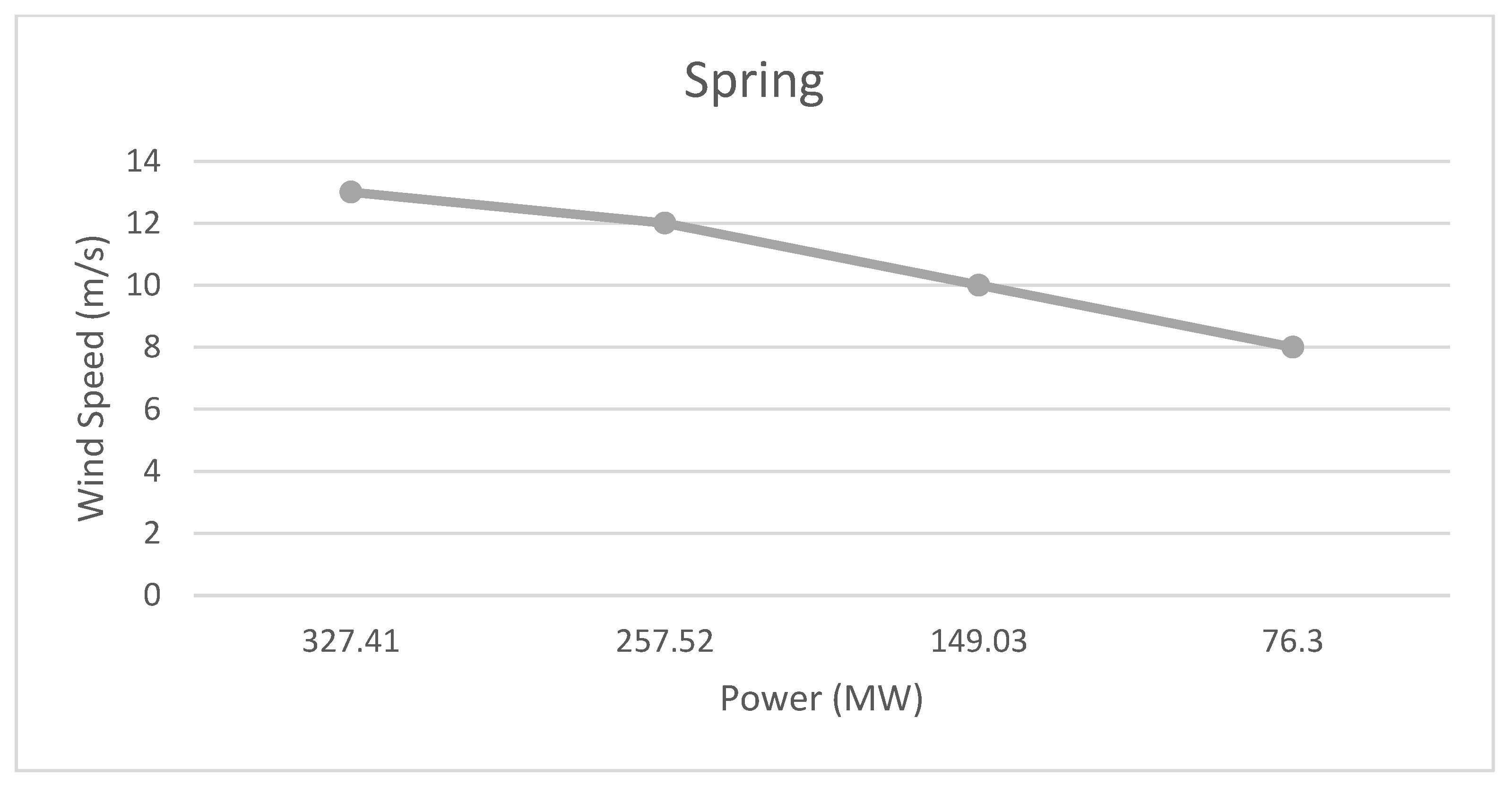
In spring, the wind speeds were more stable than in the winter and autumn seasons. In the first three days of the sample week for the spring season, the wind speed was 10 m/s. The subsequent days of the week had values that were almost identical to the first three days. On the fourth day, the wind speed increased slightly to 13 m/s; on the fifth day, it was 12 m/s. Because of this, the power prediction during this season will be more accurate due to the relatively stable wind speed.

In summer, it is noticed that the wind speed was stable with a decreased average speed in comparison to the other seasons. The wind speed on most days of the week sample was 8 m/s. This stability resulted in the increase in the accuracy of the wind forecast. Further, this low wind speed will provide less wind farm power compared to the other seasons.

The wind speed and power produced varied according to the seasons. To obtain a comprehensive understanding of the amount of power produced throughout the year, Figure 9 presents a visualization of the four seasons.

From Figure 9, it can be observed that the power production of the wind farm during the sample weeks was at a relatively stable level in the summer due to the consistency of the wind speeds. In autumn and spring, the power output was more variable, while in the winter, the variation in the power output increased even more due to the increasing variation in the wind speed.

6.2.2. Relationship between the Wind Speed and Power Production across the Four Seasons in Makkah, Considering the Wake Effect

The power output varied according to the wind speed; the higher the speed, the higher the power production.

Table 10. Power produced in the wind farm with five rotor spacings for the winter.

Date	Wind Max. Speed	Power of 256 Turbines in D1 (MW)	Power of 149 Turbines in D2 (MW)	Power of 111 Turbines in D3 (MW)	Power of 92 Turbines in D4 (MW)	Power of 81 Turbines in D5 (MW)
5/2/2017	18	870.4	870.16	872.46	868.48	864.27
6/2/2017	6	33.28	32.78	32.19	32.2	32.4
7/2/2017	12	258.56	257.77	258.63	257.6	255.96
8/2/2017	14	409.6	409.75	410.7	408.48	406.62
9/2/2017	12	258.56	257.77	258.63	257.6	255.96
10/2/2017	18	870.4	870.16	872.46	868.48	864.27
11/2/2017	7	51.2	50.66	51.06	50.6	51.03

shows the power production of one turbine from D1 to D5 for each of the wind speeds mentioned in the sample week of the four seasons.

In winter (Table 10), it is noted that the energy produced was uneven and unstable due to the considerable variation in the wind speed, as discussed before. This variation in the wind speed affected the power production in the different farm layouts (D1 to D5). It is noted that as the wind speed became slower, the power production was almost similar in the different farm layouts. For instance, on the second day, the wind speed was 6 m/s, with only a 1.1 MW difference between the maximum power production (33.28 MW) in D1 and the minimum power production (32.19 MW) in D3. Although, there was significant variation in the number of turbines between D1 and D5, the power productions from D1 to D5 were almost similar. With the increase in the wind speed, the difference in the energy produced between the five farm layouts (D1 to D5) increased. For example, in the winter, the difference between the farms with a wind speed of 18 m/s was 8.2 MW between the maximum and minimum power productions (872.46 and 864.27 MW).

In autumn (

Table 11. Power produced in the wind farm with five rotor spacings for the autumn.

Date	Wind Max. Speed	Power of 256 Turbines in D1 (MW)	Power of 149 Turbines in D2 (MW)	Power of 111 Turbines in D3 (MW)	Power of 92 Turbines in D4 (MW)	Power of 81 Turbines in D5 (MW)
8/5/2017	12	258.56	257.77	258.63	257.6	255.96
9/5/2017	13	327.68	327.8	328.56	327.52	325.62
10/5/2017	10	148.48	149	149.85	149.04	148.23
11/5/2017	5	17.92	19.37	18.87	18.4	18.63
12/5/2017	10	148.48	149	149.85	149.04	148.23
13/5/2017	10	148.48	149	149.85	149.04	148.23
14/5/2017	10	148.48	149	149.85	149.04	148.23

), the average wind speed was 10 m/s. D3 recorded the highest energy production, with 111 turbines, at wind speeds of 10, 12, and 13 m/s. The power produced reached 149.85 MW at a wind speed of 10 m/s in D3. On the other hand, D2 recorded the highest power production, with 149 turbines, at a wind speed of 5 m/s on the fourth day. At a 10 m/s wind speed, D5 recorded the lowest power production (148.23 MW), while at 5 m/s, D1 recorded the most insufficient power production (17.92 MW).

The spring season (

Table 12. Power produced in the wind farm with five rotor spacings for the spring.

Date	Wind Max. Speed	Power of 256 Turbines in D1 (MW)	Power of 149 Turbines in D2 (MW)	Power of 111 Turbines in D3 (MW)	Power of 92 Turbines in D4 (MW)	Power of 81 Turbines in D5 (MW)
5/8/2017	10	148.48	149	149.85	149.04	148.23
6/8/2017	10	148.48	149	149.85	149.04	148.23
7/8/2017	10	148.48	149	149.85	149.04	148.23
8/8/2017	13	327.68	327.8	328.56	327.52	325.62
9/8/2017	12	258.56	257.77	258.63	257.6	255.96
10/8/2017	8	76.8	75.99	76.59	76.36	76.14
11/8/2017	10	148.48	149	149.85	149.04	148.23

), was similar to autumn. The D3 wind farm recorded the highest power productivity on all days of the week, except for the sixth day. The average wind speed on most days was 10 m/s. D1 recorded the highest power production on the sixth day, with 256 turbines and a wind speed of 8 m/s. On the other hand, for the rest of the six days of the week, D3 recorded the best energy production with 111 turbines and wind speeds varying between 13 and 10 m/s.

In summer (

Table 13. Power produced in wind farm with five rotor spacings for spring.

Date	Wind Max. Speed	Power of 256 Turbines in D1 (MW)	Power of 149 Turbines in D2 (MW)	Power of 111 Turbines in D3 (MW)	Power of 92 Turbines in D4 (MW)	Power of 81 Turbines in D5 (MW)
4/11/2017	8	76.8	75.99	76.59	76.36	76.14
5/11/2017	8	76.8	75.99	76.59	76.36	76.14
6/11/2017	8	76.8	75.99	76.59	76.36	76.14
7/11/2017	8	76.8	75.99	76.59	76.36	76.14
8/11/2017	10	148.48	149	149.85	149.04	148.23
9/11/2017	8	76.8	75.99	76.59	76.36	76.14
10/11/2017	8	76.8	75.99	76.59	76.36	76.14

), the wind speed was 8 m/s on most days, except on the fifth day, it was 10 m/s. The power production was almost similar in all five layouts from D1 to D5 when the wind speed was 8 m/s; D1 recorded a slight increase in power production and reached 76.8 MW. The difference between the power prediction in the wind farms was approximately 0.8 MW at a wind speed of 8 m/s, while it was 1.6 MW at a wind speed of 10 m/s. This assures the notation that whenever the wind speeds increased, the variance of the power productivity increased from D1 to D5. From the power produced during the sample weeks (Table 13), it is observed that the power produced was uneven and unstable due to the considerable variation in the wind speed. On the first day during the sample week of the wind farm, the wind speed was monitored at 18 m/s, with a power production rate of 870 MW, while on the second day, it decreased to 6 m/s, which led to a decrease in the power produced in the farm to approximately 33 MW. Wind speeds were broadly similar during the sample weeks in autumn and spring. The average wind speed was 10 m/s, with an average power of approximately 149 MW. In the summer, the wind speed decreased somewhat steadily to 8 m/s per week of the sample, and the power produced was 76 MW.

7. Conclusions

The limitation of fossil fuel reserves and their disruption to the environment motivate renewable energy generation. The ever-increasing energy demand has drawn attention to renewable energy sources and other low-carbon, affordable energy sources for power generation due to the associated challenges, such the depletion of fossil fuel reserves, their price instability, and global climate change. In this work, five machine learning models were applied to predict wind farm power, namely, random forest regression, decision tree regression, gradient boosting regression, and linear regression. A case study concerning a city in Saudi Arabia included 1283 data points that were gathered from January 2015 to July 2018 from a wind station in Makkah. Further, the layout to produce a wind farm of 150 MW factoring the wake effect was considered. In the simulation studies, the wind speed had the most effect on the amount of power produced. In addition, decision tree regression was found to have the best accuracy values in all four used metrics, with 0.994 in R-squared, 0.025 in MAE, 0.273 in MSE, and 0.522 in RMSE, while the linear regression scored the least in all four metrics. In the setting and layout of a wind farm in Makkah, 52 SG 2.9-129 turbines were required to produce approximately 150 MW of power. When taking into account the wake effect, the number of wind turbines increased up to 81 turbines. Due to the convergence of wind speeds, energy production at the planned wind farm during the sample weeks was relatively stable in the summer season. However, due to the variability in the wind speeds, the power production fluctuated much more in the winter. The higher the wind speed, the more significant the difference in the energy production between the five farm layouts, and vice versa, whereas at a low wind speed, there was no significant difference in the power production in all of the near wake lengths of the 1D to 5D rotor diameters downstream from the rotor disc. The case study was conducted for Makkah, Saudi Arabia, and the obtained results were satisfactory and further provide support for the construction of several wind farms, producing hundreds of MWs in Saudi Arabia.