Investigation of the Splashing Characteristics of Lead Slag in Side-Blown Bath Melting Process

Abstract

Aiming at the melt splashing behavior in the smelting process of an oxygen-enriched side-blowing furnace, the volume of fluid model and the realizable $k$−$\epsilon$ turbulence model are coupled and simulated. The effects of different operating parameters (injection velocity, immersion depth, liquid level) on splash height are explored, and the simulation results are verified by water model experiments. The results show that the bubbles with residual kinetic energy escape to the slag surface and cause slag splashing. The slag splashing height gradually increases with the increase in injection velocity, and the time-averaged splashing height reaches 1.01 m when the injection speed is 160 m/s. Increasing the immersion depth of the lance, and the slag splashing height gradually decreases. When the immersion depth is 0.12 m, the time-averaged splashing height is 0.85 m. Increasing the liquid level is beneficial to reduce the splash height, when the liquid level is 2.7 m, the splash height reduces to 0.77 m. With the increase in the liquid level, the slag splashing height gradually decreases, and the time-averaged splashing height is 0.77 m when the initial liquid level is 2.7 m.

1. Introduction

In the field of metal smelting, oxygen-enriched bath melting technology is an advanced and efficient bath melting technique. During the metallurgical process, oxygen-rich air is blown through the lance into the molten pool and subsequently flows within the pool in the form of bubbles. The flow of oxygen-rich air not only provides oxidizing gas for the reaction in the melt pool, but also has an agitation effect on the melt pool. This melting method has the advantages of high energy utilization, rich oxygen concentration, producing less fumes, and good economic efficiency [1,2,3]. At present, according to different blowing methods, oxygen-enriched bath melting technology can be divided into bottom-blowing, side-blowing, and top-blowing according to different blowing methods, among which oxygen-enriched side-blowing bath melting furnace is widely used in continuous side-blowing bath melting of metals [4]. To meet the needs of industrial production, the immersion lance blows gas into the melt pool in the form of jet flow, which violently stirs up the flow of the hot melt. Due to the high velocity of the gas jet, the gas jet flow can significantly affect the chemical and physical processes in the furnace, such as oxidation reactions, gas–liquid mixing, and melt splashing. In particular, melt splashing is a concomitant phenomenon in the gas–liquid mixing process. Molten metal splashing can aggravate furnace lining refractory erosion, increase metal loss, cause tumors at the furnace mouth, and have a significant impact on the performance of side-blown melting furnaces [5,6,7,8]. Therefore, it is necessary to investigate the phenomenon of melt splashing within the side-blown furnace.

At present, owing to the extremely high temperature and poor visibility in the metallurgical melt pool, the gas–liquid two-phase flow in the melt pool is investigated mainly by two methods: water model experiments and numerical simulations. Therein, the water modeling method uses a liquid and a physical model of the metallurgical furnace to carry out the experiments. The water model experimental platform allows observation of gas flow patterns, penetration depths, splash heights, and other phenomena, which allows analysis of the flow field. Wang et al. [9]. investigated the factors affecting the diameter of bubbles in a bottom-blown copper melting furnace by building a water model platform. The results showed that increasing the installation angle of the lance would decrease the average diameter of the bubbles, and the diameter of the lance had a positive relationship with the average diameter of the bubbles. Shui et al. [10]. established a water model experimental platform for a bottom-blow copper smelting furnace with a single lance and examined the variation of gas and liquid mixing time by adjusting several operating parameters. The results showed that increasing the gas flow rate and the liquid level height of the melt pool in the stirring zone above the lance can effectively reduce the gas and liquid mixing time. However, increasing the liquid level decreases the mixing range of the gas. Wang et al. [11]. studied the influence of particles attached to the bubble surface on its deformation and oscillation during separation and floating. The results showed that the existence of particles on the interface significantly reduces the damping coefficient of bubble oscillation, which has little effect on the oscillation frequency. Bergamasco et al. [12]. made an in-depth analysis of the bubble oscillation process in fluids and demonstrated the existence of transient diffusion effects of bubbles with full equilibrium adaptation even at very low frequencies.

The method of water modeling experiments assists in the analysis of the flow field distribution in metallurgical furnaces. However, if the multi-physical fields such as turbulence field, velocity field, and temperature field in the metallurgical furnace are further analyzed, the numerical simulation method needs to be used. Abbassi et al. [13]. studied the effects of liquid viscosity, surface tension, and inertial force on the shape change during bubble floating. The results showed that the shape of bubbles was mainly affected by the surface tension and inertial force of the solution, and the viscosity had little effect on the shape change in the process of bubbles floating in the solution with low viscosity. Viscosity played a major role in the change in bubble shape in the solution with high viscosity. Wang et al. [14]. analyzed eight different oil–gas ratio working conditions in the Y-shaped feed pipe by a numerical calculation method. The results showed that at the oil–gas ratio of 1:2, the gas in the branch pipe was tangentially disturbed relative to the oil phase in the main pipe, and a cyclonic flow would be formed during the mixing descent in the vertical pipe. After the oil–gas mixture entered the melt pool, the annular gas–liquid mixing perturbation in the melt pool formed the best diffusion form of cyclonic diffusion. Liu et al. [15]. took the oxygen-enriched measuring and blowing furnace as the prototype, according to the similarity principle the water model was established and carried out the experiment. The experiments showed that the gas phase velocity has a great influence on the flow of the liquid phase, and the immersion depth of the lance has a relatively small effect on the penetration depth and surface fluctuation height in the liquid phase. They also compared the simulation results of three turbulence models, Standard $k-\epsilon$, realizable $k-\epsilon$, and SST $k-\omega$. The results showed that the realizable k − ε turbulence model was the closest to the experimental results. Xiao et al. [16]. proposed three improved gas injection methods of side-blowing molten bath: oblique, horizontal staggered, and vertical staggered, and compared the improvement effects of the three gas injection methods on the weak circulation area in the melt pool center through numerical simulation. The results showed that the oblique injection method had the best improvement effect and effectively reduced the amount of slag splashing in the molten bath.

However, there are significant differences in fluid properties between the laboratory-built experimental platform and the industrial high-temperature reactor, and the flow characteristics obtained in the cold experimental rig are not fully applicable to the industrial mixing process. In addition, the current research on computational fluid dynamics (CFD) simulation of metallurgical furnaces mainly focuses on the gas–liquid two-phase flow process in the melting furnace. Few scholars have studied the splashing phenomenon of molten metal in the side-blowing process, and the working parameters used to decrease the slag splashing in the side-blowing process are rarely reported [17,18,19,20,21].

To supplement the gap in this research direction, the volume of fluid (VOF) multiphase flow model and realizable $k-\epsilon$ turbulence model are coupled in this paper, and the splash process generated during the gas–liquid mixing is simulated. Firstly, a reasonable model of a side-blown melting furnace is established, and the simulation results of bubble morphology are verified by the water model experimental platform. Subsequently, the effect of three operating parameters (injection velocity, immersion depth, and liquid level height) on the time evolution of the slag splash height is investigated.

2. Model Establishment

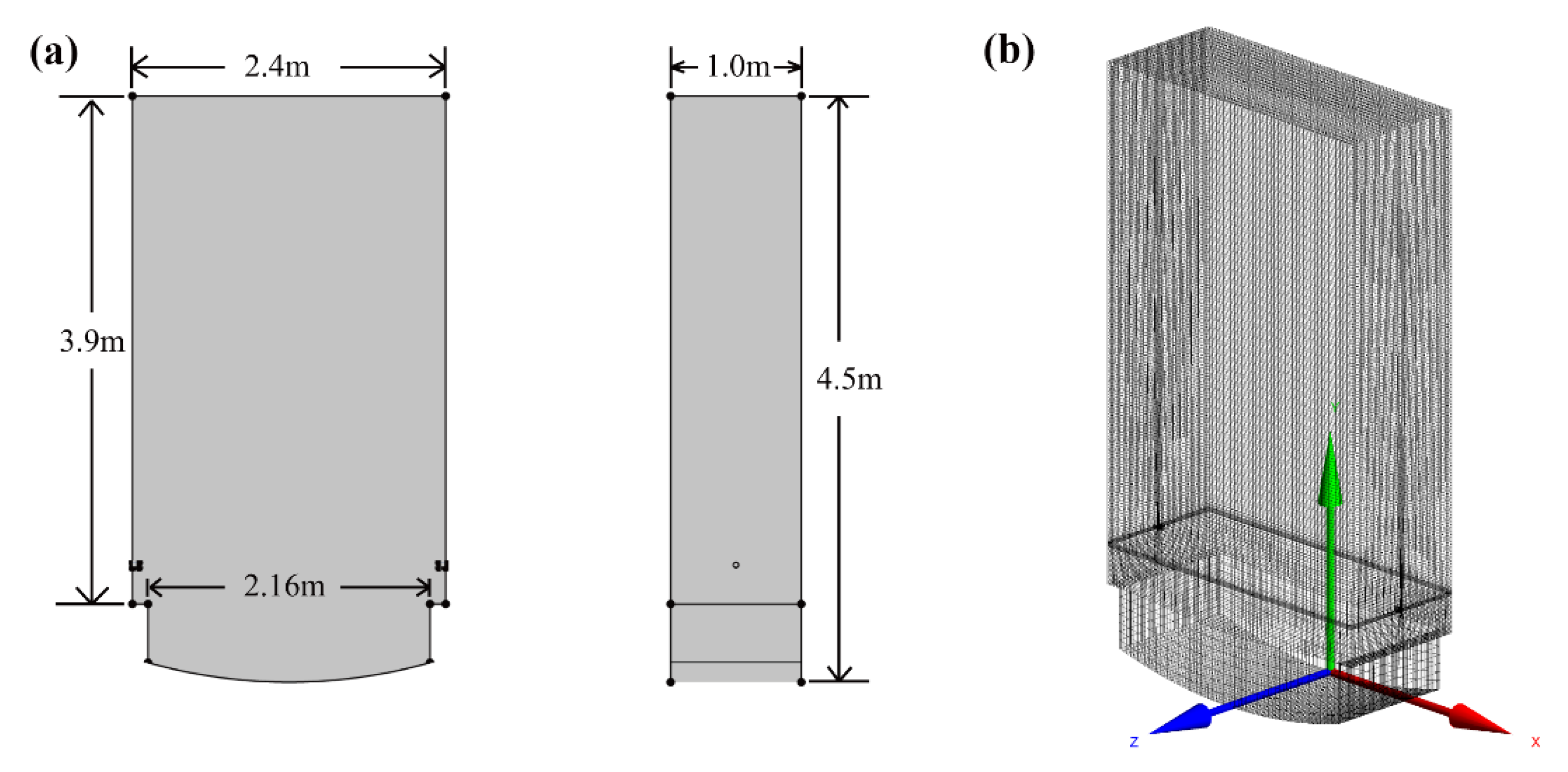
2.1. Physical Model

In this study, a side-blown melting furnace of a company in Huize County, China, was used as a simulation object. The construction of a complete side-blown melting furnace with multiple pairs of lances requires a huge number of meshes, which can be extremely burdensome for subsequent calculations. To ensure high calculation accuracy and appropriately reduce the number of grids, only a pair of lances is included in the calculation domain, and the sections on both sides of the lance are defined as periodic boundaries to consider the influence of other lances. The size and meshing diagram are shown in Figure 1a. The grid type selected for the calculation domain is hexahedral unstructured grid. To facilitate the description later, the coordinate system shown in Figure 1b is adopted. Considering that the two-phase flow area mainly occurs in the outlet area of the lance and the melt area above, the number of grids in these two parts is increased. Calculation parameters of the oxygen-rich side-blowing furnace are shown in

Table 1. The operating parameters selected in the simulation calculation.

Parameters	Values
Lance diameter	0.04 m
Lance height	0.9 m
Gas density	1.15 kg/m3
Gas viscosity	1.79 × 10−5 Pa*s
Slag density	2727 kg/m3
Slag viscosity	0.23 Pa*s

.

This paper mainly studies the bubble growth behavior and bubble flow behavior during the melting process of a submerged side-blown molten bath. Therefore, the following simplifications and assumptions are adopted in this study:

(1)

Disregarding the chemical reactions occurring in the melt bath;

(2)

The wall is regarded as a slip-free boundary, and the standard wall function is used to deal with the boundary layer near the wall;

(3)

The computational domain contains only one pair of nozzles and defines the cross sections on both sides of the nozzles as periodic boundaries;

(4)

It is assumed that the depth of the melt pool is constant. Discontinuous processes such as material addition, deslagging, and matte-making reaction are not considered.

2.2. Mathematical Model

2.2.1. VOF Model

VOF model is a surface tracking method based on a fixed Euler grid. The model tracks the phase interface by solving the continuity equation of multiphase volume fraction [22]. The volume fraction equation of phase $k$ is:

$$\frac{\partial {\alpha }_k}{\partial t}+v_k\cdot \nabla {\alpha }_k=\frac{S{\alpha }_k}{{\rho }_k}$$

(1)

The phase function is introduced to characterize the fraction of a phase medium occupying the grid area or volume, so as to realize fluid tracking. In the governing equation, the interface tracking between gas and liquid phases is described by solving the continuity equation of gas volume fraction. Assuming that the gas phase is the $k$ phase, the volume fraction equation is described as follows:

$$\frac{\partial {\alpha }_k}{\partial t}+v_k\cdot \nabla {\alpha }_k=\frac{S{\alpha }_k}{{\rho }_k}+\frac{1}{{\rho }_k}{\displaystyle {\sum }_{k=1}^n(m_{ik}-m_{ki})}$$

(2)

${\rho }_k$ is the density of $k$ phase; ${\alpha }_k$ is the volume fraction of $k$ phase; $v_k$ is the velocity of phase $k$; $m_{ik}$ is the mass transfer from $i$ phase to $k$ phase; $m_{ki}$ is the mass transfer from $k$ phase to $i$ phase; $S_{ak}$ is the source item.

The velocity field of VOF multiphase flow model is shared by all phases and obtained by solving a single momentum equation in the whole region. The momentum equation is as follows:

$$\frac{\partial }{\partial t}(\rho u)+\nabla (\rho uu)=-\nabla p+\nabla \left[\mu (\nabla u+\nabla u^T)\right]+\rho g+F$$

(3)

$\rho$ is the density of fluid; $u$ is the velocity of the fluid; $\mu$ is the viscosity of the fluid; $F$ is the volume force acting on the control volume.

2.2.2. Turbulence Model

The melting process in the metallurgical furnace is very complex. The turbulent flow in a molten bath has the characteristics of irregularity, unsteady, and dissipation [23]. There are many physical parameters in the turbulent flow field, such as pressure, kinetic energy, and so on. According to the existing research, the coupling result of realizable $k$ − $\epsilon$ turbulence model and VOF model is closer to the irregular motion in the metallurgical furnace, so the realizable $k$ − $\epsilon$ turbulence model is selected in this study. The general transport equations of $k$ and $\epsilon$ in the turbulence model are as follows:

Turbulent kinetic energy equation $k$:

$$\frac{\partial (\rho k)}{\partial t}+\nabla \cdot (\rho Uk)=\nabla \cdot ({\alpha }_k{\mu }_{eff}\nabla k)+G_k-\rho \epsilon$$

(4)

Turbulent energy dissipation rate equation $\epsilon$:

$$\frac{\partial (\rho \epsilon )}{\partial t}+\nabla \cdot (\rho U\epsilon )=\nabla \cdot ({\alpha }_k{\mu }_{eff}\nabla \epsilon )+C_{\epsilon 1}\frac{\epsilon }{k}{G}_k-C_{\epsilon 2}\rho \frac{{\epsilon }^2}{k}-R$$

(5)

where $R=\frac{\rho C_{\mu }{\eta }^3(1-\eta /{\eta }_0){\epsilon }^3}{1+\beta {\eta }^3}\frac{{\epsilon }^2}{k}$; $\eta$ is the ratio of the time scale of turbulence to the average stretch, and there $\eta =\frac{Sk}{\epsilon }$, $S={(2S_{ij}{S}_{ij})}^{1/2}={(G/{\mu }_e)}^{1/2}$; $G_k$ is the generation rate of turbulent kinetic energy; $B$ is the volume force; ${\alpha }_k$ and ${\alpha }_{\epsilon }$ is the turbulent Prandtl number of $k$ equation and $\epsilon$ equation; ${\mu }_{eff}$ is the effective viscosity, as shown below:

$${\mu }_{eff}=\mu +{\mu }_i$$

(6)

$${\mu }_i=C_{\mu }\rho \frac{k^2}{\epsilon }$$

(7)

where $\mu$ is dynamic viscosity; turbulent kinetic energy is $k=0.5\overline{u_i{u}_j}$, turbulent dissipation rate $\epsilon =\mu \frac{\overline{u_i{u}_j}}{\partial x_i\partial y_j}$; $C_{\epsilon 1}$, $C_{\epsilon 2}$, $C_{\mu }$ are empirical constants, respectively.

2.2.3. Physical Parameters Setting

In this study, all fluids are regarded as incompressible fluids. The energy equation is ignored, that is, the heat transfer is not considered; the atmospheric pressure of the external environment is 101,325 Pa and the gravitational acceleration is 9.81 m/s². The inlet boundary condition is given velocity-inlet, the inlet is air with volume fraction of 1, and the outlet boundary condition is pressure outlet.

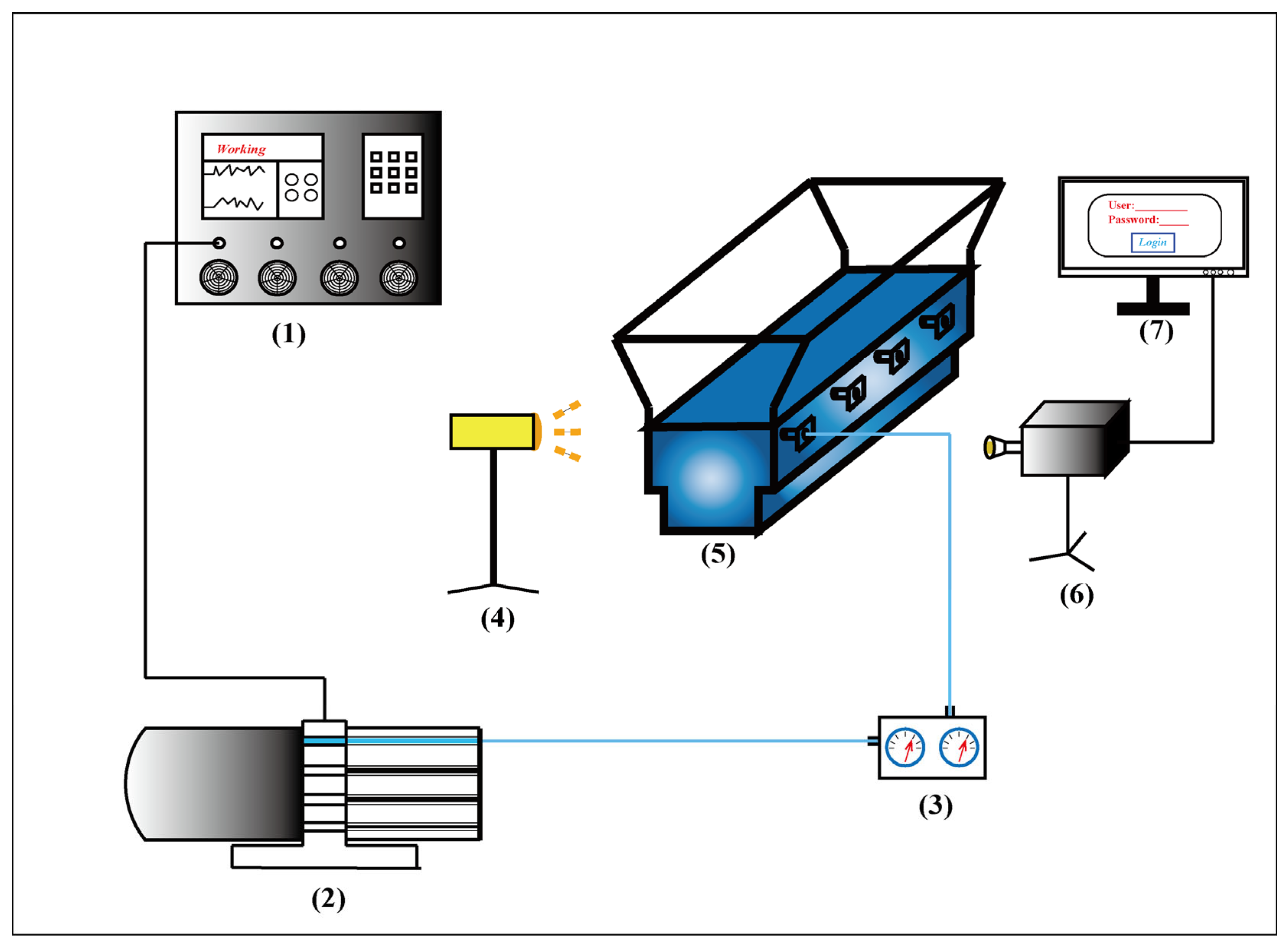
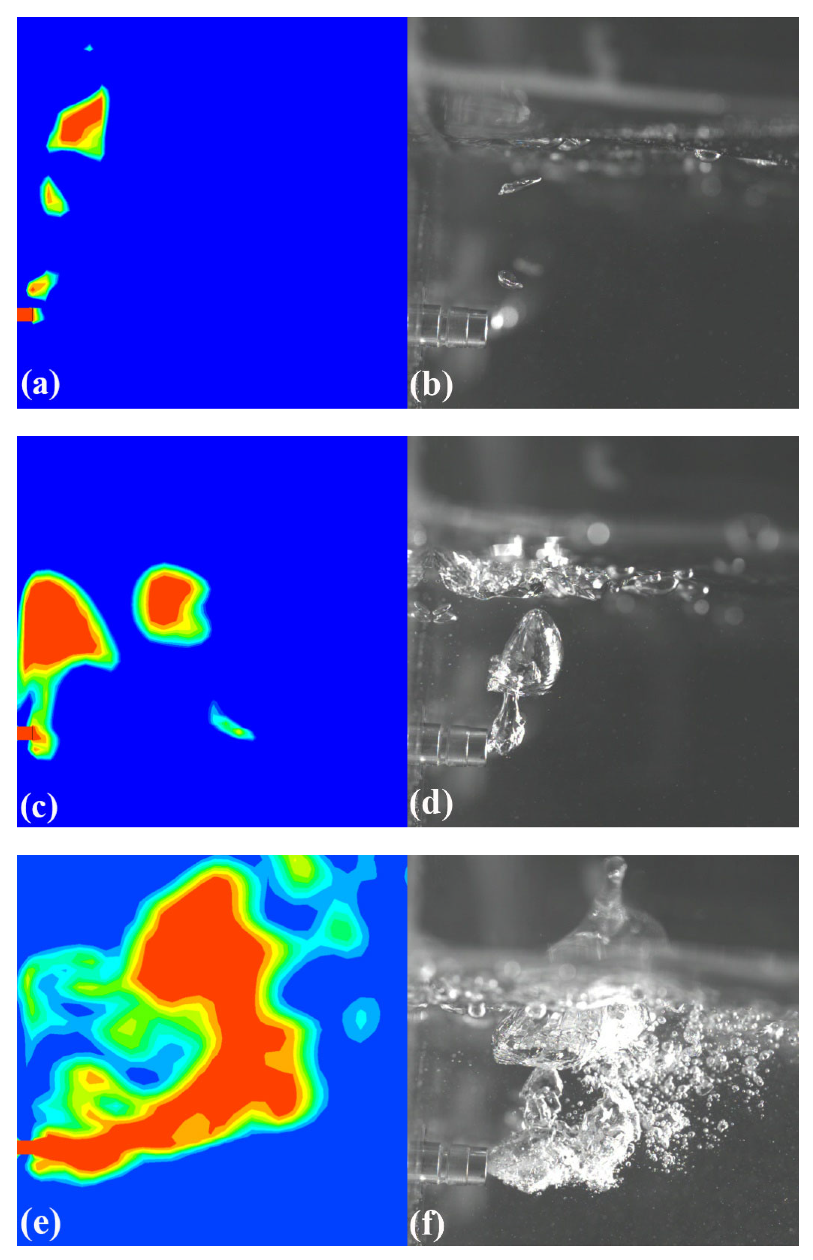
3. Experimental Validation of Numerical Models

In the process of bubble floating, the buoyancy force, inertia force, and shear stress are dynamic changes, and the interaction between the bubble and the surrounding slag makes the morphology of the bubble change rapidly [10,15,18,24]. To ensure the credibility of the simulation results, this section compares the experimentally obtained bubble flow behaviors with the simulated bubble flow behaviors to verify the accuracy and precision of the numerical model. The constructed experimental platform for water model validation is shown in Figure 2.

The water model experimental platform built in this section has a similarity ratio of 1:2 to the 3D side-blown furnace designed in this paper. In the experiment, different lance flow rates are set by the control center so that the flow pattern of the air stream is bubbly, slug-like, and emulsion-like, respectively. Figure 3 shows the comparison of the bubble morphology between the simulation results (Figure 3a,c,e)) and the experimental results (Figure 3b,d,f)) for different lance flow rates(1 L/min, 3 L/min, and 9 L/min). When the flow rate of the gas injected by the lance is 1 L/min, the flow pattern of the bubble flow is bubble-like flow, which is characterized by the regular generation of bubbles. The generation of bubbles has a certain periodicity and there is no interaction between bubbles. Increasing the lance flow rate to 3 L/min, the bubble flow shape changes to a slug flow, which is characterized by the phenomenon that different bubbles begin to break and coalesce with each other continuously. The volume of the coalesced bubbles increases significantly, which increases the plume effect of the bubbles and makes the subsequent bubbles elongate. As the lance flow rate increases to 9 L/min, the flow pattern of bubbles changes to emulsion flow. This flow pattern is characterized by the continuous aggregation of bubbles near the nozzle and the increased continuity of the bubble flow. The simulation results are slightly different from the experimental results, mainly due to slight fluctuations in the gas injection rate during the experiment and the vibration of the lance during the injection. Overall, the simulated three working conditions validate the bubble morphology and flow characteristics compared to the experimental results. It shows that the VOF model coupled with the realizable $k-\epsilon$ model is reliable in describing the mixed gas–liquid flow in the side-blown melting furnace.

4. Simulation Results and Analysis

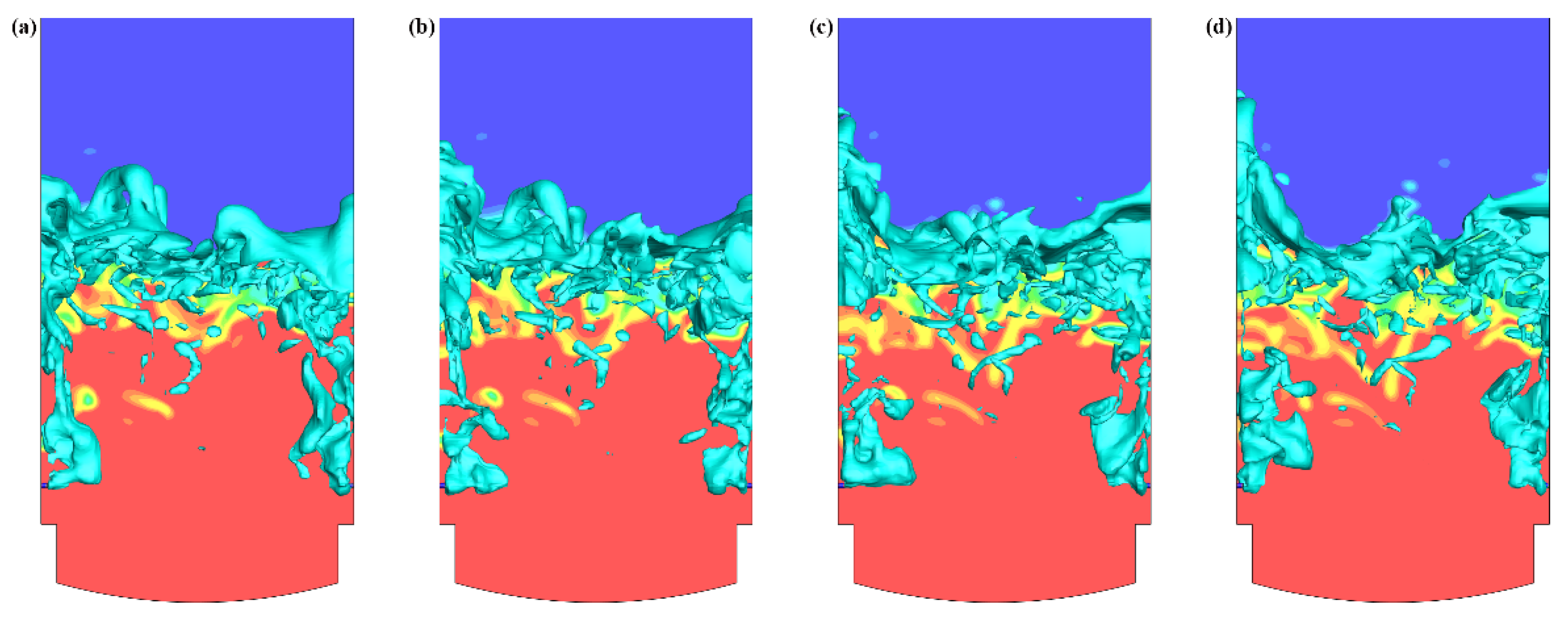
4.1. Analysis of Slag Splashing Causes

The slag splashing process is shown in Figure 4. In the side blow melting process, gas is injected into the melt pool as a high-velocity jet. After the high-velocity jet enters the melt pool, bubbles are formed at the lance outlet due to the resistance of the melt. At the same time, the initially stationary melt in the lance outlet area begins to flow. The bubbles are broken into larger and smaller bubbles by the shear stress applied during the melt flow. Smaller bubbles get caught in the slag, increasing the gas content of the slag layer and improving the melting efficiency. The larger bubbles begin to float upward under the influence of buoyancy and eventually escape from the melt pool. The bubbles still have residual kinetic energy when escaping from the molten pool, so the bubbles carry the slag with them out of the slag surface. Eventually, the bubble breaks and causes the slag to spray. For the convenience of the following description, the instantaneous splashing height of the slag and the initial liquid level height of the molten pool are defined as the splashing height.

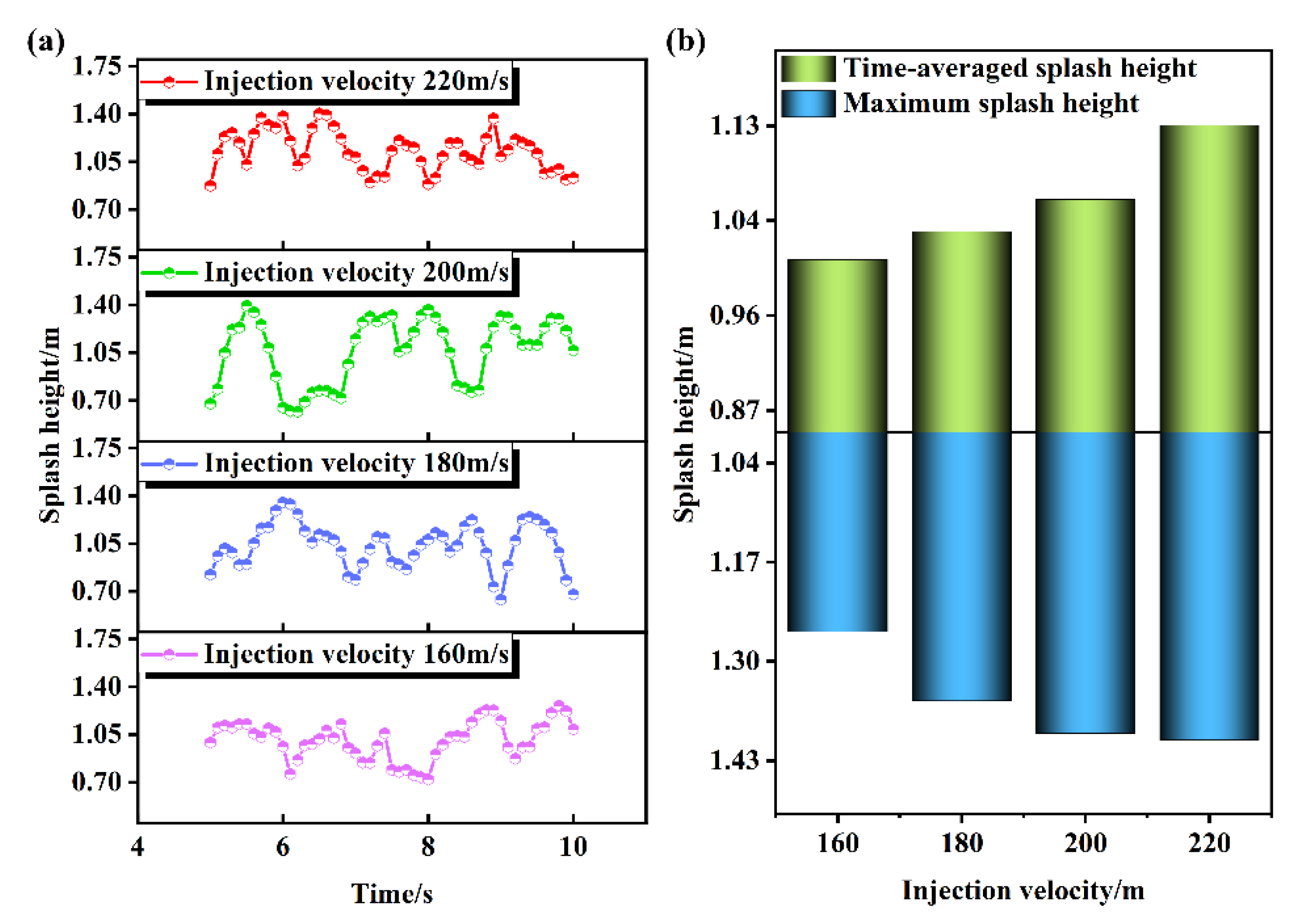
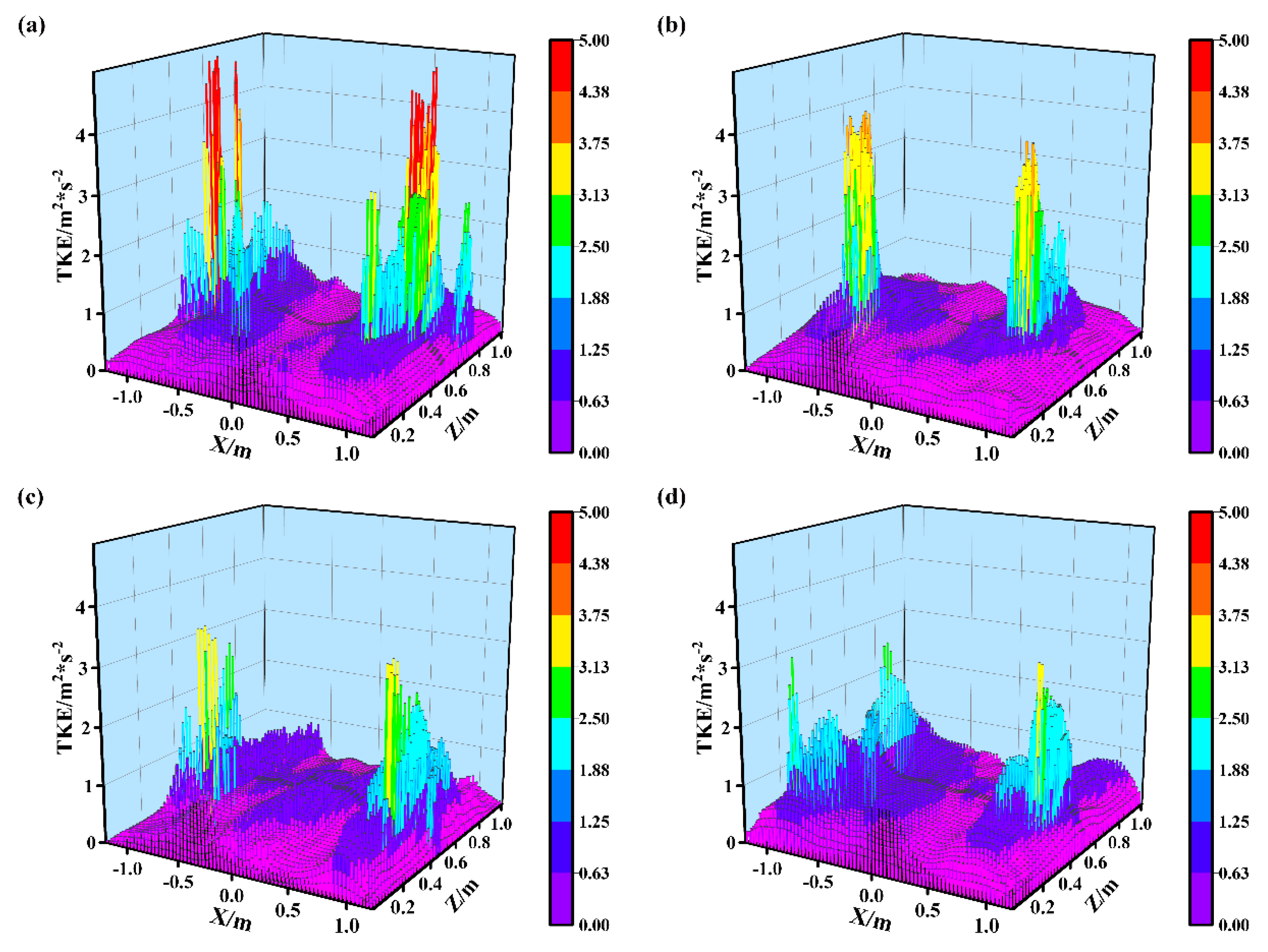
4.2. Influence of Gas Injection Velocity on Splash Height

A numerical simulation of a three-dimensional lead melting side-blown furnace was carried out using the above-mentioned calculation method. To illustrate the influence of different gas injection velocities on the slag splashing height, four working conditions were constructed to change the injection velocity of the side-blowing lance. The parameters of the four working conditions are shown in

Table 2. Parameters of different injection velocity working condition groups.

Condition	Injection Speed (m/s)	Immersion Depth (m)	Liquid Level (m)
1	160	0.04	2.5
2	180	0.04	2.5
3	200	0.04	2.5
4	220	0.04	2.5

.

When the melt pool reached dynamic equilibrium, the instantaneous splash height, time-averaged splash height, and maximum splash height of the slag are counted, respectively, and the results are shown in Figure 5.

From Figure 5a in working conditions 1 to 4, the splash height of the slag fluctuates within a certain range and shows a trend of periodic variation. Meanwhile, the splash height variation of the melt exhibits a “multi-peak” characteristic. This indicates that splashing occurs more frequently in the melt pool and causes continuous scouring of the upper furnace lining material by the slag. Meanwhile, the splash height within the melt pool fluctuates widely, which indicates poor overall stability within the melt pool.

From Figure 5b, the average splash height of the melt pool is 1.01 m, 1.03 m, 1.06 m, and 1.13 m with the increase in the injection velocity. Obviously, by increasing the injection velocity, the average splash height of the slag increases as well. This is due to the low initial kinetic energy carried by the gas when the lance blows at a lower velocity. As the lance injection velocity increases, the initial kinetic energy carried by the gas increases, and the residual kinetic energy of the bubble at the time of escape is higher. As a result, the time-average splash height gets higher.

The maximum splash height reflects the worst-case condition when the splash phenomenon occurs for the specified operating conditions. The complex flow of the slag makes the absorption of the bubble energy by the slag not fixed. The bubbles may transfer a minor amount of kinetic energy to the melt during the uplifting process. This leads to more kinetic energy remaining when the bubble escapes from the slag, which ultimately causes a dramatic increase in the single splash height. For working conditions 1 to 4, the maximum splash heights of the melt pool are 1.26 m, 1.35 m, 1.39 m, and 1.40 m, respectively. The maximum splash height also shows a pattern of increasing with the increase in the injection velocity. This shows that increasing the injection velocity will not only increase the average splash height, but the maximum splash height will also increase. The furnace lining in the upper part of the bath is more susceptible to slag erosion.

The process of bubble uplifting is accompanied by the transfer of kinetic energy, which gradually decreases for the bubble and increases for the melt. The kinetic energy remaining after the bubble rises to the liquid surface has a large influence on the splash height of the melt. Therefore, it is necessary to further investigate the turbulence kinetic energy (TKE) distribution within the melt pool.

To quantitatively analyze the TKE distribution in the melt pool, the average TKE data for the section y = 2.5 m shown in Figure 6 were extracted. The results are shown in Figure 7. For working condition 1, the TKE distribution in the melt pool shows a distribution pattern of large on both sides and small in the middle. The region of higher TKE is concentrated around the uplift path of the bubbles. This is due to the fact that the bubble’s uplift path is close to the wall of the melt pool, and the slag fails to absorb the kinetic energy of the bubble well. Meanwhile, in Figure 7a, most of the regions have TKE < 0.5 m²/s². It indicates that the turbulence intensity is low in most areas of the melt pool, the mobility of the slag in the melt pool is weak, and the gas is not effective in stirring the melt pool.

For working condition 2, the TKE distribution pattern in the melt pool still shows the distribution pattern of large on both sides and small in the middle. Compared to working condition 1, the slag around the bubble uplift path in working condition 2 has a higher TKE. This indicates that more kinetic energy is absorbed by the slag around the bubble uplift path in working condition 2. Meanwhile, by comparing Figure 7b and Figure 7a, there is a significant reduction in the area of TKE < 0.5 m²/s² in the melt pool. This indicates a certain improvement in the range of kinetic energy transfer within the melt pool. Additionally, the poor mobility of the slag has been improved.

For working condition 3, the area of higher turbulent energy in the melt pool is not concentrated at the walls of the two sides of the melt pool, but gradually approaches the middle of the melt pool. As the lance injection velocity increases, the bubble uplift path begins to shift away from the melt pool wall. This leads to an increase in the contact surface area between the bubbles and the slag, which is able to absorb more of the kinetic energy carried by the bubbles. Therefore, the maximum TKE of the slag in working condition 3 is significantly increased compared to working condition 2. The area of TKE > 0.5 m²/s² in the melt pool also increases significantly. The slag that absorbs the kinetic energy of the bubbles better transfers the kinetic energy to the slag in the area without bubble stirring, resulting in a more uniform distribution of kinetic energy in the melt pool.

For working condition 4, the maximum turbulent energy in the melt pool is more concentrated. The TKE distribution shows a “bimodal” shape with small peaks at both sides and large peaks in the middle. This indicates that the bubbles transfer more kinetic energy to the slag as the injection velocity increases. At the same time, there are fewer areas with TKE < 0.5 m²/s² in the melt pool, which effectively improves the mixing effect of the melt pool. This indicates that the bubbles transfer more kinetic energy to the slag as the injection velocity increases. However, increasing the injection velocity leads to the high initial kinetic energy of the bubbles, resulting in a large kinetic energy when the bubbles escape from the slag. Eventually, the splash height of the melt pool increases considerably.

Therefore, as the injection velocity increases, the residual kinetic energy is greater when the bubble escapes, and the average splash height of the melt pool gradually increases. The average splash height of the slag is the lowest at injection velocity of 160 m/s, which is 1.01 m. However, by increasing the injection velocity, the transfer range of kinetic energy in the melt pool is larger, and the region with larger turbulent kinetic energy moves from the two sides of the melt pool to the middle of the melt pool. Although this is effective in improving the fluidity of the slag and intensifying the mixing effect of the melt pool, it needs to suffer the effects of excessive slag splash heights. Considering the long-term negative impact of slag splash on the melt pool, the splash height of the slag should be limited during the actual production process. Therefore, the lance can be set to an injection velocity of about 160 m/s.

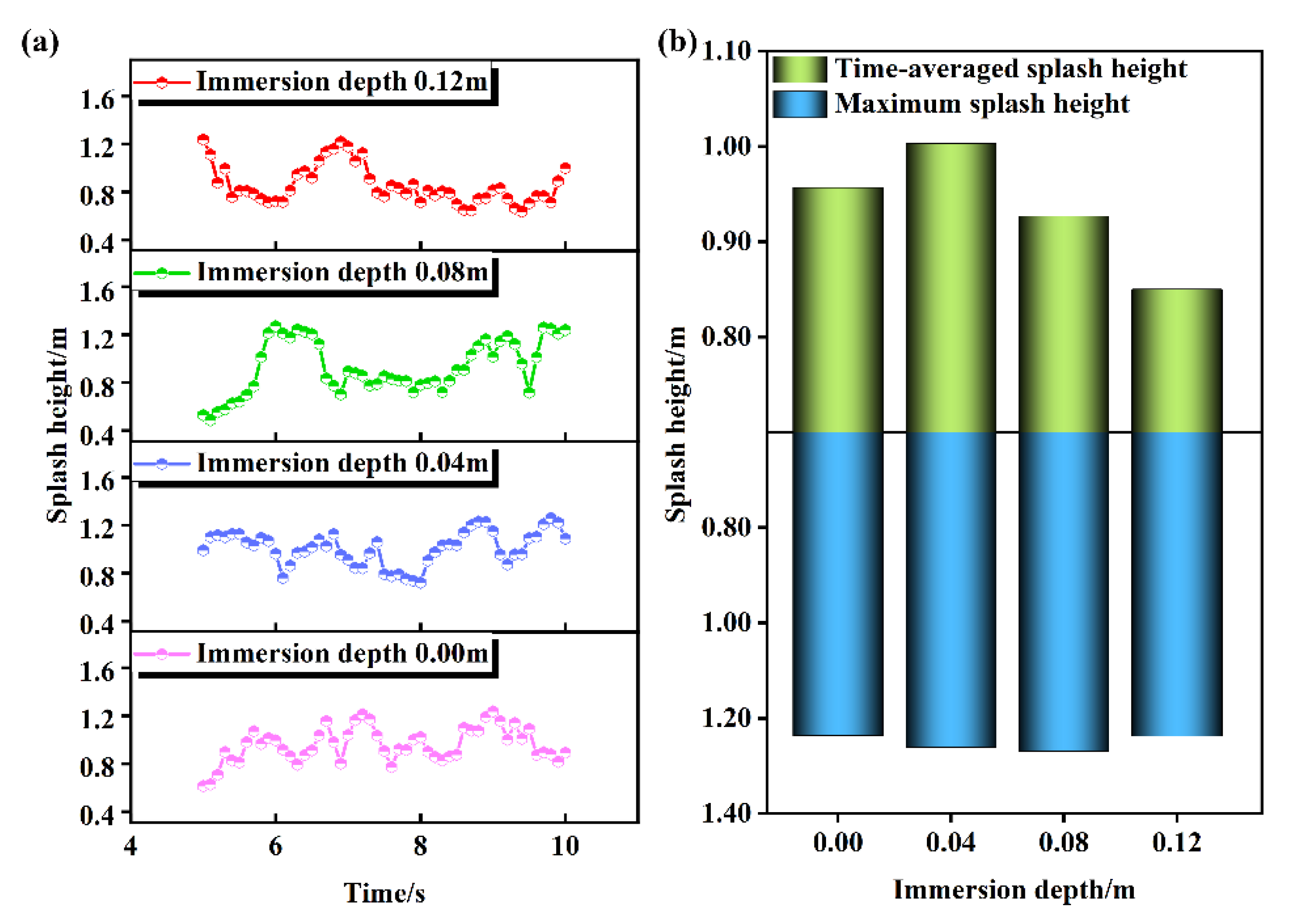
4.3. Effect of Lance Immersion Depth on Splash Height

To illustrate the effect of different lance immersion depths on the slag splash height, four working conditions are constructed, varying the immersion depth of the side blow lance. At the same time, considering the research content of Section 4.2, the injection velocity of the lance is set to 160 m/s in this section. The specific parameters are shown in

Table 3. Parameters of different immersion depth working condition groups.

Condition	Injection Speed (m/s)	Immersion Depth (m)	Liquid Level (m)
5	160	0.00	2.5
6	160	0.04	2.5
7	160	0.08	2.5
8	160	0.12	2.5

.

The variation of splash height with time and the average splash height for the four different immersion depth conditions are counted separately. Since the parameters of working condition 6 are the same as those of working condition 3, the data obtained are also identical. The specific results are shown in Figure 8.

As can be seen from Figure 8a, at a submerged depth of 0.00 m, the lance is non-submerged at this time. The specific splash height curve of the slag has a “multi-peak” distribution, which indicates a high frequency of splash phenomena. When the lance is submerged, the deeper the immersion depth of the lance, the lower the frequency of splash of the slag. This indicates that increasing the immersion depth of the lance can improve the stability of the melt pool.

As shown in Figure 8b, the time-average splash heights of the melt pool are 0.96 m, 1.01 m, 0.93 m, and 0.85 m with increasing immersion depth. The time-average splash height shows a pattern of increasing followed by decreasing. For working condition 5, as the lance is not submerged, the bubbles are tightly attached to the molten pool wall during the uplifting process due to the wall attachment effect [25,26]. This causes the bubbles to scour the furnace lining in the process of floating, thus consuming part of the kinetic energy carried by the bubbles. Therefore, the slag splashing height is low when the non-submerged injection method is adopted. For the lance using the submerged mode of operation, changing the submerged depth of the lance, the starting position of the bubble uplift also changes. In comparison with working conditions 6 and 5, the time-average splash height of the slag is higher at a submergence depth of 0.04 m. This is attributed to the fact that the bubble’s uplifting path becomes farther away from the molten pool wall, and the kinetic energy consumption caused by the bubble scouring the furnace lining is reduced, so the remaining kinetic energy when the bubble escapes increases. With the further increase in the immersion depth, the starting position of the bubble floating is closer to the middle of the melt pool, and the kinetic energy consumed by the bubble scouring the wall of the furnace is further reduced. However, it would increase the contact area between the bubble and the slag, and the slag would be able to absorb more kinetic energy carried by the bubble. Therefore, the time-averaged splash height of the slag gradually decreases as the immersion depth of the lance increases.

Observing Figure 8b, the maximum splash heights of slag for working conditions 5 to 8 are 1.24 m, 1.26 m, 1.27 m, and 1.24 m, respectively. Apparently, the maximum splash height of the slag hardly varies after changing the immersion depth of the lance. In comparison with Figure 5b, the maximum splash height of the slag is proportional to the initial kinetic energy carried by the high-speed airflow into the molten pool, independent of the immersion depth of the lance, for the same initial liquid level of the molten pool. It means that the immersion depth of the lance does not affect the maximum kinetic energy that may remain when the bubble escapes.

Similarly, to further investigate the TKE distribution of the splashing process, the average turbulent kinetic energy data of the y = 2.5 m section were extracted, and the results are shown in Figure 9.

It can be observed in Figure 9 that the turbulent kinetic energy distribution of working condition 5 has the characteristics of overall small and local large. Slag with high TKE is scattered near the walls of the furnace. This is since the lance in working condition 5 is non-submerged, which allows the bubbles to take an uplifting path within the slag close to the furnace wall. The bubbles can only transfer kinetic energy to the slag near the wall, which in turn makes this part of the slag with a high TKE. Comparing the turbulence energy distribution characteristics of the four working conditions, the maximum turbulence energy in the melt pool is about 3.2 m²/s². This means that if only the immersion depth of the lance is changed, the amount of kinetic energy transferred by the bubbles to the slag is almost the same, and the maximum TKE that the slag may hold is almost the same. That also clearly explains why there is minimal variation in the maximum splash height from working conditions 5 to 8.

However, as the immersion depth increases, the bubble uplifting starts closer to the middle of the melt pool, which makes the bubble uplifting process closer to the middle of the melt pool as well. Comparing working conditions 6, 7, and 8, the TKE in the middle of the melt pool in working condition 6 is weak, which indicates that the mobility of this part of the slag is extremely poor, and the stirring effect of bubbles on this part of the slag is close to none. In working condition 7, the turbulent energy of the slag in the center of the melt pool is significantly increased, which has improved the flow of the melt pool. In working condition 8, the slag flow in the center of the melt pool is significantly improved, which leads to a significant improvement of the gas–liquid mixing effect in the melting process.

To sum up, changing the immersion depth of the lance mainly affects the start of bubble uplifting. As the blowing speed increases, the time-average splash height of the slag decreases. Meanwhile, the weak flow region in the center of the melt pool gradually decreases, and the turbulence intensity of the slag increases significantly. However, changing the immersion depth of the lance has no effect on the maximum splash height. Therefore, by comparing the average splash height, the immersion depth of the lance can be set at about 0.12 m.

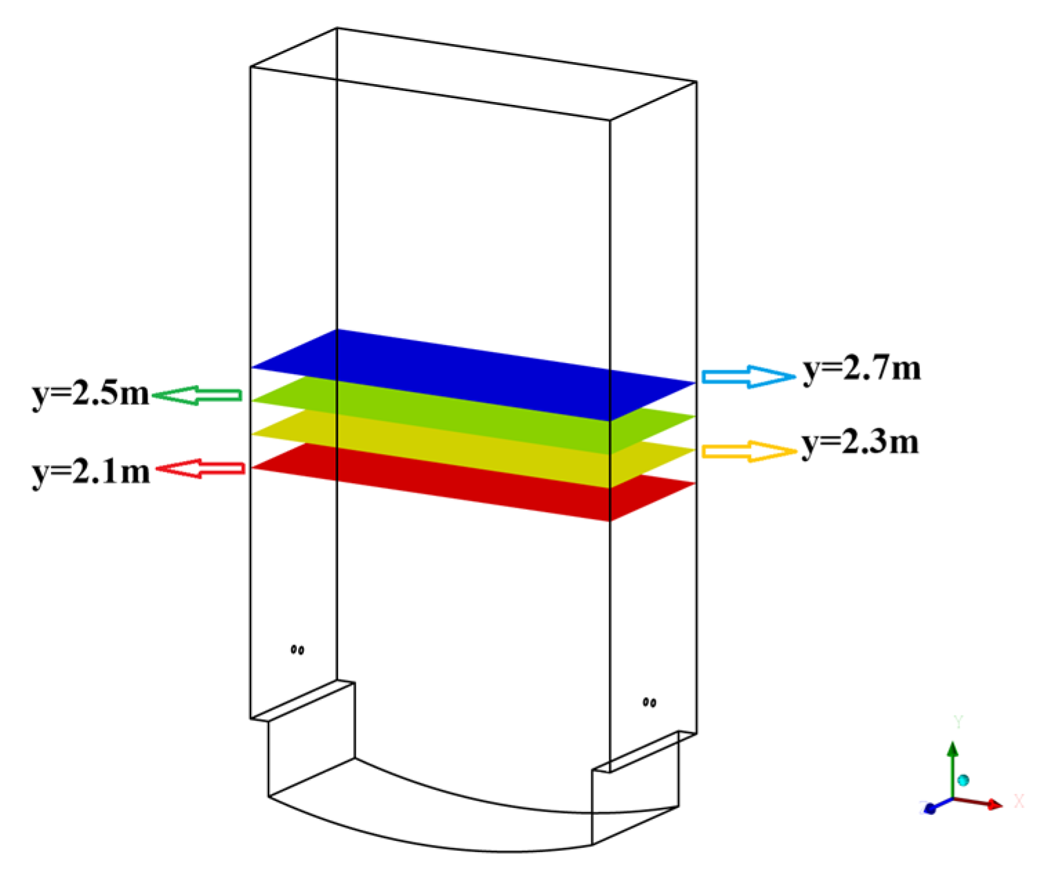
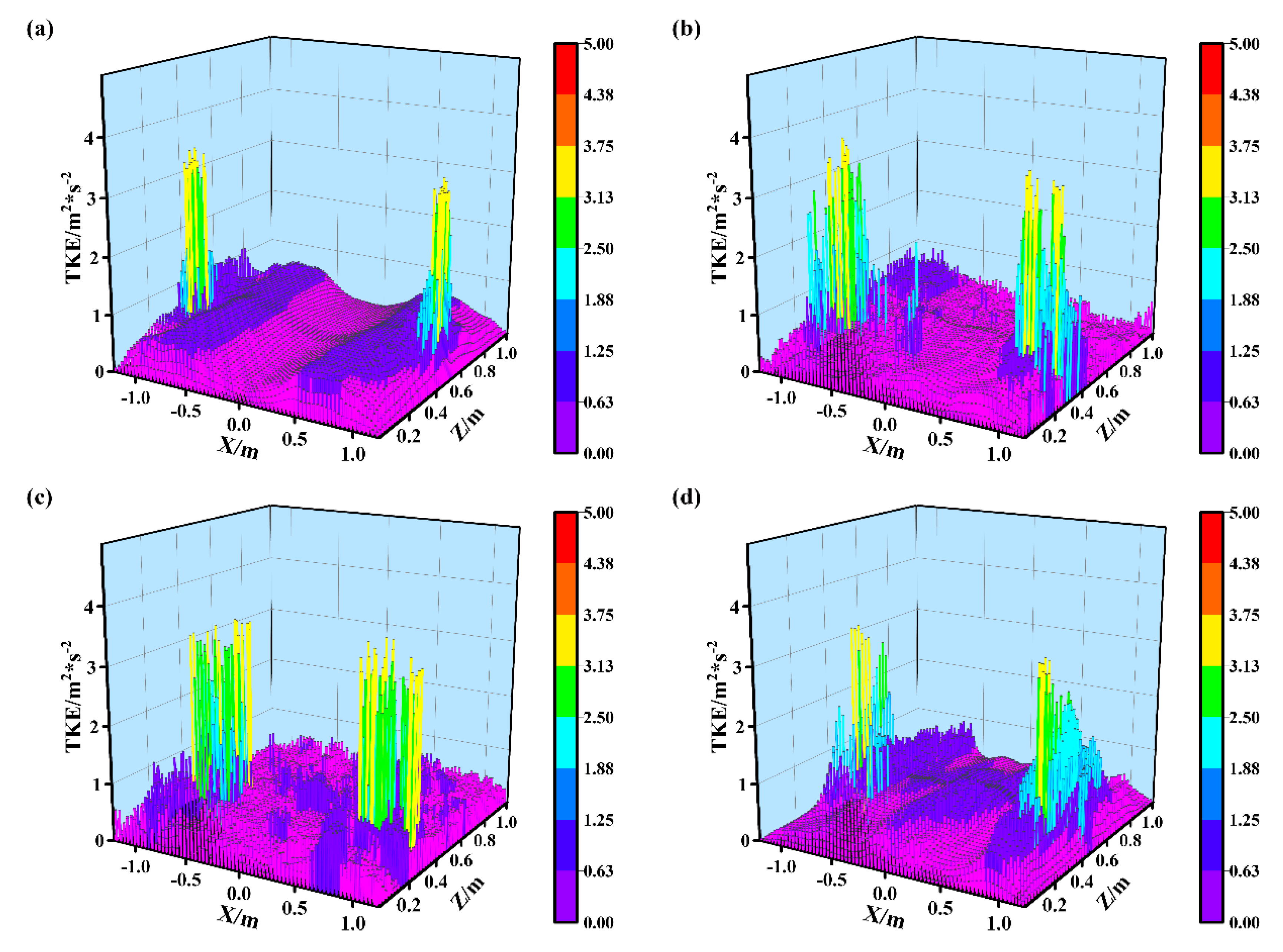
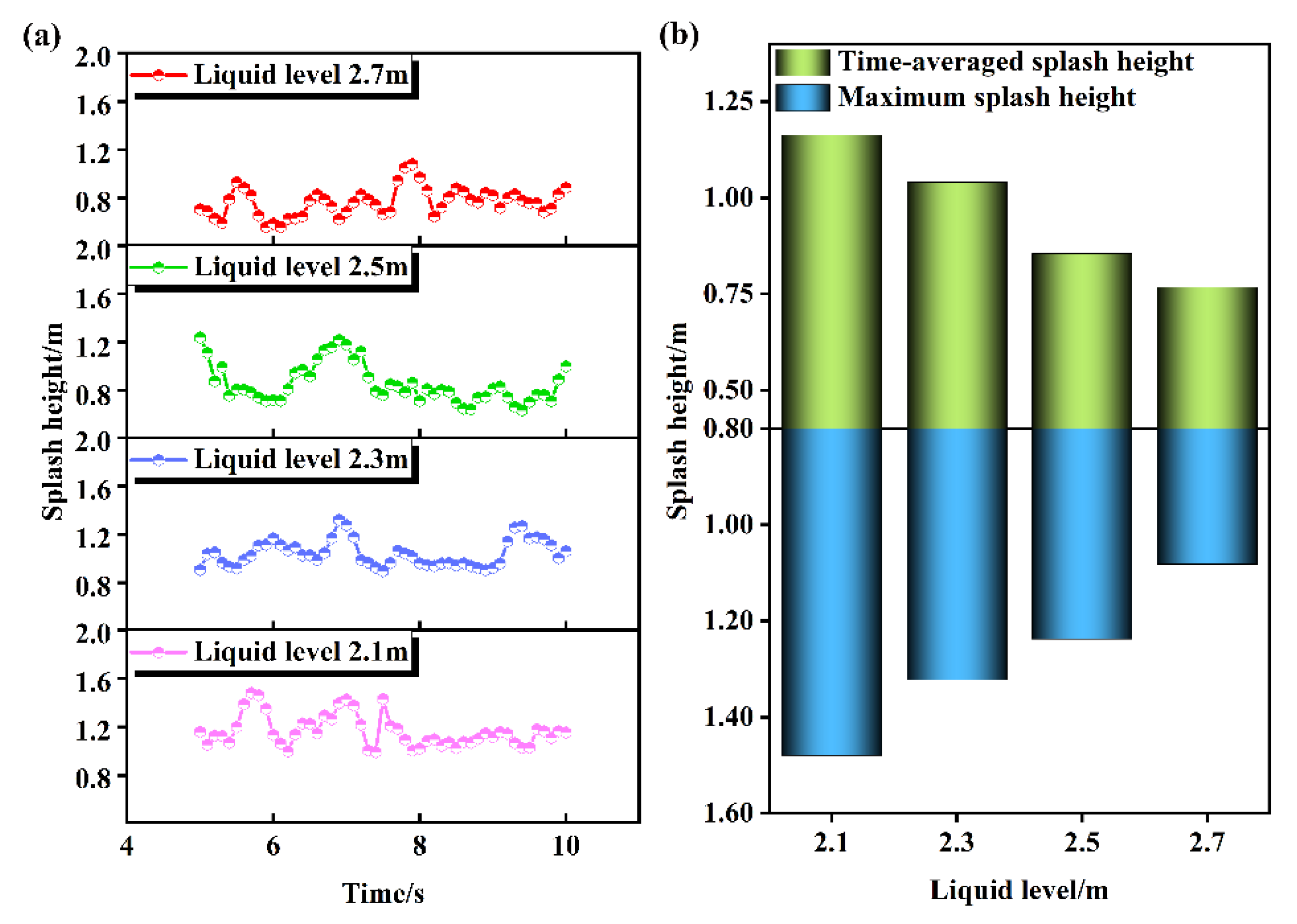
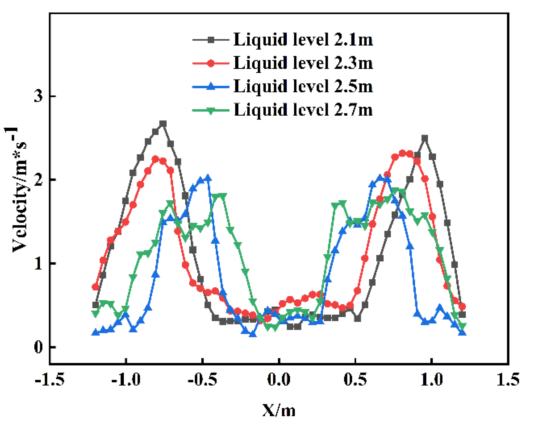
4.4. Effect of Initial Liquid Level on Splash Height

To illustrate the effect of different initial liquid level heights on the splash height of the slag, four working conditions are constructed, varying the initial liquid level of the molten pool. Meanwhile, considering the research content of Section 4.2 and Section 4.3, the injection velocity of the lance is set to 160 m/s in this chapter, and the immersion depth of the lance is set to 0.12 m. The specific parameters are shown in

Table 4. Parameters of different liquid level working condition groups.

Condition	Injection Speed (m/s)	Immersion Depth (m)	Liquid Level (m)
9	160	0.12	2.1
10	160	0.12	2.3
11	160	0.12	2.5
12	160	0.12	2.7

.

The splash height variation with time and the average splash height are counted separately for the four different working conditions mentioned above. Since the parameters of working conditions 11 and 8 are the same, the obtained data and conclusions are completely identical. The results are shown in Figure 8.

Observing Figure 10a, the initial liquid level height of the melt pool is low for working conditions 9 and 10. The splashing height of slag is kept at a high value for a long time. On the contrary, in working conditions 11 and 12, the slag splash height is kept at a low value for a prolonged period of time in the working conditions with a high initial liquid level height of the melt pool. This indicates that changing the initial liquid level of the melt pool has a significant effect on the variation of the splash height of the slag.

According to Figure 10b, with the increase in the liquid level, the time-average splashing height of slag is 1.16 m, 1.04 m, 0.85 m, and 0.77 m, respectively. The maximum splash heights of the slag are 1.48 m, 1.32 m, 1.24 m, and 1.08 m, respectively. Obviously, both the time-averaged and maximum splash heights decrease as the initial liquid level grows. Increasing the initial liquid level of the melt pool could extend the length of the bubble uplift path. The longer the uplift path, the more contact time between the slag and the bubbles. For working conditions 9 and 10, the time-averaged and maximum splash heights are large for both conditions. This is due to the short uplift path of the bubbles, which in turn leads to insufficient contact time between the bubbles and the slag, and the bubbles still have a high velocity when escaping from the slag surface. Figure 11 shows the velocity of the bubbles when they float up to the initial liquid level for working conditions 9 to 12. In the exploration conditions, the distribution of velocity shows an “inverted W” distribution. The maximum velocities for the four working conditions are 2.67 m/s, 2.32 m/s, 2.02 m/s, and 1.88 m/s, respectively. Obviously, increasing the initial liquid surface height can effectively extend the upward path length of the bubbles. Further, it would increase the contact time between bubbles and slag and reduce the velocity of bubbles when escaping. Ultimately, the effect of slag splash suppression is achieved.

Similarly, to further investigate the TKE field distribution in the melt pool, TKE data are extracted for the section where the initial liquid level is located from working conditions 9 to 12. The results are shown in Figure 12.

As shown in Figure 12, the maximum TKE in the melt pool decreases significantly with the increase in the initial liquid level of the melt pool. Compared to working condition 11, working conditions 9 and 10 have a lower initial liquid level, and the maximum TKE of the slag is distributed between 3.5 m²/s² and 5 m²/s². Obviously, the slag stirring intensity in the upper part of the melt pool is stronger in working conditions with lower initial liquid levels. This is due to the large kinetic energy maintained by the bubbles as they flow through the region at a higher velocity. Accordingly, more kinetic energy is absorbed by the surrounding slag. Additionally, for working conditions 11 and 12, the maximum TKE of working condition 12 is distributed between 2 m²/s² and 3 m²/s². The increase in the initial liquid level height allows a longer path for the bubbles to rise within the slag. The velocity and kinetic energy of the bubbles are substantially reduced when they reach the upper part of the melt pool after a longer uplifting path. Therefore, the kinetic energy that can be absorbed by the slag in the upper part of the melt pool is reduced. This indicates that the splash phenomenon of the slag is improved by increasing the initial liquid level. However, the stirring intensity of the slag in the upper part of the melt pool is also reduced accordingly.

5. Conclusions

In this research, numerical simulations are conducted to investigate the slag splash characteristics in an oxygen-rich side-blown lead-melting furnace. The mathematical models of the VOF multiphase model and realizable $k-\epsilon$ viscous model are coupled at first, and then the accuracy of the mathematical models is verified by the constructed experimental platform. The slag splash process in the melt pool with multiple working conditions is finally simulated in Fluent software. The effects of injection velocity, immersion depth, and initial liquid level are investigated comparatively. We conclude the following conclusions:

(1)

The slag cannot absorb all the kinetic energy of the bubbles during the floating process.

(2)

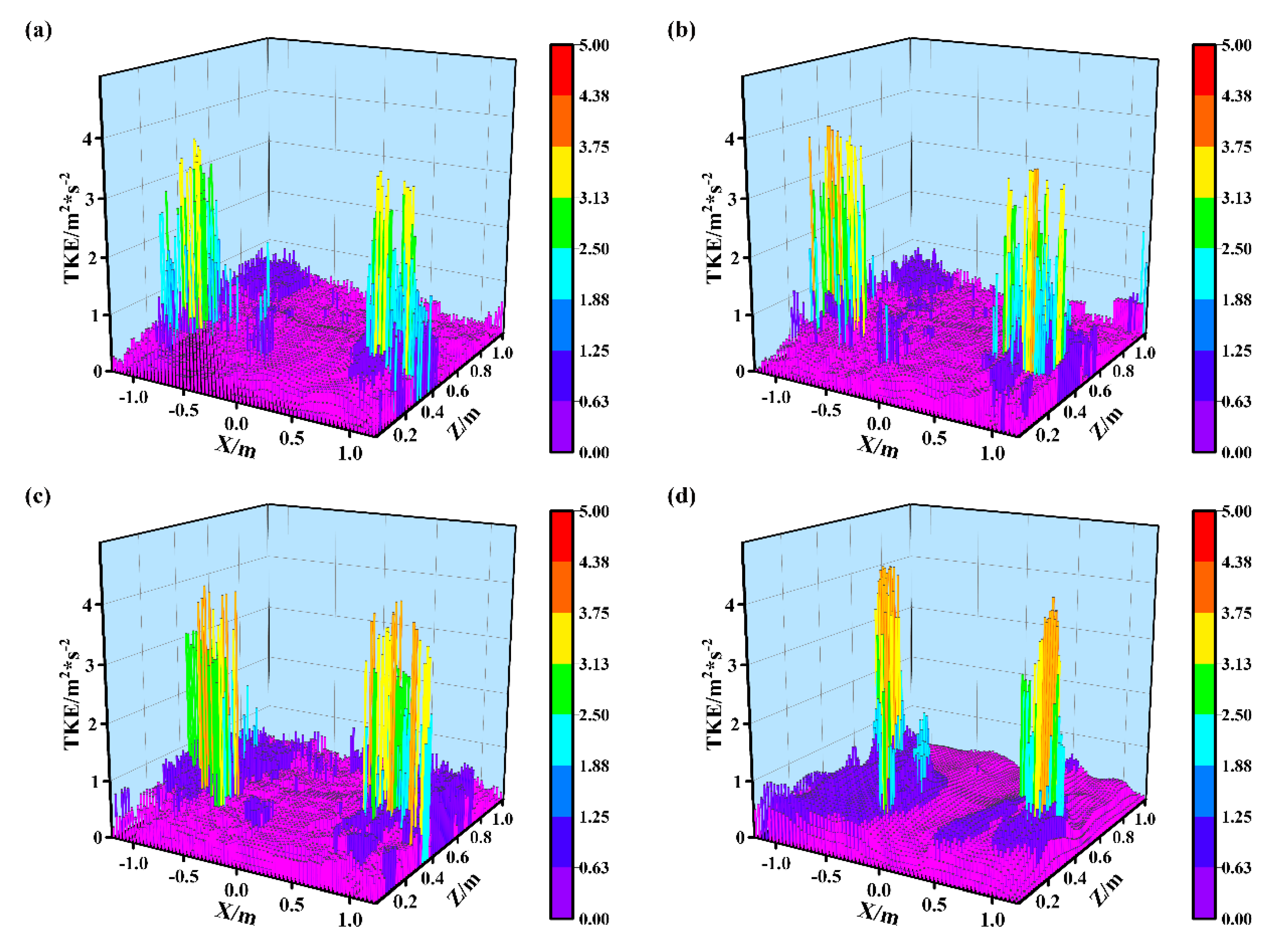
As the injection velocity increases, the time-averaged splash height and the maximum splash height of the slag increase. The time-average splash height of the slag is 1.01 m, and the maximum splash height is 1.26 m with 160 m/s injection velocity of the lance. Meanwhile, the maximum TKE of the slag increases with the growth of the injection velocity, and the mobility of the slag in the center of the melt pool gradually improves.

(3)

The time-averaged splash height of the slag increases and then decreases as the immersion depth increases, while the maximum splash height remains almost unchanged. The time-averaged splash height of the slag is 0.85 m, and the maximum splash height is 1.24 m with a 0.12 m immersion depth of the lance. Increasing the immersion depth of the lance has no effect on the maximum TKE of the slag but enhances the mobility of the slag in the center of the melt pool.

(4)

As the initial liquid level increases, both the time-averaged splash height and the maximum splash height of the slag decrease gradually. At the initial liquid level of 2.7 m, the time-averaged splash height of the slag is 0.77 m, and the maximum splash height is 1.08 m. The maximum TKE of the slag decreases significantly with the growth of the initial liquid level.

References

1. Liu, F.H.; Sun, D.B.; Zhu, R.; Dong, K.; Bai, R.G. Effect of Side-blowing Arrangement on Flow Field and Vanadium Extraction Rate in Converter Steelmaking Process. ISIJ Int. 2018, 58, 852–859. [Google Scholar] [CrossRef] [Green Version]
2. Zhong, L.C.; Zhou, X.B.; Zhu, Y.X.; Chen, B.Y.; Huang, B.C.; Ke, J.X. Industrial Experiment of Steelmaking in a Top-Bottom-Side Blown Converter with Slag Splashing Process. Steel Res. Int. 2012, 83, 16–21. [Google Scholar] [CrossRef]
3. Zhou, X.B.; Ersson, M.; Zhong, L.C.; Jonsson, P.G. Numerical and Physical Simulations of a Combined Top-Bottom-Side Blown Converter. Steel Res. Int. 2015, 86, 1328–1338. [Google Scholar] [CrossRef]
4. Zhong, L.C.; Wang, X.; Zhu, Y.X.; Chen, B.Y.; Huamg, B.C.; Ke, J.X. Bath mixing behaviour in top-bottom-side blown converter. Ironmak. Steelmak. 2010, 37, 578–582. [Google Scholar] [CrossRef]
5. Li, L.; Li, M.; Li, Q.; Zou, Z. Melt splashing behavior of steelmaking converter with nozzle-twisted lance. Iron Steel 2020, 55, 54–60. [Google Scholar]
6. Mills, K.C.; Su, Y.C.; Fox, A.B.; Li, Z.S.; Thackray, R.P.; Tsai, H.T. A review of slag splashing. ISIJ Int. 2005, 45, 619–633. [Google Scholar] [CrossRef] [Green Version]
7. Santos, I.A.S.; Santos, V.R.D.; Lima, W.D.; da Silva, A.L.; Maia, B.T.; de Oliveira, J.R. Slag Splashing: Simulation and analysis of the slags conditions. J. Mater. Res. Technol. JMRT 2019, 8, 6173–6176. [Google Scholar] [CrossRef]
8. Yang, T.Z.; Xiao, H.; Chen, L.; Chen, W.; Liu, W.F.; Zhang, D.C. Element Distribution in the Oxygen-Rich Side-Blow Bath Smelting of a Low-Grade Bismuth-Lead Concentrate. JOM 2018, 70, 1005–1010. [Google Scholar] [CrossRef]
9. Wang, D.X.; Liu, Y.; Zhang, Z.M.; Shao, P.; Zhang, T.A. Dimensional Analysis of Average Diameter of Bubbles for Bottom Blown Oxygen Copper Furnace. Math. Probl. Eng. 2016, 2016, 8. [Google Scholar] [CrossRef] [Green Version]
10. Shui, L.; Cui, Z.X.; Ma, X.D.; Rhamdhani, M.A.; Nguyen, A.; Zhao, B.J. Mixing Phenomena in a Bottom Blown Copper Smelter: A Water Model Study. Metall. Mater. Trans. B-Proc. Metall. Mater. Proc. Sci. 2015, 46, 1218–1225. [Google Scholar] [CrossRef]
11. Wang, H.; Brito-Parada, P.R. Shape deformation and oscillation of particle-laden bubbles after pinch-off from a nozzle. Chem. Eng. J. 2021, 412, 10. [Google Scholar] [CrossRef]
12. Bergamasco, L.; Fuster, D. Oscillation regimes of gas/vapor bubbles. Int. J. Heat Mass Transf. 2017, 112, 72–80. [Google Scholar] [CrossRef] [Green Version]
13. Abbassi, W.; Besbes, S.; El Hajem, M.; Aissia, H.; Champagne, J.Y.; Jay, J. Influence of operating conditions and liquid phase viscosity with volume of fluid method on bubble formation process. Eur. J.Mech. B-Fluids 2017, 65, 284–298. [Google Scholar] [CrossRef]
14. Wang, Y.H.; Wang, S.B.; Wei, Y.G.; Zhang, T.F.; Li, S.W. Numerical simulation of gas-liquid mixed top blowing to enhance momentum diffusion. Appl. Therm. Eng. 2020, 181, 12. [Google Scholar] [CrossRef]
15. Liu, Y.T.; Yang, T.Z.; Chen, Z.; Zhu, Z.Y.; Zhang, L.; Huang, Q. Experiment and numerical simulation of two-phase flow in oxygen enriched side-blown furnace. Trans. Nonferrous Met. Soc. China 2020, 30, 249–258. [Google Scholar] [CrossRef]
16. Xiao, Y.D.; Lu, T.T.; Zhou, Y.G.; Su, Q.Q.; Mu, L.Z.; Wei, T.; Zhao, H.L.; Liu, F.Q. Computational Fluid Dynamics Study on Enhanced Circulation Flow in a Side-Blown Copper Smelting Furnace. JOM 2021, 73, 2724–2732. [Google Scholar] [CrossRef]
17. Chang, S.; Zou, Z.S.; Liu, J.H.; Isac, M.; Cao, X.K.E.; Su, X.F.; Guthrie, R.I.L. Study on the slag-metal interfacial behavior under the impact of bubbles in different sizes. Powder Technol. 2021, 387, 125–135. [Google Scholar] [CrossRef]
18. Ma, J.; Zhou, P.; Cheng, W.; Song, Y.P.; Shi, P.Y. Dimensional analysis and experimental study of gas penetration depth model for submerged side-blown equipment. Exp. Therm. Fluid Sci. 2016, 75, 220–227. [Google Scholar] [CrossRef]
19. Sinelnikov, V.; Szucki, M.; Merder, T.; Pieprzyca, J.; Kalisz, D. Physical and Numerical Modeling of the Slag Splashing Process. Materials 2021, 14, 19. [Google Scholar] [CrossRef]
20. Valencia, A.; Rosales-Vera, M.; Orellana, C. Fluid Dynamics in a Teniente Type Copper Converter Model with One and Two Tuyeres. Adv. Mech. Eng. 2013, 5, 902874. [Google Scholar] [CrossRef] [Green Version]
21. Zhu, Z.; Zhou, P.; Chen, Z.; Long, P.; Zhang, L. Numerical simulation on effect of air injection on two-phase flow in oxygen-enriched side-blown furnace. J. Cent. South Univ. Sci. Technol. 2022, 53, 398–408. [Google Scholar]
22. Mulbah, C.; Kang, C.; Mao, N.; Zhang, W.; Shaikh, A.R.; Teng, S. A review of VOF methods for simulating bubble dynamics. Prog. Nucl. Energy 2022, 154, 20. [Google Scholar] [CrossRef]
23. Wang, Z.; Liu, W. Effects of near-wall turbulence model on numerical simulation of turbulent separated flows. Acta Aerodyn. Sinica 2002, 20, 198–205. [Google Scholar]
24. Singh, R.I.; Brink, A.; Hupa, M. CFD modeling to study fluidized bed combustion and gasification. Appl. Therm. Eng. 2013, 52, 585–614. [Google Scholar] [CrossRef]
25. He, X.; Zhu, X.; Yang, S.; Deng, Z. Coanda effect of flat taper pipe applied in valveless piezoelectric micro-pump. J. Harbin Inst. Technol. 2015, 47, 92–97. [Google Scholar]
26. Kitagawa, A.; Denissenko, P.; Murai, Y. Effect of wall surface wettability on collective behavior of hydrogen microbubbles rising along a wall. Exp. Therm. Fluid Sci. 2017, 80, 126–138. [Google Scholar] [CrossRef]
Figure 1. Schematic of computational domain (a) and mesh (b) used in simulation.
Energies 16 01007 g001
Figure 2. Schematic diagram of water model experimental platform: 1—console; 2—air pumps; 3—flow detector; 4—fill light; 5—water model experimental furnace; 6—high-speed camera; 7—image processing server.
Energies 16 01007 g002
Figure 3. Comparison of simulation results (a,c,e) and experimental results (b,d,f) for 3 different flow regimes of airflow during side-blown flow.
Energies 16 01007 g003
Figure 4. Profile of slag splash height process: (a) t = 6.10 s, (b) = 6.15 s, (c) = 6.20 s, (d) = 6.25 s.
Energies 16 01007 g004
Figure 5. Splash height at different injection velocities (a) instantaneous distribution of splash height; (b) time-averaged splash height and maximum splash height.
Energies 16 01007 g005
Figure 6. Schematic diagram of four sections.
Energies 16 01007 g006
Figure 7. TKE distribution on y = 2.5 m section, (a) injection velocity 160 m/s; (b) injection velocity 180 m/s; (c) injection velocity 200 m/s; (d) injection velocity 220 m/s.
Energies 16 01007 g007
Figure 8. Splash height at different immersion depths (a) instantaneous distribution of splash height; (b) time-averaged splash height and maximum splash height.
Energies 16 01007 g008
Figure 9. TKE distribution on y = 2.5 m section, (a) immersion depth 0.00 m; (b) immersion depth 0.04 m; (c) immersion depth 0.08 m; (d) immersion depth 0.12 m.
Energies 16 01007 g009
Figure 10. Splash height at different liquid levels (a) instantaneous distribution of splash height; (b) time-averaged splash height and maximum splash height.
Energies 16 01007 g010
Figure 11. Velocity of bubbles floating to the initial liquid level.
Energies 16 01007 g011
Figure 12. TKE at different initial liquid level, (a) liquid level 2.1 m; (b) liquid level 2.3 m; (c) liquid level 2.5 m; (d) liquid level 2.7 m.
Energies 16 01007 g012