Calibration of a Near-Wall Differential Reynolds Stress Model Using the Updated Direct Numerical Simulation Data and Its Assessment

Abstract

In the article, a differential Reynolds stress model is recalibrated using turbulent channel flow direct numerical simulation data in the range of friction Reynolds numbers 550–5200. The calibration aims to produce a RANS sublayer model for use within the hybrid RANS/LES framework. The model is designed to capture the average field of a thin near-wall part of a boundary layer as accurately as possible. An a posteriori procedure is employed in which one-dimensional channel flow calculations are performed for all variations of the model coefficients at each stage of the optimization procedure. The coefficients are initialized with their original values and then optimized by minimizing the appropriately chosen norm. An improved representation of the mean velocity profile and peak Reynolds stress values is demonstrated. Both models—baseline and recalibrated—are implemented in an in-house CFD code, and several simulations, including a channel flow, a flat plate boundary layer and a boundary layer separation from a rounded step, are performed. The latter benchmark flow is also simulated in hybrid RANS/LES mode. The updated model is compared to the original one, demonstrating improvements over the baseline model in the cases it was designed for.

1. Introduction

Differential Reynolds stress models (DRSM), which emerged in the middle of the 20th century [1,2], currently represent a very promising approach to turbulence modeling [3]. The main reasons for this are the recognition of restrictions imposed by the eddy viscosity models and DRSMs’ potential for improved prediction of flow separation, which is often relevant in practical applications [4].

The first DRSM to acquire widespread popularity was the Launder–Reece–Rodi (LRR) model [5,6]. The LRR model assumes a common approximation of the redistribution term, which is linear concerning the Reynolds stress tensor. A more general approximation that is quadratic with respect to the Reynolds stress tensor was suggested by Lumley [7], and its particular case simplification was proposed in the Speziale–Sarkar–Gatski (SSG) model [8]. Combining these two models and transitioning from the equation for the dissipation rate of turbulence kinetic energy $\epsilon$ to an equation for the turbulence frequency $\omega$ led to the creation of the SSG/LRR-ω model [9,10]. It became popular due to adopting concepts from a successful eddy viscosity model SST [11], a relatively simple model formulation and a reasonable level of accuracy in practical external aerodynamic applications [12]. It is worth noting that although the SSG/LRR-ω model suggests integrating the equations to wall and setting the no-slip boundary condition (with a demand that the first near-wall cell height correspond to $y_1^{+}\le 1$ in law-of-the-wall variables), this model cannot be considered accurate for detailed description of the near-wall portion of the boundary layer (such models are called “low-Reynolds-number models”). The model does not contain near-wall corrections to the redistribution term, and the dissipation rate tensor is assumed to be isotropic. This leads to substantial deviations of the Reynolds stress $R_{ij}=\overline{u_i{u}_j}$ (the overbar denotes a Reynolds average and $u_i$ is a fluctuating part of the $i$-th velocity vector component) and $\epsilon$ profiles from reference data.

Although the development of low-Reynolds-number DRSMs is a relatively niche research area, several prominent papers have been published on this topic. A large amount of work in this direction was put in by the Manchester University group led by B.E. Launder. In a span of two decades (1978–1998), they described several models in papers [13,14,15,16] and presented the final results of their research in the paper by T.J. Craft [17] in 1998. A group led by K. Hanjalić has been developing their low-Reynolds-number model since 1994; they proposed two models [18,19] and summarized their findings in the work of Jakirlić and Hanjalić [20], which was devoted to their JHh model of 2002. Subsequently, the model [20] became a basis for more practice-oriented low-Reynolds-number models JHh-v1, 2, 3 [10,21,22], in which efforts were made to empirically improve the prediction of separated flows and to account for the large-scale unsteadiness. The JHh model formulation was also used in the JH-${\omega }^h$ [23] and Jakirlić & Maduta [24] models, in which the $\omega$-equation is utilized, leading to improved computational stability. Another direction of low-Reynolds-number DRSMs is being developed by the group of G.A. Gerolymos (Pierre and Marie Curie University, Paris) [25,26]; their latest developed model, GLVY [27], was published in 2014.

The creation of hybrid Reynolds-averaged Navier–Stokes/Large Eddy Simulation (RANS/LES) methods is of particular interest in which a RANS turbulence model is only used in a thin near-wall layer [28]. In contrast, the outer part of the boundary layer and freestream turbulent regions are modeled within the LES framework, meaning that the large-scale turbulence is resolved. Only the unresolved small-scale turbulence is described by a subgrid-scale model. The RANS region being constricted to a thin sublayer (of about $0.1\delta$ typically, where $\delta$ is the boundary layer thickness) facilitates the calibration process. Notably, outer flow conditions (e.g., the presence of an adverse pressure gradient) have less influence on the mean characteristics of this sublayer than on the outer layer [29]. This allows us to perform the calibration using only basic flows, such as the developed channel flow, on which high-quality modern data from direct numerical simulation (DNS) is available. There are currently several popular hybrid RANS/LES methods, among which are Improved Delayed Detached Eddy Simulation (IDDES) [28], Partially Averaged Navier–Stokes (PANS) [30], Partially Integrated Transport Modeling (PITM) [31], and Stress-Blended Eddy Simulation (SBES) [32]. Most of them are based on eddy viscosity turbulence models, which simplifies their formulation and ensures computational robustness. DRSM-based hybrid RANS/LES methods are still at an early stage of their development.

The paper modifies one of the low-Reynolds-number DRSM models to create a finely tuned RANS sublayer model for hybrid RANS/LES simulations. To the best of the authors’ knowledge, no studies in the literature are devoted to this problem. The papers on DRSMs cited above focus on developing “general purpose” models. Such models were calibrated against a wide range of benchmark flows, inevitably making their performance in a near-wall layer the result of compromises. Furthermore, the calibration of these models mostly relied on early low-Reynolds-number DNS results of the 1990s. In contrast, in the current paper, the calibration is performed using only one type of flow, namely the turbulent channel flow, and the reference data are more recent, with higher Reynolds number values.

The Jakirlić & Maduta model [24] was taken as a baseline model. Aside from the improved computational stability mentioned above, additional advantages of this model over the other models include using a relatively simple linear tensor model of the redistribution term and the extra attention given to the dissipation rate tensor modeling. The models developed by the Manchester University team and the Gerolymos team have a much more complex formulation and may be investigated in future work if necessary.

The paper is organized as follows. In Section 2, the baseline Jakirlić & Maduta DRSM [24] is formulated, the coefficient calibration technique is described, and the calibration results are presented. Section 3 compares the modified model to the baseline one in the pure RANS regime using three benchmark flows. Two of them do not include strong pressure gradients, and the modified model is shown to perform better than the baseline. The third flow features a separation from a smooth surface, and the modified model fails to replicate the mean flow field. However, as shown in Section 4, the same model performs remarkably well in the same flow when applied as part of a hybrid RANS/LES method. The results are discussed in Section 5.

2. Model Formulation and Coefficient Calibration

2.1. Baseline Model

Differential Reynolds stress models contain six equations for the independent stress tensor components. With density $\rho$ and the kinematic viscosity $\nu$ assumed constant, these equations can be written as follows:

$$\begin{array}{c}\frac{\partial R_{ij}}{\partial t}+\frac{\partial }{\partial x_k}\left[R_{ij}{U}_k+\underset{T_{ijk}^{\left(v\right)}}{\underbrace{\overline{u_i{u}_j{u}_k}}}+\underset{T_{ijk}^{\left(p\right)}}{\underbrace{\left(\overline{p{u}_i}{\delta }_{jk}+\overline{p{u}_j}{\delta }_{ik}\right)/\rho }}-\frac{\nu }{2}\frac{\partial R_{ij}}{\partial x_k}\right]=\hfill \\ \hspace{1em}\hspace{1em}\hspace{1em}\hspace{1em}=\underset{P_{ij}}{\underbrace{-\overline{u_i{u}_k}\frac{\partial U_j}{\partial x_k}-\overline{u_j{u}_k}\frac{\partial U_i}{\partial x_k}}}+\underset{{\mathsf{\Phi }}_{ij}}{\underbrace{\overline{\frac{p}{\rho }\left(\frac{\partial u_i}{\partial x_j}+\frac{\partial u_j}{\partial x_i}\right)}}}-\underset{{\epsilon }_{ij}^h}{\underbrace{\left(2\nu \overline{\frac{\partial u_i}{\partial x_k}\frac{\partial u_j}{\partial x_k}}-\frac{\nu }{2}\frac{{\partial }^2{R}_{ij}}{\partial x_k\partial x_k}\right)}},\hfill \end{array}$$

(1)

where $U_i$ is the $i$-th mean velocity component, $p$ is the pressure fluctuation. Hereinafter, a summation of the repeated indices is assumed. These equations include the production term $P_{ij}$ (does not require closure in DRSMs), the redistribution term ${\mathsf{\Phi }}_{ij}$, responsible for the redistribution of energy between velocity fluctuations in different directions, the “homogeneous” dissipation rate tensor ${\epsilon }_{ij}^h$ [20], turbulent transport by fluctuating velocity $T_{ijk}^{\left(v\right)}$ and turbulent transport by fluctuating pressure $T_{ijk}^{\left(p\right)}$ (the sum of these fluxes will be denoted $T_{ijk}$). Let us additionally define the turbulence kinetic energy $k=R_{ii}/2$, its production and “homogeneous” dissipation rates $P=P_{ii}/2$ and ${\epsilon }^h={\epsilon }_{ii}^h/2$ correspondingly, the turbulent Reynolds number $R{e}_t=k^2/\left(\nu {\epsilon }^h\right)$, the stress-anisotropy tensor $a_{ij}=R_{ij}/k-2{\delta }_{ij}/3$ and its second and third invariants $A_2=a_{ij}{a}_{ji}$ and $A_3=a_{ij}{a}_{jk}{a}_{ki}$, and Lumley’s flatness parameter $A=1-\frac{9}{8}(A_2-A_3)$. Similarly, one may define an anisotropy tensor for the dissipation rate $e_{ij}={\epsilon }_{ij}^h/{\epsilon }^h-2{\delta }_{ij}/3$, its invariants $E_2=e_{ij}{e}_{ji}$ and $E_3=e_{ij}{e}_{jk}{e}_{ki}$, and the parameter $E=1-\frac{9}{8}(E_2-E_3)$.

The Jakirlić & Maduta model (denoted as “conventional ‘steady’ RSM model” in [24]) aims to reproduce the term-by-term Reynolds stress balance in the near-wall region. The model was developed from the JHh model [20], based on the research conducted in the 1990s to early 2000s and calibrated using the experimental data and DNS results from this timeframe. Inevitably, this means the data they used was at low Reynolds numbers, typically at ${Re}_{\tau }=u_{\tau }h/\nu$ from 180 to 590 where $u_{\tau }=\sqrt{{\tau }_w/\rho }$ is the friction velocity, ${\tau }_w=\mu \left|\nabla U_{wall}\right|$ is the wall shear stress, $\mu =\rho \nu$ is the dynamic viscosity and $h$ is the channel half-height or the boundary layer thickness.

The Jakirlić & Maduta model [24] uses the following closures:

$$T_{ijk}=-\frac{{\nu }_t}{{\sigma }_R}\frac{\partial R_{ij}}{\partial x_k},$$

(2)

where ${\nu }_t=0.144A\sqrt{k}\max \left\{10{\nu }^{3/4}/{\left({\epsilon }^h\right)}^{1/4},k^{3/2}/{\epsilon }^h\right\}$ is the turbulence eddy viscosity;

$$\begin{array}{c}{\mathsf{\Phi }}_{ij}=\underset{{\mathsf{\Phi }}_{ij,1}}{\underbrace{-C_1{\epsilon }^h{a}_{ij}}}+\underset{{\mathsf{\Phi }}_{ij,1}^w}{\underbrace{C_1^w{f}_w\frac{{\epsilon }^h}{k}\left(R_{km}{n}_k{n}_m{\delta }_{ij}-\frac{3}{2}{R}_{ik}{n}_k{n}_j-\frac{3}{2}{R}_{jk}{n}_k{n}_i\right)}}\hfill \\ \underset{{\mathsf{\Phi }}_{ij,2}}{\underbrace{-C_2\left(P_{ij}-\frac{2}{3}P{\delta }_{ij}\right)}}+\underset{{\mathsf{\Phi }}_{ij,2}^w}{\underbrace{C_2^w{f}_w\left({\mathsf{\Phi }}_{km,2}{n}_k{n}_m{\delta }_{ij}-\frac{3}{2}{\mathsf{\Phi }}_{ik,2}{n}_k{n}_j-\frac{3}{2}{\mathsf{\Phi }}_{jk,2}{n}_k{n}_i\right)}},\hfill \end{array}$$

(3)

where empirical coefficients and functions $C_1=C_{11}A{F}^{1/4}f+C_{12}\sqrt{A}{E}^2$, $F=\min \left\{C_F,A_2\right\}$, $f=\min \left\{{\left(R{e}_t/R{e}_{t0}\right)}^{3/2},1\right\}$, $C_1^w=\max \{1-C_{11}^{w}A{F}^{1/4}f,C_{12}^w\}$, $f_w=\min \left\{k^{3/2}/\left(C_l{\epsilon }^h{d}_w\right),C_{fw}\right\}$, $C_2=C_{21}\sqrt{A}$, $C_2^w=\min \left\{A,C_{21}^w\right\}$ are used, $d_w$ is the distance to the nearest wall, $n_k$ is the $k$-th component of the normal vector $\mathbf{n}$ (note that ${\mathsf{\Phi }}_{ij}$ is separated into several parts which correspond to different physical processes: ${\mathsf{\Phi }}_{ij,1}$ is the “slow” term which represents a return of the turbulence to an isotropic state in the absence of mean velocity gradients, ${\mathsf{\Phi }}_{ij,2}$ is the “rapid” term which represents the effect of mean velocity gradients on the Reynolds stresses, and ${\mathsf{\Phi }}_{ij,1}^w$ and ${\mathsf{\Phi }}_{ij,2}^w$ are near-wall corrections to ${\mathsf{\Phi }}_{ij,1}$ and ${\mathsf{\Phi }}_{ij,2}$ correspondingly);

$${\epsilon }_{ij}^h=\left(f_s\frac{R_{ij}}{k}+\left(1-f_s\right)\frac{2}{3}{\delta }_{ij}\right){\epsilon }^h.$$

(4)

Equation (4) can be rewritten as $e_{ij}=f_s{a}_{ij}$, which reveals that the dissipation-anisotropy is linearly related to the stress-anisotropy through the empirical function $f_s$. This function in the considered model equals $1-\sqrt{A}{E}^2$. It should be noted that a dependency of $f_s$ on $E$ makes Equation (4) implicit. Therefore, it should be solved iteratively. In the Jakirlić & Maduta model [24], the value of ${\epsilon }^h$ is calculated as ${\epsilon }^h=k{\omega }^h$, where ${\omega }^h$ is the characteristic turbulence frequency (another interpretation is the inverse turbulence time scale) obtained from the following equation:

$$\frac{\partial {\omega }^h}{\partial t}+\frac{\partial }{\partial x_k}\left[{\omega }^h{U}_k-\left(\frac{\nu }{2}+\frac{{\nu }_t}{{\sigma }_{\omega }}\right)\frac{\partial {\omega }^h}{\partial x_k}\right]=C_{\omega 1}\frac{{\omega }^h}{k}P-C_{\omega 2}{\left({\omega }^h\right)}^2+\frac{1}{k}{P}_{\omega 3}+S_l+\frac{2}{k}\left(0.55\frac{\nu }{2}+C_{cr2}\frac{{\nu }_t}{{\sigma }_{\omega }}\right)\frac{\partial k}{\partial x_k}\frac{\partial {\omega }^h}{\partial x_k}.$$

(5)

In the above, $P_{\omega 3}=2C_{\omega 3}\nu {\nu }_t\left({\partial }^2{U}_i/\partial x_j\partial x_k\right)\left({\partial }^2{U}_i/\partial x_j\partial x_k\right)$ represents the additional production of ${\omega }^h$ due to the second velocity derivatives, $S_l=\max \left\{\left({\left(\nabla L_t\cdot \mathbf{n}/C_l\right)}^2-1\right){\left(\nabla L_t\cdot \mathbf{n}/C_l\right)}^2,0\right\}A{\left({\omega }^h\right)}^2$ represents a correction which eliminates the streamline back-bending in the reattachment region, $L_t=k^{3/2}/{\epsilon }^h$ is the turbulence length scale.

The expressions above contain the following empirical constants:

$$\begin{array}{cccc}{C}_{11}=2.5,& C_{12}=1.0,& C_F=0.6,& R{e}_{t0}=150,\\ C_{11}^w=1.75,& C_{12}^w=0.3,& C_l=2.5,& C_{fw}=1.4,\\ C_{21}=0.8,& C_{21}^w=0.3,& C_{\omega 1}=0.44,& C_{\omega 2}=0.8,\\ {\sigma }_R=1.1,& {\sigma }_{\omega }=1.1,& C_{\omega 3}=1.0,& C_{cr2}=0.275.\end{array}$$

(6)

2.2. Wall Boundary Conditions

The boundary conditions at the wall are prescribed the following way. The no-slip condition demands that all the Reynolds stress tensor components be zero at the wall: ${\left(R_{ij}\right)}_{wall}=0$. It is known that ${\omega }^h$ asymptotically tends to ${\omega }^{h+}\cong 1/{\left(y^{+}\right)}^2$ as $y^{+}\to 0$ [33], where ${\omega }^{h+}={\omega }^h\nu /u_{\tau }^2$ and $y^{+}=y{u}_{\tau }/\nu$. This asymptotic behavior may be used to specify ${\omega }^h$ in one or (as recommended in [34]) several off-wall grid points. The current paper analyzed the behavior of ${\omega }^{h+}\left(y^{+}\right)$ in DNS data of channel flow at $550\le R{e}_{\tau }\le 2000$ [35]. Using the least squares method, a more accurate approximation for the asymptotic behavior was found:

$${\omega }^{h+}=\frac{1}{{\left(y^{+}\right)}^2}+0.0257+{\left(0.0454y^{+}\right)}^2-{\left(0.102y^{+}\right)}^4+{\left(0.116y^{+}\right)}^6-{\left(0.110y^{+}\right)}^8.$$

(7)

This equation corresponds well to the DNS data for $0<y^{+}<6$, as seen in Figure 1. This boundary condition was used in all following simulations, ${\omega }^h$ was prescribed at the first three off-wall grid points.

Note that Equation (7) is designed for use only within the viscous sublayer. If the value of $y^{+}$ exceeds 6, some other form of expression for ${\omega }^{h+}$ should be adopted, e.g., ${\omega }^{h+}=0.39/y^{+}$, which is shown in Figure 1 with open symbols. In the simulations presented below, however, $y^{+}$ was always lower than 6 at the points where ${\omega }^{h+}$ was prescribed, which allowed to use the Equation (7) without any extensions.

2.3. Model Recalibration Method

A recalibration of the Jakirlić & Maduta model [24] was done by an a posteriori procedure, to improve the correspondence of the developed channel flow simulation results to the DNS data [35]. In contrast to an a priori calibration, in which DNS data is substituted into the model relations, during the a posteriori calibration, the model is used at each step of the procedure for the chosen flow simulation, which allows the estimate of its accuracy and ensures computational stability.

The a posteriori model calibration was conducted the following way. Sixteen model coefficients were varied. Their original values are stated above (see (6)). Let us denote them as $C_i$, $i=1,\dots ,16$. Sets of coefficients can be viewed as points in an N-dimensional space. An iterative procedure was run; at a preliminary iteration, the model with its original coefficient values (6) was used in 4 simulations of a one-dimensional channel flow at various Reynolds numbers (see Appendix A). A supplementary code was written for this. All of the following iterations were similar; let us consider steps at the $k$-th iteration ($k\in \mathbb{N}$), at the beginning of which the coefficients correspond to the point $C^{\left(k\right)}=\{C_i^{\left(k\right)} | i=1,\dots , 16\}$.

First, the norm of the difference between the solution from the previous iteration and the DNS data is calculated through the following formula:

$$N_k={\left[\sum _{r=1}^{N_{R{e}_{\tau }}}\sum _{i=1}^5{w}_i\cdot \frac{{\sum }_{n=0}^{N\left(r\right)}{\left({\tilde{D}}_{i,r,n}^{k-1}-D_{i,r,n}\right)}^2}{{\sum }_{r=1}^{N_{R{e}_{\tau }}}{\sum }_{n=0}^{N\left(r\right)}{\left(D_{i,r,n}\right)}^2}\right]}^{1/2},$$

(8)

where $D_{i,r,n}$ and ${\tilde{D}}_{i,r,n}^{k-1}$ are the DNS data and the solution with the model at the $\left(k-1\right)$-th iteration correspondingly. The subscript indices are introduced as follows: $i=1, \dots , 5$ is the flow parameter ($U$, $R_{xx}$, $R_{yy}$, $R_{zz}$, $R_{xy}$), $r=1, \dots , 4$ is the case number ($R{e}_{\tau }\approx 550$, $1000$, $2000$, $5200$), $n$ is the number of a point in space ($n=0$ is at the wall and $n=N\left(r\right)$ is at the channel half-height for the mean velocity field; the other parameters are stored with a shift of a half grid step, see Appendix A). The expression in the denominator of (8) is necessary for normalizing the “columns” ${\tilde{D}}_{i,r}-D_{i,r}$, $i=1, \dots , 5 ,r=1, \dots , 4$, and bringing their contribution to the sum closer to equal. The coefficient $w_i$ is defined to increase the contribution of the velocity to the norm: $w_1=10$, $w_2=\dots =w_5=1$.

In all simulations, the first off-wall grid point, at which the mean velocity value was stored, was placed at $y_1^{+}\approx 0.5$, the grid step size increased in a geometric progression with a denominator $q\approx 1.04$. The overall number of grid points between the wall and the channel center, depending on the Reynolds number, is given in

Table 1. The number of grid points in the turbulent channel flow test case.

$\mathit{r}$	$\mathit{R}{\mathit{e}}_{\mathit{\tau }}$	$\mathit{N}\left(\mathit{r}\right)$
1	543.5	98
2	1001	114
3	1995	131
4	5186	155

.

After $N_k$ was calculated, the developed channel flow was simulated using a set of coefficients corresponding to the centers of each face of a 16-dimensional box that surrounded the point $C^{\left(k\right)}$ and had a side length of $2\Delta C_i$, $i=1,\dots ,16$. Each point corresponds to a change in one of the constants $C_i$ by $\pm \Delta C_i$, where $\Delta C_i=K\cdot C_i$ and the starting value of $K$ is 0.01. The norm of the solution difference was calculated using Equation (8) for each point and the least one among these and $N_k$ was chosen. If a simulation diverged for any of these points, then it was eliminated from consideration. If a norm of one of the face centers happened to be the least, a transition to this point was made and the $k$-th iteration ended. In a case where a norm of the initial point ($N_k$) was the least, there was no change in the coefficients, and the iteration was repeated with a $25\%$ decrease in $K,$ which is responsible for coefficient increments. The iterative process ended when the condition $K<{10}^{-5}$ was satisfied, which corresponds to the 16-dimensional box being small enough. Thus, the process converged to one of the local minima of the norm of the difference between the solution with the model and the DNS data in the coefficient space.

It should be noted that the uncertainty in the DNS data reported in [35], namely the estimated standard deviation of the mean velocity, does not exceed 0.2%, and the estimated standard deviation of the Reynolds stresses does not exceed 3%. These errors are much smaller than the differences between the DNS data and the RANS simulations presented below, which implies no significant impact of the DNS data uncertainty on the calibration results.

2.4. Model Recalibration Process

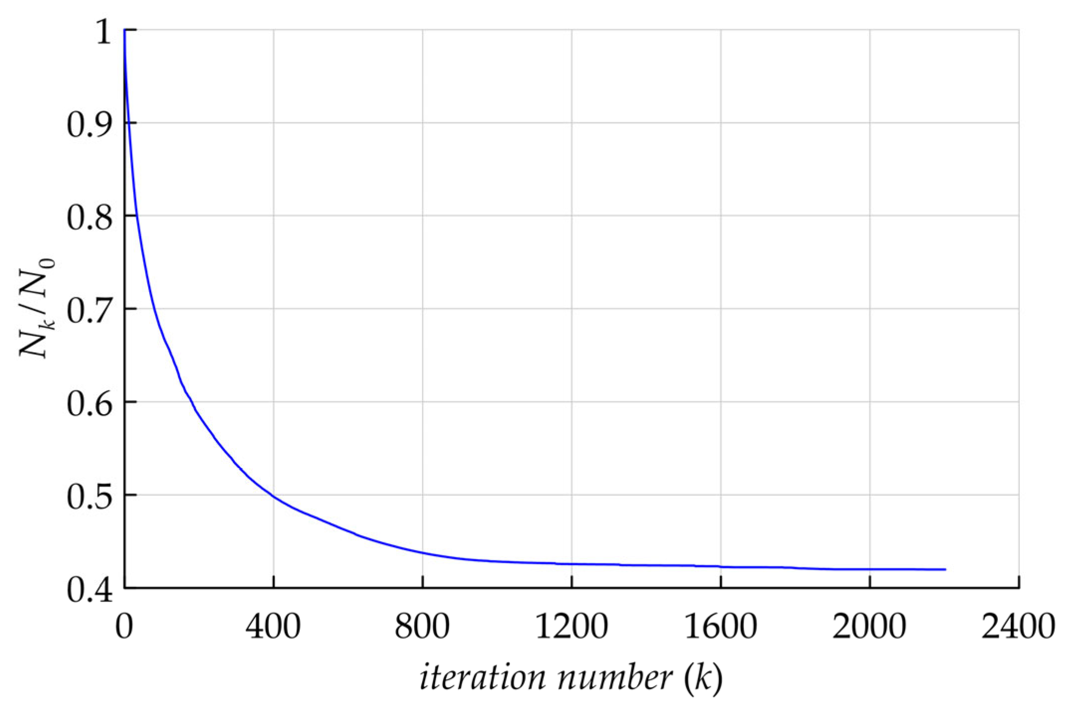
The typical behavior of the iterative process is shown in Figure 2; the difference norm (8) dependence is divided by its initial value $N_0$ on the iteration, the number $k$ is shown. Note that the initial value $N_0$ corresponds to the Jakirlić & Maduta model [24].

The process lasted for 2202 iterations. The norm decreased quickly during the first 1000 iterations, and after this point, it kept close to constant despite the ongoing coefficient change. Let us note that a relatively wide choice of coefficients with which the model accuracy is nearly the same could be used for future tuning for different types of flows. The final value of the norm $N_k/N_0$ was 0.42. Modified model coefficients that correspond to the post-calibration state are the following:

$$\begin{array}{cccc}{C}_{11}=2.5,& C_{12}=0.305,& C_F=0.518,& R{e}_{t0}=266,\\ C_{11}^w=1.39,& C_{12}^w=0.185,& C_l=2.53,& C_{fw}=1.95,\\ C_{21}=0.745,& C_{21}^w=0.00141,& C_{\omega 1}=0.266,& C_{\omega 2}=1.03,\\ {\sigma }_R=1.63,& {\sigma }_{\omega }=2.77,& C_{\omega 3}=0.934,& C_{cr2}=4.73.\end{array}$$

More than half of the coefficients experienced a substantial change. The coefficient $C_{12}$, which is used in the slow part of the redistribution term, was decreased by almost 70%; $R{e}_{t0}$, which affects the region where low-Reynolds number corrections are active, had an increase by 77%; $C_{11}^w$ and $C_{12}^w$, which define the amplitude of the near-wall corrections to the slow part of the redistribution term, decreased by 20% and 38% correspondingly. $C_{21}^w$ is close to zero after the calibration, which means that the near-wall correction to the rapid part of the redistribution term is essentially turned off. $C_{\omega 1}$ and $C_{\omega 2}$, which are responsible for the production and destruction of ${\omega }^h$, were reduced by 40% and raised by 29% correspondingly. This imbalance is towards the destruction of ${\omega }^h$ was compensated by a heightened value of the cross-diffusion coefficient $C_{cr2}$, which became 17.2 times that of its initial value. Finally, the coefficients ${\sigma }_R$ and ${\sigma }_{\omega }$, which are inversely proportional to the intensity of the turbulent diffusion of $R_{ij}$ and ${\omega }^h$, noticeably grew by 48% and 2.5 times correspondingly. The change in coefficients during the difference norm $N_k/N_0$ decrease is presented in Figure 3.

The most important coefficients that are the first to change are $C_l$, $R{e}_{t0}$ and $C_{\omega 2}$. After that, $C_{21}^w$, ${\sigma }_R$, $C_{11}^w$, $C_{21}$, $C_{\omega 1}$, $C_{fw}$ and $C_{12}$ join the trend. These ten coefficients are enough to lower the difference norm to 0.48. Only at the end of the calibration process, when the difference norm is lowered to 0.42 $C_{cr2}$, ${\sigma }_{\omega }$, $C_F$, $C_{12}^w$ and $C_{\omega 3}$ start to change. As it turned out, $C_{11}$ did not change during the calibration.

The physical implications of coefficient changes are as follows. First, the dissipation tensor anisotropy contribution to the slow part of the redistribution term seems to be much lower than was suggested in the baseline model. Second, the magnitudes of both parts of the near-wall corrections to the redistribution term appear to be overestimated in the baseline model, too. Most notably, the ${\mathsf{\Phi }}_{ij,2}^w$ the term was nullified during the calibration, indicating its unimportance. Third, the diffusion intensities of $R_{ij}$ and ${\omega }^h$ were reduced, possibly to compensate for the increase in velocity fluctuation magnitudes. Finally, the cross-diffusion term was found to be relevant at the late stages of the calibration. These observations may serve as guidelines for future developments of the near-wall DRSMs.

3. Testing within the RANS Framework

The Jakirlić & Maduta model [24] with baseline and modified sets of coefficients were implemented in an in-house CFD code zFlare [36]. In this program, using the finite-volume method, the complete system of Reynolds equations for a compressible gas is solved with the possibility of RANS/LES hybridization. Multiblock structured grids and an implicit time integration method DIRK22 (Diagonally Implicit Runge–Kutta Method, two stages, 2nd order of accuracy) [37] are used. In RANS simulations, the spatial approximation of convective terms was performed according to the WENO5 scheme (Weighted Essentially Non-Oscillatory, 5th order) [38] along the grid lines. For diffusion and source terms, 2-nd-order-accurate central difference formulas were used. To verify the software implementation of the models, the results of developed channel flow simulations at $R{e}_{\tau }\approx 2000$ using the zFlare program were compared with the results obtained from the auxiliary one-dimensional program calculation. This program was used in the calibration process. The computational grids corresponded to each other. Solutions for both the baseline and the modified models turned out to be practically indistinguishable between the two programs; the relative divergence in the mean velocity and Reynolds stresses profiles were within ${10}^{-3}$. After this verification, the simulations described below were performed.

3.1. Turbulent Channel Flow at Friction Reynolds Number 2000

This subsection considers the developed turbulent channel flow at a Mach number 0.2 calculated by the bulk velocity (nearly incompressible flow). The basic computational grid contained $4\times 65\times 1$ cells, and the wall-adjacent cell height in inner variables was chosen as $y_1^{+}\approx 0.5$. A half of the channel from the wall up to the symmetry plane was modeled. A general view of the grid and boundary conditions is shown in Figure 4. In the coordinate system of the figure, the flow is moving from left to right.

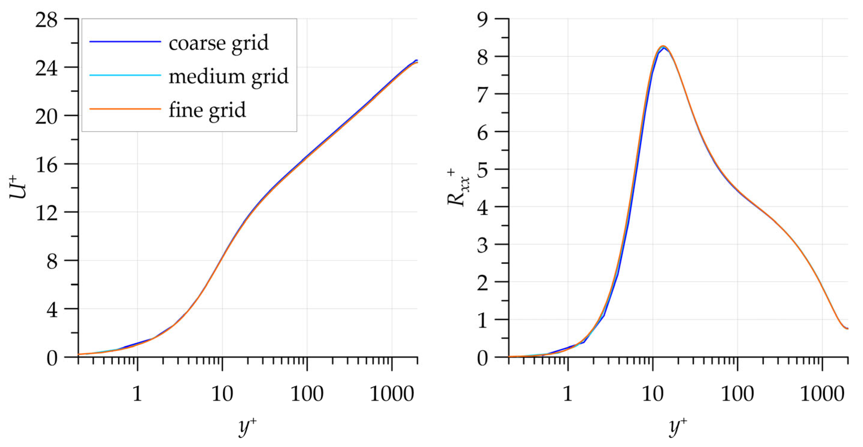
To investigate the grid convergence, nested grids obtained through a consecutive twofold refinement of the base grid in the wall-normal direction were used. In Figure 5, the mean velocity and Reynolds stress $R_{xx}$ profiles obtained on these grids with the modified model are shown. It can be seen that the solutions almost coincide.

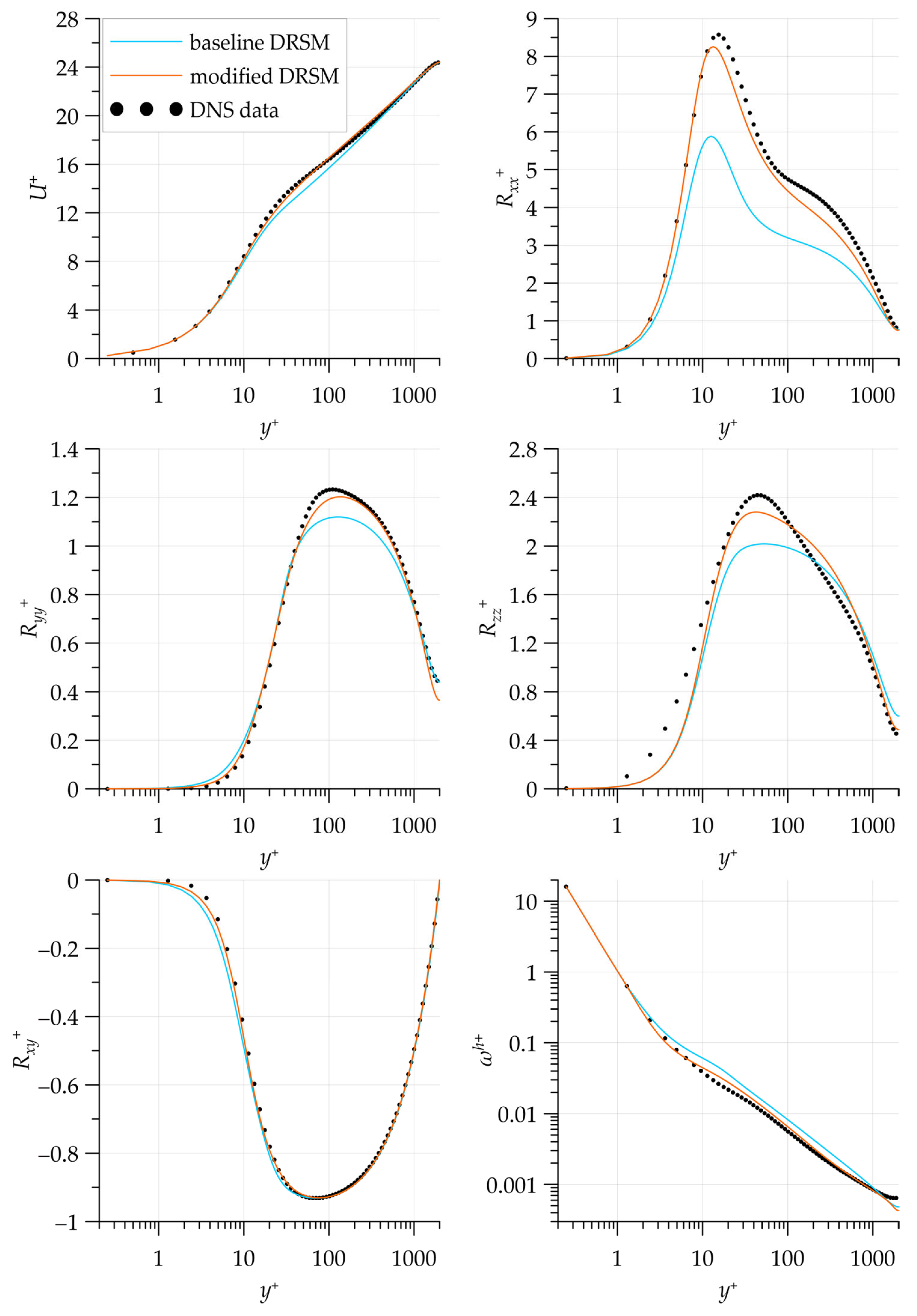
Figure 6 compares the solutions obtained with the baseline and modified versions of the Jakirlić & Maduta model [24] with the DNS reference data [35]. The modified model is close to the DNS data for all the parameters. In particular, the inner peak of the Reynolds stress $R_{xx}$, the behavior of the mean velocity in the buffer region and the distribution of the parameter ${\omega }^h$ across the channel are reproduced significantly better. Noticeable differences from the reference data remain in the $R_{zz}$ profile at $y^{+}<10$. The coefficient recalibration does not affect this distribution. This is caused not by the coefficient values but by the restrictions imposed through the structure of the closures (2), (3), (4). Improving the description of $R_{zz}$ may be an area for a separate study.

3.2. Flat Plate Turbulent Boundary Layer

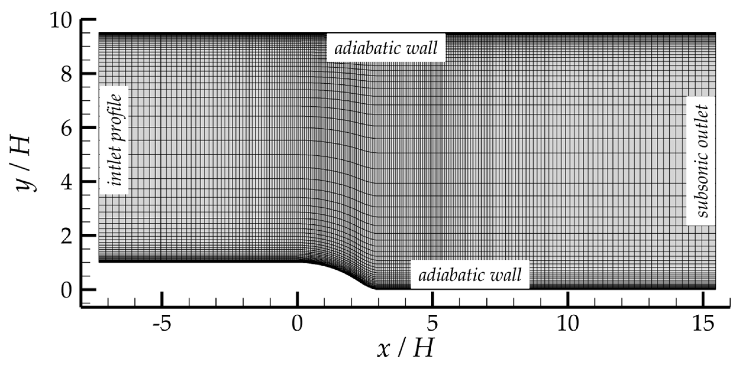
Flat plate turbulent boundary layer simulations were performed in the set-up shown in Figure 7. The length scale $L$ was chosen to be 1 m. The parameters of an inlet flow were prescribed so that the Mach number was equal to 0.2, and the Reynolds number based on $L$ was $5\times {10}^6$. In a preliminary simulation, an extended computational domain was used: the plate leading edge was located at $x=0,$ and a buffer region was placed upstream at $-0.3\le x/L\le 0$. However, it turned out that Jakirlić & Maduta-type models predict a delayed boundary layer transition from a laminar to a turbulent state. To avoid any associated difficulties, an auxiliary simulation using the SSG/LRR-ω DRSM [9] was carried out in the preliminary set-up. In this simulation, almost the entire boundary layer was turbulent. The cross-section $x/L=0.02$ was extracted from this simulation (the Reynolds stress levels there already corresponded to a turbulent flow). The parameters from this section were used as inlet boundary conditions for simulations with the Jakirlić & Maduta models on a “cropped” grid, which had the left boundary located at $x/L=0.02$. This exact computational domain is shown in Figure 7. A subsonic outflow condition with a fixed static pressure was set at the outlet boundary. On the upper boundary, a boundary condition based on the analysis of Riemann invariants was used.

The main grid contained $176\times 384\times 1$ cells. The wall-adjacent cell height in inner variables was within $0.092\le y_1^{+}\le 0.14$ (Figure 8, left, “base grid”). To perform the grid convergence study, simulations were also carried out using the modified model on a grid obtained by removing every second grid line from the original one. It was found that in the interval $0.02\le x/L\le 1.6$, the streamwise distribution of the local momentum-thickness Reynolds number $R{e}_{\theta }$ is reproduced on the two grids within a 1.5% difference. The solutions deviate from each other more noticeably only at $x/L>1.6$ due to the outlet boundary condition influence (Figure 8, right). Note that by definition, $R{e}_{\theta }=U_e{\rho }_e\theta /{\mu }_e$, where $U_e$, ${\rho }_e$, ${\mu }_e$ are the freestream velocity, density, and dynamic viscosity, respectively. Momentum thickness $\theta$ is expressed as

$$\theta ={\int }_0^{\infty }\frac{\rho U}{{\rho }_e{U}_e}\left(1-\frac{U}{U_e}\right)dy.$$

The integration is carried out across the boundary layer in the wall-normal direction.

Consider the wall-normal boundary layer parameter profiles extracted from the control section at $R{e}_{\theta }=6500$ (Figure 9). The DNS results [39] were used as the reference data at the same value of $R{e}_{\theta }$. It can be seen that the modified model improved the velocity distribution compared to the baseline model within the boundary layer. The Reynolds stresses and ${\omega }^h$ parameter distributions also approached the reference data, especially for the inner peak of $R_{xx}$.

It should be noted that at the outer boundary of the turbulent region, the tangent to the velocity profile became almost vertical, accompanied by a local peak of ${\omega }^h$. This may be due to a high value of the cross-diffusion coefficient $C_{cr2}$, which significantly contributes to the solution at boundaries of this type [40]. This occurred because there are no external turbulent region boundaries in the channel flow set-up used for the model calibration. This does not cause an issue since the modified model is supposed to be used as part of hybrid RANS/LES methods. In such simulations, the outer boundaries of turbulent regions are within the LES region and are not affected by the RANS model.

To provide quantitative metrics, the difference norms were calculated using Equation (8) without the summation of the Reynolds numbers. The cross-section corresponding to $R{e}_{\theta }=6500$ was used. The ratio of the modified to the baseline model’s norms was 0.46, close to the channel flow value of 0.42.

Streamwise distributions of the friction coefficient along the plate $C_f=2{\tau }_w/\left({\rho }_e{U}_e^2\right)$, obtained in the simulations and plotted as functions of $R{e}_{\theta }$, are represented in Figure 10. They are compared with the Karman–Schoenherr (KS) empirical correlation [41]:

$$C_f={\left(17.08({\log }_{10}R{e}_{\theta }\right)}^2+25.11({{\log }_{10}R{e}_{\theta })+6.012)}^{-1}.$$

(9)

It can be seen that both the baseline and the modified models reproduce the distribution (9) satisfactorily, and their error level is approximately the same.

3.3. RANS Simulation of a Boundary Layer Separation from a Rounded Step

In this flow, the initially attached boundary layer undergoes separation in the channel expansion region. This test case allows us to evaluate the accuracy of the turbulence model in a flow with a significant streamwise pressure gradient. The choice in favor of the Bentaleb, Lardeau & Leschziner set-up [42] was made due to the simplicity of its geometric formulation and the absence of side walls. The reference data for this flow are the freely available results of a wall-resolved LES simulation [43]. Their reliability is confirmed by considering two computational grids in [42], showing only minor differences in the mean flow fields.

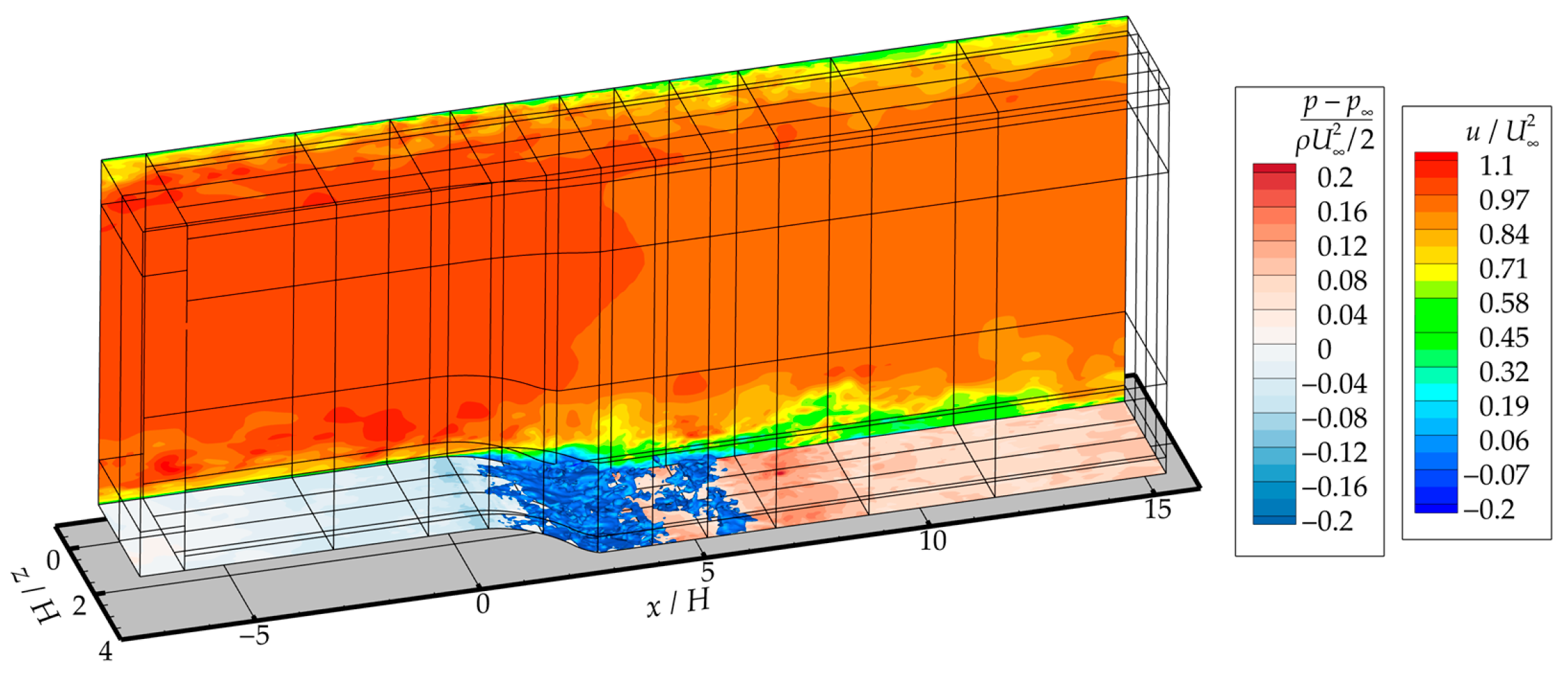
The computational domain consisted of an inlet channel section, an expansion with a rounded backstep and an outlet channel of a constant cross-section, see Figure 11. A flow with the inlet Mach number $M=0.2$ (measured at the channel center) and the Reynolds number $Re={\rho }_{\infty }{U}_{\infty }H/\mu =13,600$ was considered, where ${\rho }_{\infty }$ and $U_{\infty }$ are the density and velocity at the inlet section center, correspondingly, H is a step height and μ is the constant dynamic viscosity. An adiabatic no-slip condition was set on the top and bottom walls, and a constant static pressure was set at the outlet. The solution obtained in a preliminary simulation of the supplying channel was used at the inlet. In that simulation, the velocity and pressure data were taken from the reference LES and did not change during the simulation. The turbulence parameters $R_{ij}$ and ${\omega }^h$ consistent with them were determined.

For the RANS simulations presented here, the grid obtained by modifying the one from the reference LES simulation was used. In the streamwise direction, the original node distribution was left unchanged. In the wall-normal direction, the node distribution of the lower half of the channel was mirrored in the upper half. It was done to use the no-slip condition on the flat (top) wall, whereas wall functions were used in the reference LES simulation. In the spanwise direction, the grid only had one cell due to the statistical spanwise homogeneity of the flow. As a result, the grid consisted of $768\times 252\times 1$ cells.

The grid convergence study showed that coarsening the grid twofold in the $XY$-plane leads to a change in the velocity profiles near the step region within 1% with the considered Jakirlić & Maduta models. This indicates a sufficient grid resolution.

In Figure 12, the profiles of the streamwise and transverse mean velocity components in the expanding channel are shown. It can be seen that in the chosen set-up, the recalibrated model distorts the solution more than the baseline model. The ratio of the modified to the baseline model’s difference norms was calculated using Equation (8). The six cross-sections shown in Figure 12 were used. The ratio was found to be 1.51. This can be explained by the fact that the model was calibrated for flows without adverse pressure gradients in the current study. This seriously limits the applicability of the resulting model in a pure RANS setting. However, as mentioned above, the recalibrated model is intended for use as part of hybrid RANS/LES methods, where its role is limited by a description of the near-wall part of the boundary layer. In this region, the distribution of parameters, such as mean velocity, Reynolds stresses, dissipation rate of turbulence kinetic energy, etc., can be considered close to universal. This allows us to reasonably calibrate the model without using data of flows with a strong streamwise inhomogeneity of the parameters. The following section will demonstrate how the baseline and modified models perform in a hybrid RANS/LES mode in the same test case.

4. Hybrid RANS/LES Simulations of the Curved Step Flow

To demonstrate the recalibrated model performance in the hybrid RANS/LES mode, i.e., in the framework for which it was originally designed, the problem of the boundary layer separation from a curved step was solved again using hybrid methods.

4.1. Formulation of the Hybrid RANS/LES Method Used

In this study, Jakirlić & Maduta type models were hybridized with a recently published differential subgrid stress model [44]. The hybridization was done according to the following formulas:

$$\frac{\partial R_{ij}}{\partial t}+\frac{\partial }{\partial x_k}\left[R_{ij}{U}_k+f_h{T}_{ijk}^{\mathrm{RANS}}+\left(1-f_h\right)T_{ijk}^{\mathrm{LES}}-\frac{\nu }{2}\frac{\partial R_{ij}}{\partial x_k}\right]=P_{ij}+f_h\left({\mathsf{\Phi }}_{ij}^{\mathrm{RANS}}-{\epsilon }_{ij}^{h,\mathrm{RANS}}\right)+(1-f_h)\left({\mathsf{\Phi }}_{ij}^{\mathrm{LES}}-{\epsilon }_{ij}^{\mathrm{LES}}\right),$$

(10)

$$\frac{\partial {\omega }^h}{\partial t}+\frac{\partial }{\partial x_k}\left[{\omega }^h{U}_k-\left(\frac{\nu }{2}+\frac{{\nu }_t}{{\sigma }_{\omega }}\right)\frac{\partial {\omega }^h}{\partial x_k}\right]=f_h{C}_{\omega 1}\frac{{\omega }^h}{k}P-C_{\omega 2}{\left({\omega }^h\right)}^2+\frac{1}{k}{P}_{\omega 3}+S_l+f_h\frac{2}{k}\left(0.55\frac{\nu }{2}+C_{cr2}\frac{{\nu }_t}{{\sigma }_{\omega }}\right)\frac{\partial k}{\partial x_k}\frac{\partial {\omega }^h}{\partial x_k}.$$

(11)

Here $f_h$ is a blending function equal to 1 in the RANS sublayer and to 0 in the LES region. Its formulation is based on the $f_b$ function of the IDDES method [28] and reads as follows:

$$f_h=\min \left\{2\exp \left(-9{\left[0.25-C_{\alpha }\frac{d_w}{{\Delta }_{\max }}\right]}^2\right), 1.0\right\},$$

(12)

where ${\Delta }_{\max }$ is the length of the longest cell edge. Compared to the function of the IDDES method, a coefficient $C_{\alpha }=0.5$ is introduced for increasing the RANS sublayer thickness to a value of about $0.1\delta$ in the boundary layer upstream of the step.

In the Reynolds stress Equation (10), the tensors $T_{ijk}^{\mathrm{RANS}}$, ${\mathsf{\Phi }}_{ij}^{\mathrm{RANS}}$ and ${\epsilon }_{ij}^{h,\mathrm{RANS}}$ are calculated according to the Formulas (2), (3) and (4), respectively. The closures for the tensors $T_{ijk}^{\mathrm{LES}}$, ${\mathsf{\Phi }}_{ij}^{\mathrm{LES}}$ and ${\epsilon }_{ij}^{,\mathrm{LES}}$ are given in Appendix B and correspond to the subgrid stress model [44] with one of the corrections proposed in [45]. In this model, the parameter ${\omega }^h$ is not used. To avoid numerical issues associated with solving the equation for ${\omega }^h$ in the LES region, the production term of ${\omega }^h$, as well as the cross-diffusion term, are multiplied by $f_h$, i.e., are disabled outside the RANS sublayer.

4.2. Setup of the Hybrid Simulations and the Results

The grid for hybrid RANS/LES simulations was obtained by extruding the RANS grid described in Section 3.3 in $z$-axis direction by 96 cells, with the total width of the computational domain in this direction equal to $3.17H$, and by coarsening the grid twofold in the XY-plane. On the side planes, a periodic boundary condition was specified. At the inlet boundary, unsteady disturbances were superimposed on the profiles of the flow parameters according to the method [46], which quickly switched the simulation to the scale-resolving mode. In contrast to RANS simulations, spatial approximation of the convective fluxes was done using the hybrid scheme, which blends the upwind WENO5 approximation in the RANS sublayer and the 2-nd order central differences in the LES region using the formula proposed in [47]. The time step was equal to $0.01t_{char}$, where $t_{char}=H/U_{\infty }$ is the characteristic time of the flow. The period of flow settling was chosen to be equal to $52t_{char}$, after which the solution was averaged over a period of time $270t_{char}$. For illustration, an instantaneous flow field is shown in Figure 13, which was obtained in the hybrid simulation with the recalibrated Jakirlić & Maduta model in the RANS sublayer. It can be seen that an isolated separation is formed near the channel expansion region.

Figure 14 shows the profiles of streamwise and transverse mean velocity components obtained in the hybrid simulations. It is seen that, in contrast to the pure RANS setting, switching to the modified model reduced the size of the separation region to the reference value and caused almost complete agreement with the reference data on the streamwise velocity component. Only minor differences remained visible in the field of the transverse velocity component.

In Figure 15, the components of the Reynolds stress tensor obtained by summing up the resolved and subgrid stresses are compared. One can note an overall overestimation of the stress level by both methods, which is associated either with the features of the subgrid stress model requiring recalibration for shear flows or with an overestimated fluctuation amplitude introduced by the synthetic turbulence generator at the inlet. Note that the modified method captures the position of stress peaks and profile shapes more accurately despite this.

Interestingly, the ratio of the modified to the baseline model’s difference norms calculated using Equation (8) over the six cross-sections shown in Figure 14 and Figure 15 was 0.95. This indicates no significant superiority of the modified model over the baseline. However, this result is attributed to the large discrepancies in the Reynolds stress components, see Figure 15. Calculating the difference norms using only the mean velocity component $U$, a much better ratio is recovered, namely 0.21, consistent with Figure 14. Improving the prediction of the Reynolds stress components in this flow type is the subject of a future study.

Finally, in Figure 16, the streamwise distribution of the pressure coefficient $C_p=(\overline{p}-p_{\infty })/\left(\rho U_{\infty }^2/2\right)$ is shown, where $\overline{p}$ is the mean pressure, $p_{\infty }$ is the pressure at the center of the inlet section, as well as the streamwise distribution of the friction coefficient $C_f$. It can be seen from the $C_p$ distribution that the modified hybrid method captures the drops in the vicinity of the step more accurately. The friction distribution reveals the problem of the synthetic turbulence generator, due to which it is significantly underestimated in the $x<0$ region. However, in the separation region and downstream of it, the friction coefficient is recovered, and its level is reproduced satisfactorily, especially with the modified model.

5. Conclusions

The low-Reynolds-number model of Jakirlić & Maduta [24] was recalibrated using an a posteriori procedure based on DNS data on developed channel flow at Reynolds numbers $R{e}_{\tau }$ in the range of 550–5200. The purpose of the calibration was to obtain a model focused on the description of the thin near-wall part of the boundary layer within the framework of hybrid RANS/LES methods. During the calibration process, the model error was reduced by 58%, which manifested in a better description of the mean velocity profile and the inner Reynolds stress peak and a more accurate distribution of the characteristic turbulence frequency ${\omega }^h$ in the developed channel flow compared to the base model. In the course of the study, an improved wall boundary condition for ${\omega }^h$ was proposed, which was used in all the presented simulations.

Validation of the model within the RANS framework showed that in a zero-pressure gradient flow—a turbulent boundary layer on a flat plate—the modified model gives the same improvement in the description of the flow field compared to the base model as in the developed channel flow. A minor inconsistency was found only at the outer boundary of the boundary layer. This is not a problem since the model is focused on hybrid simulations in which this boundary is located in the LES region. In the RANS simulation of the boundary layer separation from a smooth surface, the modified model showed deterioration in the region of the recirculation zone, which can be explained by the absence of data on flows under adverse pressure gradients in the calibration set. However, in the hybrid RANS/LES simulations, the transition from the base model to the modified one, on the contrary, significantly improved the solution, giving an almost complete coincidence of the mean streamwise velocity with the reference LES data. Thus, the applicability of the modified model to accurately describe the near-wall part of the boundary layer has been confirmed. At the same time, the presented results highlight the importance of the contribution of the RANS model to the overall accuracy of a hybrid simulation.

References

1. Chou, P.Y. On the velocity correlations and the solution of the equations of turbulent fluctuation. Quart. Appl. Math. 1945, 3, 38–54. [Google Scholar] [CrossRef]
2. Rotta, J. Statistische Theorie nichthomogener Turbulenz. Z. Phys. 1951, 129, 547–572. [Google Scholar] [CrossRef]
3. Eisfeld, B. (Ed.) Differential Reynolds Stress Modeling for Separating Flows in Industrial Aerodynamics; Springer: Cham, Switzerland, 2015; 101p. [Google Scholar] [CrossRef]
4. Hanjalić, K.; Launder, B. Modelling Turbulence in Engineering and the Environment. Rational Alternative Routes to Closure, 2nd ed.; Cambridge University Press: Cambridge, UK, 2022; 572p. [Google Scholar] [CrossRef]
5. Hanjalic, K.; Launder, B.E. A Reynolds stress model of turbulence and its application to thin shear flows. J. Fluid Mech. 1972, 52, 609–638. [Google Scholar] [CrossRef]
6. Launder, B.E.; Reece, G.; Rodi, W. Progress in the development of a Reynolds stress turbulence closure. J. Fluid Mech. 1975, 68, 537–566. [Google Scholar] [CrossRef]
7. Lumley, J.L. Computational modeling of turbulent flows. Adv. Appl. Mech. 1979, 18, 123–176. [Google Scholar] [CrossRef]
8. Speziale, C.G.; Sarkar, S.; Gatski, T.B. Modelling the pressure-strain correlation of turbulence: An invariant dynamical systems approach. J. Fluid Mech. 1991, 227, 245–272. [Google Scholar] [CrossRef]
9. Cecora, R.-D.; Radespiel, R.; Eisfeld, B.; Probst, A. Differential Reynolds-Stress Modeling for Aeronautics. AIAA J. 2015, 53, 739–755. [Google Scholar] [CrossRef]
10. Eisfeld, B.; Rumsey, C.L. Length-Scale Correction for Reynolds-Stress Modeling. AIAA J. 2020, 58, 1518–1528. [Google Scholar] [CrossRef]
11. Menter, F.R. Review of the shear-stress transport turbulence model experience from an industrial perspective. Int. J. Comput. Fluid Dyn. 2009, 23, 305–316. [Google Scholar] [CrossRef]
12. Eisfeld, B.; Rumsey, C.; Togiti, V. Verification and validation of a second-moment-closure model. AIAA J. 2016, 54, 1524–1541. [Google Scholar] [CrossRef]
13. Gibson, M.M.; Launder, B.E. Ground effects on pressure fluctuations in the atmospheric boundary layer. J. Fluid Mech. 1978, 86, 491–511. [Google Scholar] [CrossRef]
14. Craft, T.J.; Launder, B.E. New wall-reflection model applied to the turbulent impinging jet. AIAA J. 1992, 30, 2970–2972. [Google Scholar] [CrossRef]
15. Launder, B.E.; Li, S.-P. On the elimination of wall-topography parameters from second-moment closure. Phys. Fluids 1994, 6, 999–1006. [Google Scholar] [CrossRef]
16. Craft, T.J.; Launder, B.E. A Reynolds stress closure designed for complex geometries. Int. J. Heat Fluid Flow 1996, 17, 245–254. [Google Scholar] [CrossRef]
17. Craft, T.J. Developments in a low-Reynolds-number second-moment closure and its application to separating and reattaching flows. Int. J. Heat Fluid Flow 1998, 19, 541–548. [Google Scholar] [CrossRef]
18. Hanjalić, K.; Jakirlić, S.; Hadžić, I. Expanding the limits of “equilibrium” second-moment turbulence closures. Fluid Dyn. Res. 1997, 20, 25–41. [Google Scholar] [CrossRef]
19. Hanjalić, K.; Jakirlić, S. Contribution towards the second-moment closure modelling of separating turbulent flows. Comp. Fluids 1998, 27, 137–156. [Google Scholar] [CrossRef]
20. Jakirlic, S.; Hanjalic, K. A new approach to modelling near-wall turbulence energy and stress dissipation. J. Fluid Mech. 2002, 539, 139–166. [Google Scholar] [CrossRef]
21. Probst, A.; Radespiel, R. Implementation and Extension of a Near-Wall Reynolds-Stress Model for Application to Aerodynamic Flows on Unstructured Meshes. In Proceedings of the 46th AIAA Aerospace Sciences Meeting and Exhibit, Reno, NV, USA, 7–10 January 2008. [Google Scholar] [CrossRef]
22. Cécora, R.D.; Radespiel, R.; Jakirlić, S. Modeling of Reynolds-stress augmentation in shear layers with strongly curved velocity profiles. In Differential Reynolds Stress Modeling for Separating Flows in Industrial Aerodynamics; Eisfeld, B., Ed.; Springer: Cham, Switzerland, 2015; pp. 85–101. [Google Scholar] [CrossRef]
23. Morsbach, C. Reynolds Stress Modelling for Turbomachinery Flow Applications. Ph.D. Thesis, TU Darmstadt, Darmstadt, German, 2016. [Google Scholar]
24. Jakirlić, S.; Maduta, R. Extending the bounds of ‘steady’ RANS closures: Toward an instability-sensitive Reynolds stress model. Int. J. Heat Fluid Flow 2015, 51, 175–194. [Google Scholar] [CrossRef]
25. Gerolymos, G.A.; Vallet, I. Wall-normal-free Reynolds-stress closure for three-dimensional compressible separated flows. AIAA J. 2001, 39, 1833–1842. [Google Scholar] [CrossRef]
26. Gerolymos, G.A.; Sauret, E.; Vallet, I. Contribution to single-point closure Reynolds-stress modelling of inhomogeneous flow. Theor. Comput. Fluid Dyn. 2004, 17, 407–431. [Google Scholar] [CrossRef]
27. Gerolymos, G.A.; Lo, C.; Vallet, I.; Younis, B.A. Term-by-term analysis of near-wall second moment closures. AIAA J. 2012, 50, 2848–2864. [Google Scholar] [CrossRef]
28. Shur, M.L.; Spalart, P.R.; Strelets, M.K.; Travin, A.K. A hybrid RANS-LES approach with delayed-DES and wall-modelled LES capabilities. Int. J. Heat Fluid Flow 2008, 29, 1638–1649. [Google Scholar] [CrossRef]
29. Devenport, W.J.; Lowe, K.T. Equilibrium and non-equilibrium turbulent boundary layers. Prog. Aerosp. Sci. 2022, 131, 100807. [Google Scholar] [CrossRef]
30. Girimaji, S.S. Partially-averaged Navier–Stokes model for turbulence: A Reynolds-averaged Navier–Stokes to direct numerical simulation bridging method. J. Appl. Mech. 2006, 73, 413–421. [Google Scholar] [CrossRef]
31. Chaouat, B.; Schiestel, R. A new partially integrated transport model for subgrid-scale stresses and dissipation rate for turbulent developing flows. Phys. Fluids 2005, 17, 065106. [Google Scholar] [CrossRef]
32. Menter, F. Stress-blended eddy simulation (SBES)—A new paradigm in hybrid RANS-LES modeling. In Proceedings of the Sixth HRLM Symposium, Strasbourg University, Strasbourg, France, 26–28 September 2016; Available online: https://hrlm6.sciencesconf.org/118745/Menter_Abstract.pdf (accessed on 30 August 2023).
33. Jakirlić, S.; Jovanović, J. On unified boundary conditions for improved predictions of near-wall turbulence. J. Fluid Mech. 2010, 656, 530–539. [Google Scholar] [CrossRef]
34. Wilcox, D.C. Turbulence Modeling for CFD, 3rd ed.; DCW Industries: La Cañada, CA, USA, 2006; 522p. [Google Scholar]
35. Lee, M.; Moser, R.D. Direct numerical simulation of turbulent channel flow up to Reτ ≈ 5200. J. Fluid Mech. 2015, 774, 395–415. [Google Scholar] [CrossRef]
36. Troshin, A.; Bakhne, S.; Sabelnikov, V. Numerical and physical aspects of large-eddy simulation of turbulent mixing in a helium-air supersonic co-flowing jet. In Progress in Turbulence IX; Örlü, R., Talamelli, A., Peinke, J., Oberlack, M., Eds.; Springer: Berlin/Heidelberg, Germany, 2021; pp. 297–302. [Google Scholar] [CrossRef]
37. Alexander, R. Diagonally Implicit Runge-Kutta Methods for Stiff O.D.E.’s. SIAM J. Numer. Anal. 1977, 14, 1006–1021. [Google Scholar] [CrossRef]
38. Jiang, G.-S.; Shu, C.-W. Efficient Implementation of Weighted ENO Schemes. J. Comput. Phys. 1996, 126, 202–228. [Google Scholar] [CrossRef]
39. Available online: https://torroja.dmt.upm.es/turbdata/blayers/high_re/profiles/ (accessed on 15 August 2023).
40. Kok, J.C. Resolving the Dependence on Freestream Values for the k-ω Turbulence Model. AIAA J. 2000, 38, 1292–1295. [Google Scholar] [CrossRef]
41. Schoenherr, K.E. Resistances of flat surfaces moving through a fluid. Trans. SNAME 1932, 40, 279–313. [Google Scholar]
42. Bentaleb, Y.; Lardeau, S.; Leschziner, M.A. Large-eddy simulation of turbulent boundary layer separation from a rounded step. J. Turbul. 2012, 13, N4. [Google Scholar] [CrossRef]
43. Available online: https://turbmodels.larc.nasa.gov/Other_LES_Data/curvedstep.html (accessed on 15 August 2023).
44. Balabanov, R.; Usov, L.; Troshin, A.; Vlasenko, V.; Sabelnikov, V. A Differential Subgrid Stress Model and Its Assessment in Large Eddy Simulations of Non-Premixed Turbulent Combustion. Appl. Sci. 2022, 12, 8491. [Google Scholar] [CrossRef]
45. Balabanov, R.; Usov, L.; Nozdrachev, A.; Troshin, A.; Vlasenko, V.; Sabelnikov, V. Assessment of a Differential Subgrid Stress Model for Large-Eddy Simulations of Turbulent Unconfined Swirling Flames. Fire 2023, 6, 94. [Google Scholar] [CrossRef]
46. Shur, M.L.; Spalart, P.R.; Strelets, M.K.; Travin, A.K. Synthetic Turbulence Generators for RANS-LES Interfaces in Zonal Simulations of Aerodynamic and Aeroacoustic Problems. Flow Turbul. Combust. 2014, 93, 63–92. [Google Scholar] [CrossRef]
47. Guseva, E.K.; Garbaruk, A.V.; Strelets, M.K. An automatic hybrid numerical scheme for global RANS-LES approaches. In Proceedings of the International Conference PhysicA.SPb/2016, Saint Petersburg, Russia, 1–3 November 2016. [Google Scholar] [CrossRef]
Figure 1. Near-wall ω h + distributions extracted from the channel flow DNS data [35] and their approximation. ω h + is multiplied by y + 2 for convenience.
Energies 16 06826 g001
Figure 2. The behavior of the difference norm during the iteration process.
Energies 16 06826 g002
Figure 3. The behavior of the coefficients during the difference norm decrease. All coefficients are divided by their initial values, which is denoted by a star.
Energies 16 06826 g003
Figure 4. A computational grid used to simulate the turbulent channel flow and the boundary conditions.
Energies 16 06826 g004
Figure 5. Grid convergence study in the turbulent channel flow test case.
Energies 16 06826 g005
Figure 6. Turbulent channel flow solutions.
Energies 16 06826 g006
Figure 7. Computational grid used to simulate the flat plate turbulent boundary layer and the boundary conditions. Every 4-th grid line is shown.
Energies 16 06826 g007
Figure 8. Dimensionless wall-adjacent cell height (left) and R e θ distributions along the plate (right).
Energies 16 06826 g008
Figure 9. Flat plate turbulent boundary layer solutions.
Energies 16 06826 g009
Figure 10. Friction coefficient distribution along the plate.
Energies 16 06826 g010
Figure 11. Computational grid used to simulate the rounded step flow and the boundary conditions. Every 4-th grid line is shown.
Energies 16 06826 g011
Figure 12. Mean streamwise (upper) and transverse (lower) velocity profiles. Baseline DRSM (blue line), modified DRSM (orange line), reference LES (black symbols). Step geometry is shown in grey.
Energies 16 06826 g012
Figure 13. Instantaneous flow field in the curved step flow hybrid simulation. Streamwise velocity (vertical plane), pressure (lower surface) and zero streamwise velocity isosurface.
Energies 16 06826 g013
Figure 14. Mean streamwise (upper) and transverse (lower) velocity profiles. Hybrid simulation with the baseline model in the RANS subregion (blue line) and the modified model in the RANS subregion (orange line). Black symbols correspond to reference LES. Step geometry is shown in grey.
Energies 16 06826 g014
Figure 15. Reynolds stress profiles. Hybrid simulation with the baseline model in the RANS subregion (blue line) and the modified model in the RANS subregion (orange line). Black symbols correspond to reference LES. Step geometry is shown in grey.
Energies 16 06826 g015
Figure 16. Pressure (upper) and friction (lower) coefficient distributions.
Energies 16 06826 g016