Article

Virtual Inertia Implemented by Quasi-Z-Source Power Converter for Distributed Power System

College of Mechatronics and Control Engineering, Shenzhen University, Shenzhen 518060, China
*
Author to whom correspondence should be addressed.
Energies 2023, 16(18), 6667; https://doi.org/10.3390/en16186667
Submission received: 8 August 2023 / Revised: 11 September 2023 / Accepted: 14 September 2023 / Published: 17 September 2023

Abstract

:
This paper proposes a novel virtual inertia control strategy for distributed power systems with high penetration of renewable energy sources. The strategy uses a quasi-Z-source power converter to emulate the inertia response of a synchronous generator by regulating the DC-link capacitor voltage in proportion to the grid frequency deviation. This paper analyzes the effect of inertia on the frequency regulation of a single-area power system and derives the parameter design method and limitations of the virtual inertia. The paper also introduces the working principle and modulation technique of the quasi-Z-source power converter and presents the virtual inertia control scheme based on a voltage-frequency controller. The paper verifies the feasibility and effectiveness of the proposed strategy through MATLAB/Simulink simulations and dSPACE semi-physical experiments. The results show that the proposed strategy can reduce the frequency deviation and rate of change of frequency (RoCoF) by 20% and 50%, respectively, under load disturbances. The paper demonstrates that the quasi-Z-source power converter can provide flexible and adjustable virtual inertia for distributed power systems without additional energy storage devices.

1. Introduction

Renewable energy generation technology is the most widely used and representative energy development direction in the world. Promoting the development and utilization of renewable energy is the trend of energy policies in various regions [1]. As the penetration rate of renewable energy in the grid increases, the inertia of the grid will gradually decrease since renewable energy is integrated into the grid through static power electronic converters that do not contain any inertia. The reduction in inertia will cause the deviation value of the grid to be more significant when the frequency fluctuates and will seriously threaten the stability and reliability of the power system [2,3].
Inertia is an inherent property of the rotor of a Synchronous Generator (SG). The SG rotor automatically slows down and releases the kinetic energy stored in its rotor to reduce the Rate of Change of Frequency (RoCoF) of the grid when the grid frequency drops. Moreover, it also helps to minimize the maximum deviation of frequency dips. The frequency response curve of a synchronous motor in a power system in the event of a network-side tripping event is shown in Figure 1, where only the primary frequency regulation process is given and the secondary frequency regulation process is neglected. The inertia effect mentioned above is also shown in Figure 1, and the load reduction process is similar to it [4].
Recently, different solutions to solve the decreasing inertia problem of distributed power systems have been proposed by a large number of scholars. The mainstream inertia improvement method uses wind turbines to simulate inertia generation. The virtual inertia control strategy in wind power systems, based on energy storage technology, including fuzzy control and state observers to compensate for wind turbine inertia, was studied in [5,6]. Limited torque control was presented in [7] to provide inertia responses, and an energy storage device was used to solve the frequency drop problem of the Doubly Fed Induction Generator (DFIG) in the process of rotor speed recovery. Based on the droop control strategy, [8] proposed to allow wind turbines to participate in a frequency regulation process so that they can continuously provide virtual inertia support for the power system.
The majority of the existing research focuses on alternative methods for enhancing inertia, apart from the utilization of grid-level energy storage technologies like batteries, supercapacitors, and flywheels, which serve to compensate for grid frequency deviations. The photovoltaic storage system’s storage battery device was proposed in [9], and the battery’s charge and discharge rate is adjusted quickly by calculating the grid frequency and battery state to generate virtual inertia. In [10], the frequency nadir, settling frequency, and RoCoF of battery energy-storage systems (BESS) are improved via a flexible synthetic inertial control technique. The grid RoCoF is determined using a frequency-locked loop like a phase-locked loop [11], which directly influences battery output power. In [12], an adaptive inertial simulation control strategy for a high-speed flywheel energy storage system uses a power excitation method to evaluate the disturbance level to engage in frequency regulation quickly and accurately. The authors of [13] propose a virtual inertia control approach for wind power, solar, and energy storage equipment during mild disturbances. Experimental testing has not confirmed this method. Energy storage devices can boost system inertia, but they can also cause low efficiency and safety and cost issues.
A concept known as Virtual Synchronous Generator (VSG) technology, which operates grid-connected inverters as synchronous generators, is another well-known method for improving inertia [14,15,16,17,18]. The purpose of using the VSG control strategy is to give the inverter a role similar to that of a synchronous generator so that the accepted theory of traditional power systems can still be used in modern power systems with high levels of renewable energy penetration. Although it is possible to simply increase the inertia of the system by arbitrarily setting the virtual inertia coefficient of the VSG, this is based on the premise that the VSG can output or absorb infinite high power, which is far from proven. Virtual inertia control based on a synchronous generator model is proposed in [19], which introduces the dynamic equations of a synchronous generator into the inverter, making the inverter show an inertia response similar to that of a synchronous generator. This method can replicate the dynamic characteristics of a synchronous generator, but it requires high computational power and accurate parameter estimation. Virtual inertia control can also be achieved through sliding-mode control [20] or voltage-frequency control [21]. Sliding-mode control forms a sliding-mode surface between output power and the grid frequency of the inverter, effectively suppressing system disturbance and uncertainty. However, it requires a reasonable sliding-mode surface design and gain design. On the other hand, voltage-frequency control makes the DC-side capacitor voltage proportional to the grid frequency, allowing for simple adjustment of the virtual inertia time constant. Still, it requires consideration of the limitation of the DC-side capacitor voltage.
This study presents a novel virtual inertia technique to solve the aforementioned inertia problem. It simulates the grid-required inertia by using the capacitor group on the DC side of the quasi-Z-source grid-connected power converter. The Z-source converter aims to overcome some of the limitations of traditional power electronics converters. The topologies, modulation techniques, and application of Z-source converters were studied in [22,23]. Z-source converters can be classified into two types: Z-source and quasi-Z-source converters. The quasi-Z-source converter has some advantages over the Z-source converter, such as continuous input current, lower voltage stress, and a simpler modulation technique [24]. However, few studies have explored the potential of Z-source converters for providing virtual inertia to distributed power systems, which is the main contribution of this paper.
This work focuses on the utilization of virtual inertia in distributed power systems through the application of quasi-Z-source power converters. It is a novel method that applies Z-source converters to virtual inertia control in distributed power systems, which can enhance the system frequency stability and power quality under various disturbances and uncertainties. The main contributions of the study are:
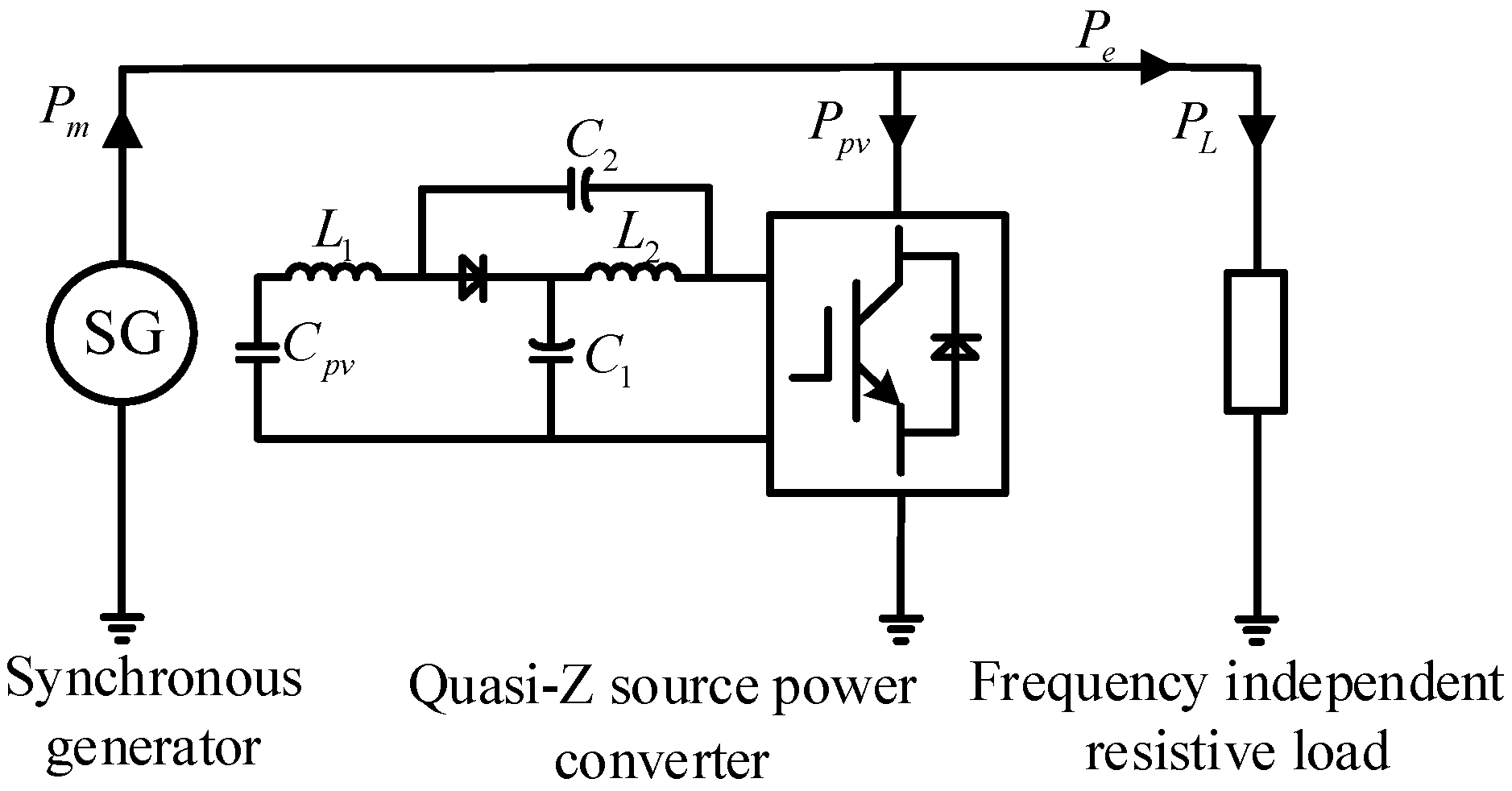
  • Modeling and analyzing a single-area power system with a synchronous generator, a grid-connected power converter, and different types of loads;
  • Developing a virtual synchronous generator control strategy for an inverter to simulate the AC grid and provide grid support;
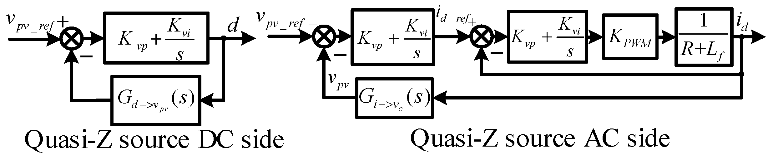
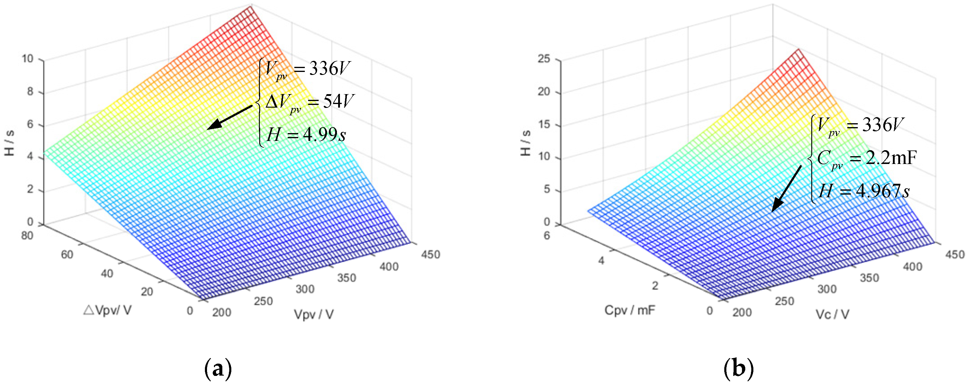
  • Designing a virtual inertia scheme based on the energy stored in the DC-link capacitors of the quasi-Z-source power converter, and deriving the control parameters for the quasi-Z-source side and the AC side;
  • Simulating and experimenting with the proposed virtual inertia control strategy using Matlab/Simulink software and a 1 kW prototype.

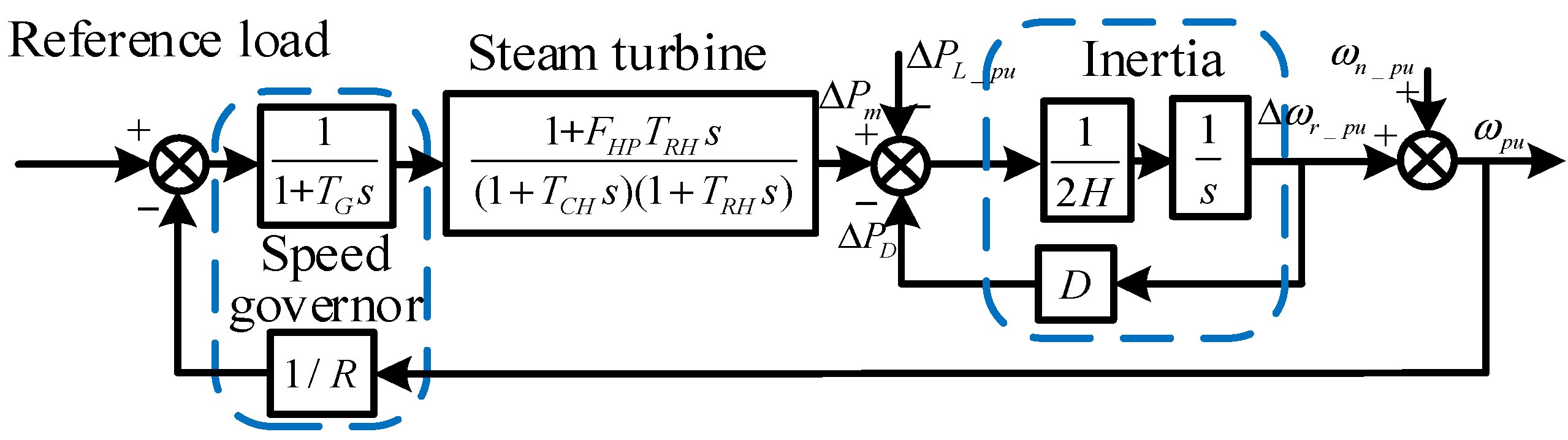
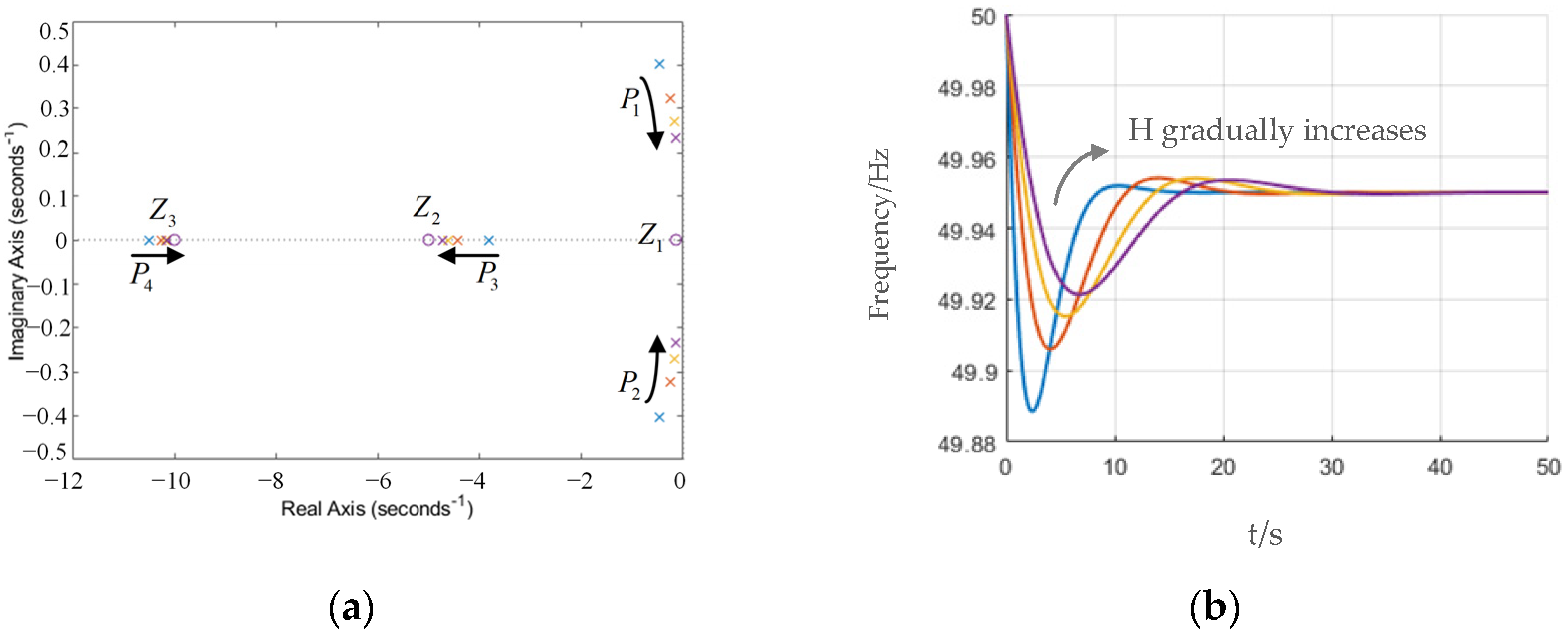
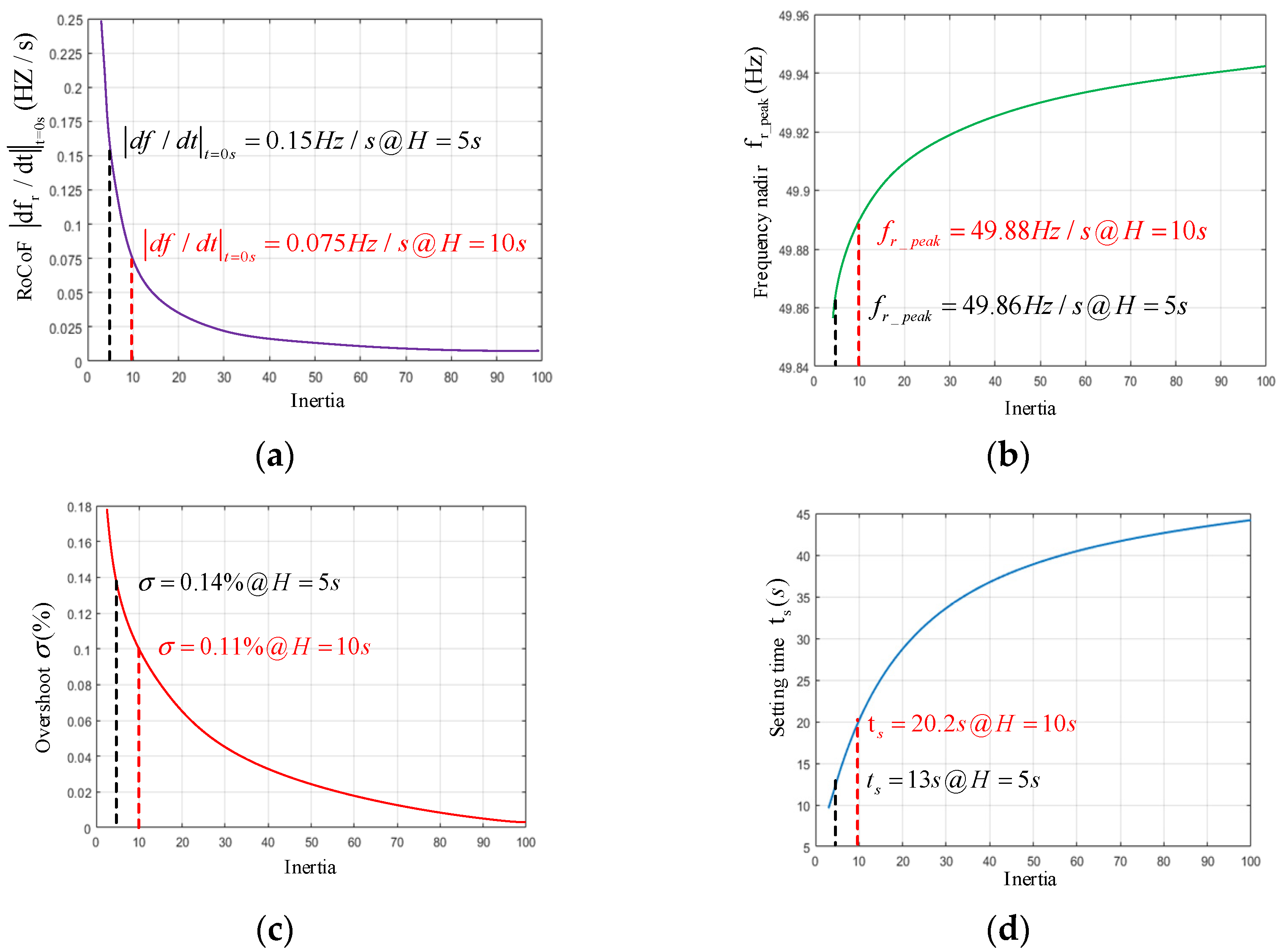
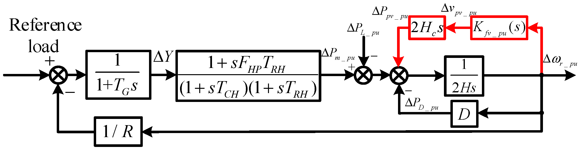
2. Effect of Inertia on Frequency Regulation of Power Systems

A simplified schematic diagram of a single-area power system is shown in Figure 2, which includes several typical components of the power system: a synchronous generator, a renewable energy grid-connected power converter, and a resistive load unaffected by frequency. In this system, Pm is the power generated by the synchronous generator alone, which is provided by the power system to the outside world. Ppv is the difference between the power consumed by the AC/DC rectifier and the power generated by the DC/AC inverter, which is absorbed by the grid-connected power converter. PL is the power consumed by resistive-like loads that are independent of frequency. The grid-side resistive load affects the variability of the output power of the grid-connected power converter. Therefore, Ppv is constant unless there is a load change event in the power system.
It is assumed that the quasi-Z-source grid-connected power converter does not provide virtual inertia support in the single-area power system shown in Figure 2 when the frequency of the power system is regulated by the synchronous generator only. A block diagram of the frequency regulation framework of a typical power system containing a reheat turbine is shown in Figure 3, where TG denotes the time constant of the governor, while FHP, TRH, and TCH are the mechanical time constants of the reheat turbine [25].
Table 1 lists the frequency regulation structure and the associated system parameter values shown in Figure 3. In general, the inertia time constant H is a common measure of the inertia magnitude in power systems. It has typical values of 5 s for gas-fired generators, 3.5 s for coal-fired generators, 3 s for nuclear generators, and 3 s for hydroelectric generators [4]. The well-known second-order Mechanical Oscillation equation, which mathematically describes the electromechanical behavior of synchronous generators, can be derived from Figure 3:
{ Δ P m _ p u Δ P L _ p u = 2 H d Δ ω r _ p u d t + D Δ ω r _ p u H = E g e n / V A r a t e d = J ω r e f 2 / ( 2 V A r a t e d )
where J represents the sum of the moments of inertia of the generator and turbine, H represents the inertia time constant of the synchronous generator at a standardized value, and the relationship with the rotational inertia J is given in (1). Egen represents the rotational kinetic energy of the rotor, and VArated refers to the rated power of the system, which is 1 kW in this paper.
It is worth mentioning that the block diagram of the linearized frequency regulation structure shown in Figure 3 is only applicable to small-signal analysis, where the grid frequency fr fluctuates around its nominal value fref and the frequency regulation performance is not limited by the power rating of the synchronous generator.
To quantify the effect of power system inertia on frequency regulation, the transfer function from load disturbance ΔPm_pu to frequency deviation Δωr_pu can be obtained according to Figure 3 as:
G P L - > ω r = R ( 1 + T G s ) ( 1 + T C H s ) ( 1 + T R H s ) ( 2 H s + 1 ) ( 1 + T G s ) ( 1 + T C H s ) ( 1 + T R H s ) R + F H P T R H s + 1
Figure 4 gives the zero-pole and frequency response plots of (2) under 5% load addition, where the zero point is represented as a circle and the pole as a cross.
The system has a higher-order transfer function (2), which cannot be analyzed using the time-domain performance index of a typical second-order system. However, the figure shows that the system has three zeros and four poles on the real axis, including a pair of conjugate poles. The conjugate poles are the dominant poles, as they are close to the imaginary axis and far from the other poles and zeros. As H increases, the system poles P3 and P4 approach and tend to cancel the zero points Z2 and Z3, which are a pair of dipoles. This reduces the maximum frequency deviation and RoCoF of the system, but also prolongs the regulation time.
Furthermore, (2) is simplified using the dominant pole method; the system is represented by Z1, P1, and P2; and the simplified transfer function obtained is
G P L - > ω r = R ( 1 + T R H s ) ( 2 H s + 1 ) ( T R H s + 1 ) R + F H P T R H s + 1 = G 0 s + Z 1 s 2 + 2 ξ ω n + ω n 2
where ωn and ξ represent the undamped natural frequency and damping ratio, respectively.
By converting (3) into a typical Type II transfer function and combining the parameters listed in Table 1, the relationship between various time-domain performance indicators of the system and the inertia coefficient H can be obtained, as shown in Figure 5; the specific process can be found in [26].
The increase in H will reduce RoCoF|t = 0 s, but increase the frequency peak size, as shown in Figure 5a,b. This shows the effectiveness of the inertia of the power system in suppressing frequency deviation and reducing RoCoF. Nevertheless, a significant load change will cause a more serious RoCoF and the lowest point of the frequency drop. Other methods should be used to prevent such unfavorable load changes. A more considerable H value can attenuate the frequency overshoot, as shown in Figure 5c. However, this will also slow down the dynamic range of the frequency adjustment and prolong the frequency recovery process, as shown in Figure 5d.

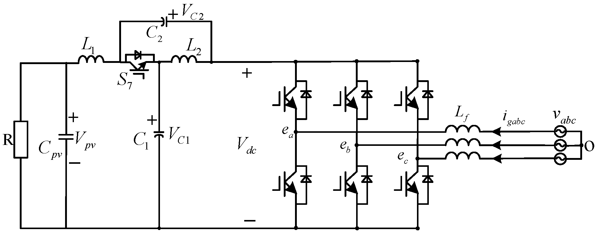
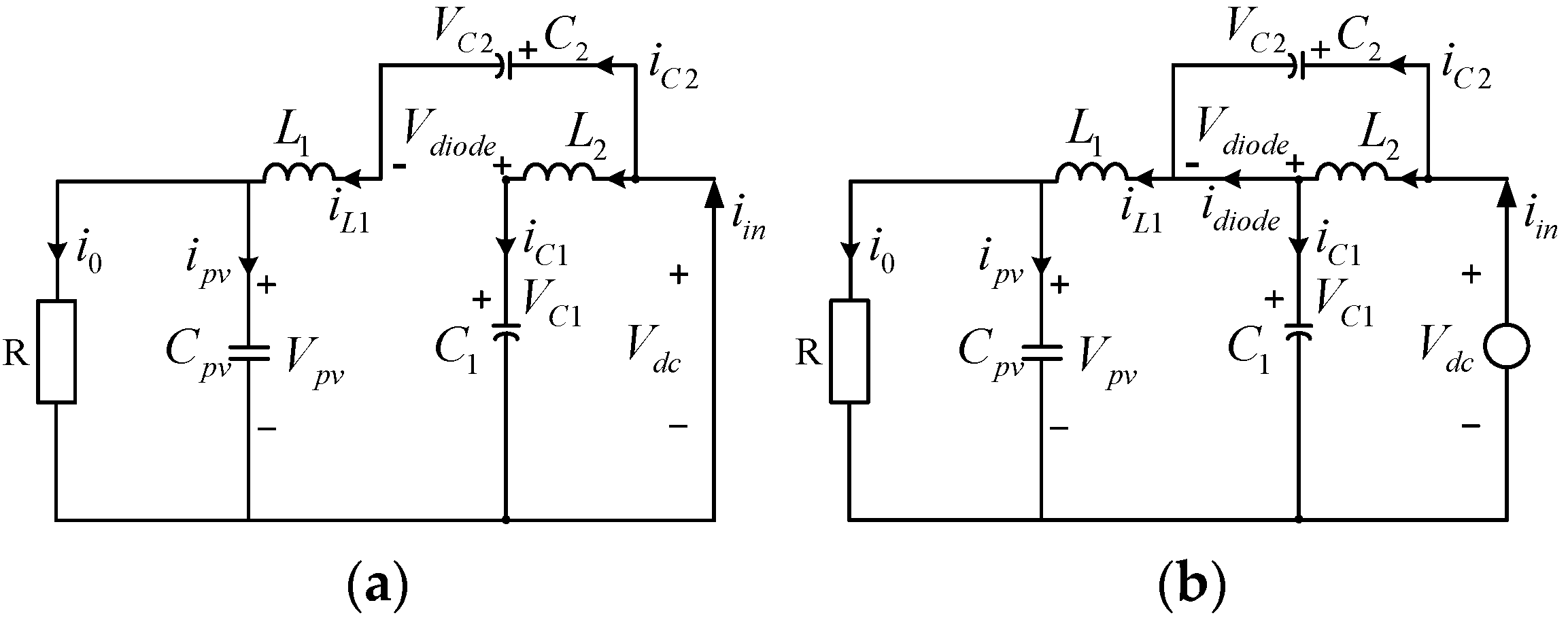
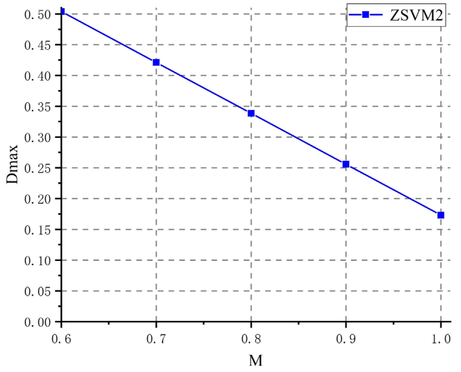
3. Analysis of Quasi-Z-Source Power Converter

The quasi-Z-source circuit is often used in photovoltaic grid-connected applications. In this paper, the quasi-Z-source power converter used to provide virtual inertia is called a Quasi-Z-Source Rectifier (QZSR).
The three-phase QZSR topology diagram is shown in Figure 6. The topology consists of two capacitors, C1 and C2. A filter capacitor, Cpv, with a relatively large capacitance is connected to the DC side to generate virtual inertia. Two inductors, L1 and L2, and a diode, S7, are also included. The diode S7 acts as a switch and needs to be replaced by a switch tube in the QZSR circuit to ensure that it is off in the conducting state and on in the non-conducting state. vabc is the three-phase input voltage of the grid, and Lf is the grid-side filter inductance.
One of the main reasons for selecting the quasi-Z-source rectifier to provide the virtual inertia required by the power system is that the DC-side capacitor bank in the quasi-Z-source circuit can act as an energy storage device that comes with the circuit. Therefore, there is no need to install other redundant energy storage devices to provide energy support. It is called virtual inertia because the simulated inertia provided by the energy stored in the capacitor is different from the inertia of the real synchronous generator, in essence, but they have the same function.
The QZSR circuit operates in two modes: a non-shoot-through state and a shoot-through state. It is assumed that the QZSR has a continuous inductor current, lossless inductance and capacitance of the passive components, and negligible turn-on time loss when analyzing the quasi-Z-source circuit.
The circuit diagram of the two working modes of the QZSR is shown in Figure 7, where Vpv is the output voltage of the DC bus; i0 is the current of the DC bus; VL1, VL2, iL1, and iL2 are the voltage and current of the inductors L1 and L2, respectively; Vc1, Vc2, ic1, and ic2 are the voltage and current of the capacitors C1 and C2, respectively; Vdiode and idiode are the voltage and current of the quasi-Z-source diode, respectively; and the specific reference directions are as shown in the figure.
When the circuit works in the shoot-through state, the switch S7 is turned off by the shutdown signal. The circuit is shown in Figure 7a. The network side is short-circuited and the quasi-Z-source capacitor charges the inductor, so there is
{ V L 1 = V C 2 V p v V L 2 = V C 1 V d c = 0 i C 1 = i L 2 i C 2 = i L 1 i i n = ( i L 1 + i L 2 )
The grid and the quasi-Z-source inductance charge the capacitor and the DC-side load, as shown in Figure 7b, when the circuit works in non-shoot-through states. At this time, the switch tube S7 is turned on. There is:
{ V L 1 = V C 1 V p v V L 2 = V C 2 V d c = V C 1 + V C 2 i C 1 = i i n i L 1 i C 2 = i i n i L 2
Assuming that the quasi-Z-source circuit operates in a steady state in a cycle TS, the duration of the shoot-through state is Tsh, and the duration of the non-shoot-through state, abbreviated as Tnsh, is (TsTsh). The voltage formulas on the inductors L1 and L2 can be obtained based on the circuit volt-second balance principle as follows:
{ V L 1 = v ¯ L 1 = T s h ( V C 2 V p v ) + T n s h ( V C 1 V p v ) T s = 0 V L 2 = v ¯ L 2 = T s h V C 1 + T n s h V C 2 T s = 0
Similarly, the average current on the capacitor during one steady-state cycle is zero, i.e., the circuit expression is:
{ i C 1 = i ¯ C 1 = T s h ( i L 2 ) + T n s h ( i i n i L 1 ) T s = 0 i C 2 = i ¯ C 2 = T s h ( i L 1 ) + T n s h ( i i n i L 2 ) T s = 0
Combining (6) and (7) yields:
{ V C 1 = 1 D 1 2 D V p v V C 2 = D 1 2 D V p v I L 1 = I L 2 = P p v V p v
where D = Tsh/Ts is defined as the duty cycle, while VC1, VC2, Vpv, IL1, IL2, and Vpv refer to the steady-state values of the voltage, current, and power of the respective components in the circuit. According to (6)–(8), the following expressions can be obtained:
{ v ^ d c = V C 1 + V C 2 = 1 1 2 D V p v = B V p v I C 1 = I C 2 = I i n I L , I d i o d e = 2 I L I i n
where BVpv is the peak DC-side bus voltage of the QZSR circuit, B is the boost factor, and Iin is the output DC bus current.

4. Virtual Inertia Control Strategy

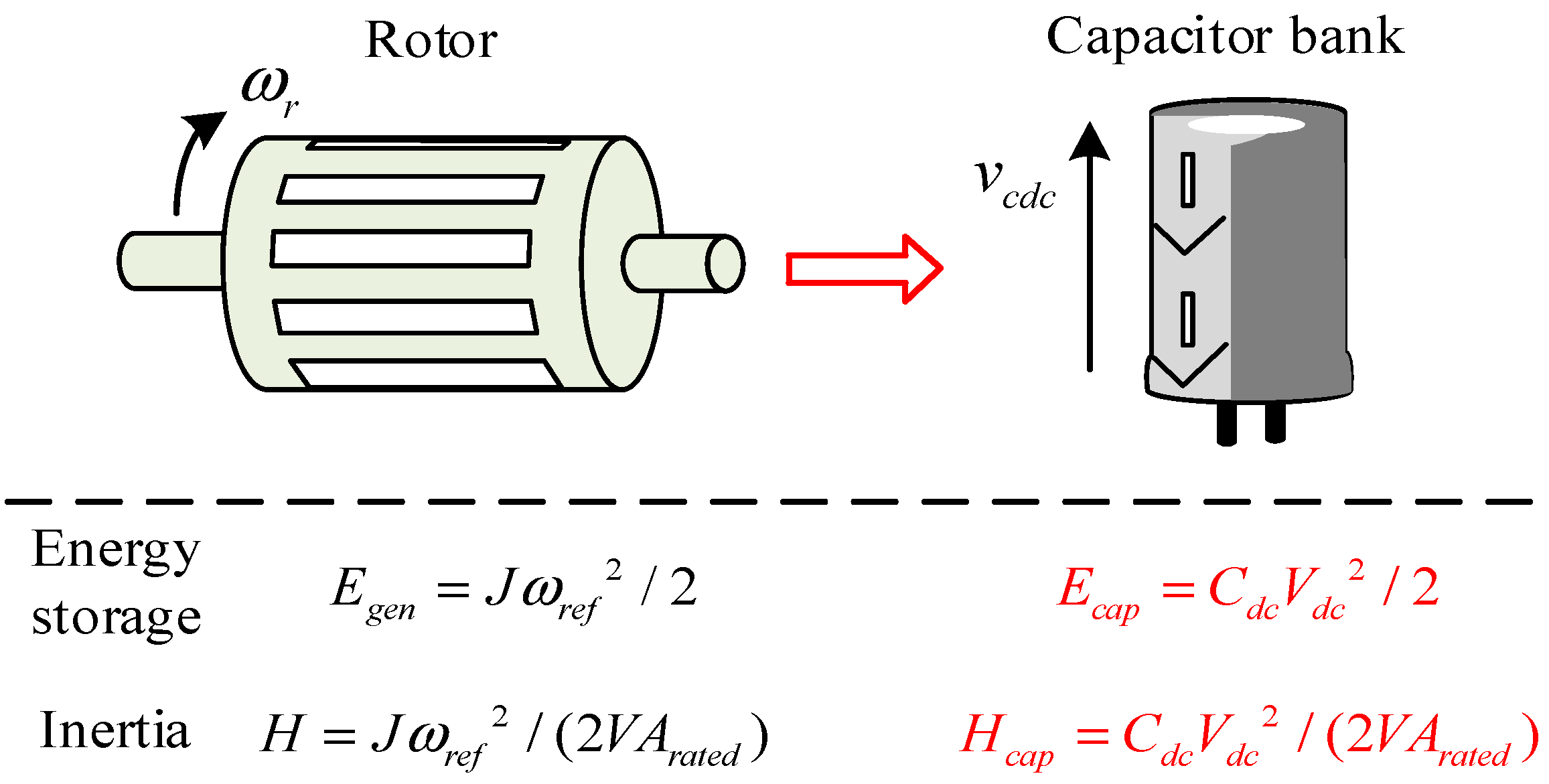
4.1. Mapping of Capacitors to Motor Rotors

A schematic diagram of the inertia mapping between the DC-link capacitor of the quasi-Z-source circuit and the synchronous generator is shown in Figure 8. The rotor mechanical and electrical angular velocities of the synchronous generator with a pair of poles are equal and denoted as ωr, where ωr = 2πfr and fr is the grid frequency. Their respective reference values are indicated as ωref. As shown in Figure 8, the angular frequency ωr and the DC bus voltage vdc play a similar role in determining the respective inertia time constants H and Hcap, which are proportional to the square of ωref and Vcdc_ref, respectively. This observation suggests that if the DC-link capacitor voltage Vcdc_ref is correlated with the grid frequency fr, the DC-link capacitor can release or absorb energy in a similar way to a synchronous generator. Therefore, by using this analogous mapping, the virtual inertia required for a distributed power system can be obtained from a quasi-Z-source grid-connected power converter.
Inertia is the kinetic energy per unit that synchronous generators have in their rotor and turbine. DC-link capacitor banks have an energy storage capacity similar to that of synchronous generators, so the capacitors also have the potential to perform inertia simulation. Based on the previous definition of H, the inertia time factor Hcap of the DC-link capacitor can be defined as
H c a p = E c a p V A b a s e = C c d c V c d c _ r e f 2 2 V A b a s e
where Ccdc and Vcdc_ref denote the DC-link capacitance and DC-link voltage reference values.

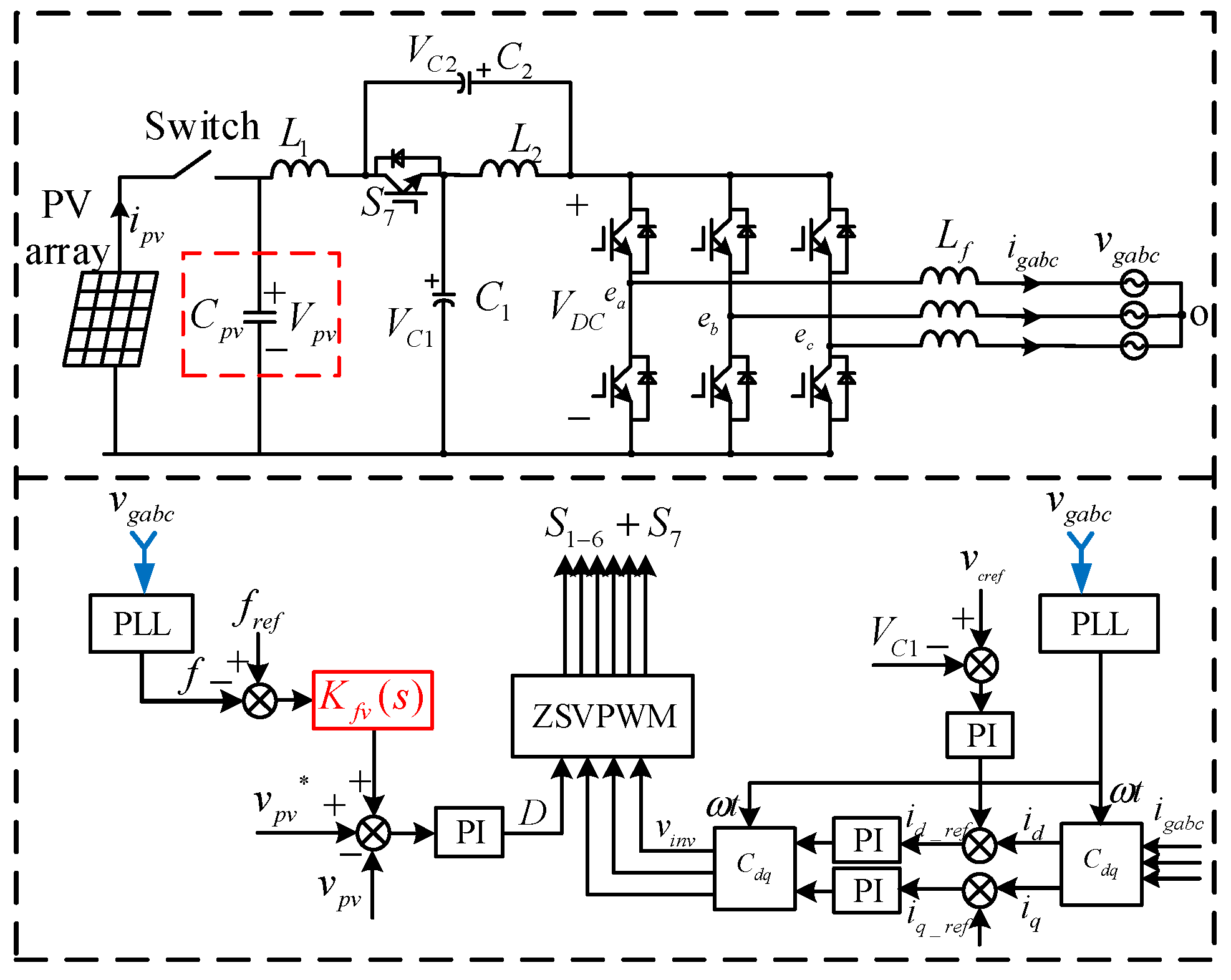
4.2. Quasi-Z-Source Power Converter with Virtual Inertia Strategy

The overall control block diagram of a quasi-Z-source grid-connected power converter with distributed virtual inertia is shown in Figure 9. The inner-loop current controller on the AC side regulates the id and iq in the dq coordinate system based on the reference values id_ref and iq_ref of the grid current. An external voltage loop controller with capacitor C1 stabilizes the inverter input bus voltage, which is the Z-source PWM modulated voltage in the quasi-Z-source topology. This external voltage loop has a similar effect as the DC-side voltage controller of the conventional PWM rectifier. However, due to the special characteristics of the quasi-Z-source topology, the DC-link capacitor voltage on the DC side of the quasi-Z source should also be regulated by a voltage closed-loop controller to generate a shoot-through duty cycle D. The shoot-through ratio and the regulation system of the circuit should be reasonably set to ensure the rectification of the AC side and the voltage conversion on the network side of the quasi-Z source, and not to bring excessive voltage stress to the semiconductor devices in the circuit, causing device damage. The voltage controller on the AC side is implemented as a PI controller, which controls the DC bus voltage Vc1 by changing the value of the d-axis current reference id_ref to track its reference vc1_ref, while the q-axis current reference iq_ref depends on the reactive power requirement of the system for reactive power compensation.
The virtual inertia simulation is generated by the new voltage-frequency controller Kfv(s), shown in Figure 9, which connects the grid frequency change Δf with the DC-link capacitor voltage change Δvpv_ref through the transfer function Kfv(s). When a frequency event occurs in the power system, it changes the DC-link capacitor voltage so that the capacitor can release or absorb energy for inertia simulation. In addition, the control scheme proposed in this paper only uses the DC-link capacitor of the quasi-Z-source power converter without any extra energy storage unit. The DC-link capacitor supports the DC-link voltage and filters harmonics in the grid-connected power converter, so the control scheme does not add any burden to the hardware design. Figure 9 also shows that the PLL detects the grid frequency f from the grid voltage vgabc. Other faster methods for grid frequency detection, such as frequency-locked loop FLL, can also be used in experiments. The PLL dynamic process is ignored in all of the above discussion sections.
When the voltage-frequency controller Kfv(s) is not working, the quasi-Z-source circuit works in the photovoltaic grid-connected state, and the circuit plays the role of transmitting power to the grid. At this point, a block diagram of a conventional three-closed-loop controller can be obtained, as shown in Figure 10. The controller uses a proportional-integral controller for voltage and current control while ignoring the coupling effect between the d-axis and q-axis, which is not drawn in the figure. The magnitude range of the capacitor voltage Vpv used to generate inertia must be limited between [Vpv_min and Vpv_max], where the minimum voltage Vpv_min is to ensure linear modulation of the power converter. The maximum voltage Vpv_max is then determined with the voltage ratings of the active and passive components. The transfer functions Gd related to vpv(s) and Gi related to vc(s) are obtained according to the small-signal model [27].
It is worth mentioning that the ZSVPWM in Figure 9 refers to the quasi-Z-source space vector pulse-width-modulation algorithm, which differs from the conventional PWM modulation algorithm. This paper adopts the ZSVM2 modulation algorithm, which inserts the shoot-through time in any two phases of the three-phase bridge arm and splits each shoot-through time into Tsh/4. This modulation method divides the total required shoot-through time interval into four parts, but only modifies two switching times in the circuit, hence the name ZSVM2 modulation algorithm [28]. When using the ZSVM2 modulation algorithm, the relationship between the circuit modulation ratio M and the shoot-through duty cycle D is crucial for the virtual inertia generated, and the specific limits can be expressed as:
D max = 1 3 3 2 π M
According to the (11), the relationship between the ZSVM2 direct duty cycle and the modulation ratio can be obtained, as shown in Figure 11.
With the proposed voltage-frequency controller applied, the frequency regulation block diagram in Figure 3 changes to Figure 12. In this diagram, Δvpv_pu is passed through the transfer function of 2Hcaps to obtain ΔPpv_pu, and Kfv_pu(s) is the per-unit value of the virtual inertia controller. As a result, the equivalent inertia time-constant shifts H to H + HcapKfv_pu, where the second term can be seen as the virtual inertia constant Hp, given as:
H p = H c K f v _ p u
Since the dynamic response of voltage loop control is much faster than frequency regulation, Kfv_pu (s) can be designed as a proportional controller to generate virtual inertia. The specific expression is:
K f v _ p u = ( Δ V p v _ max V p v ) / ( Δ f r _ max f r e f )
where ΔVpv_max = (Vpv_maxVpv_min)/2 and Δfr_max denote the maximum allowable voltage deviation and frequency deviation, respectively. The system parameters shown in Figure 12 refer to their per-unit value forms, so ΔVpv_max and Δfr_max should be divided by the rated DC-link voltage Vpv and frequency fref. Substituting (10) and (13) into (12), the virtual inertia coefficient Hp can be redefined as:
H p = Δ V p v _ max f r e f V p v Δ f r _ max C p v V p v 2 2 V A r a t e d
Equation (14) shows that the virtual inertia time constant at a given rated power depends on the following factors: DC-link capacitor size Cpv, rated DC-link voltage Vpv, maximum voltage variation rate ΔVpv_max/Vpv, and maximum frequency variation rateΔfr_max/fref.
For a 1 kW quasi-Z-source power converter with a maximum frequency deviation Δfr_max = 0.2 Hz (fref = 50 Hz), the relationship between its virtual inertial time constant Hp and Cpv, Vpv, and ΔVpv_max is shown in Figure 13. The figure indicates that Hp increases with the increases in Cpv, Vpv, and ΔVpv_max. Moreover, the power converter can generate a virtual inertia larger than that of the synchronous generator (the H of different generator sets is usually between 2 s and 10 s). However, this requires a larger Cpv and Vpv, which will increase the capacitance value, DC-link voltage, or voltage deviation, posing challenges to the power converter design in terms of cost, size, and control. Also, the higher ΔVpv_max may limit the overmodulation and shoot-through duty cycle. Therefore, it is advisable to generate only the required inertia for the power system to improve frequency stability.

5. Simulation and Experiment Verification

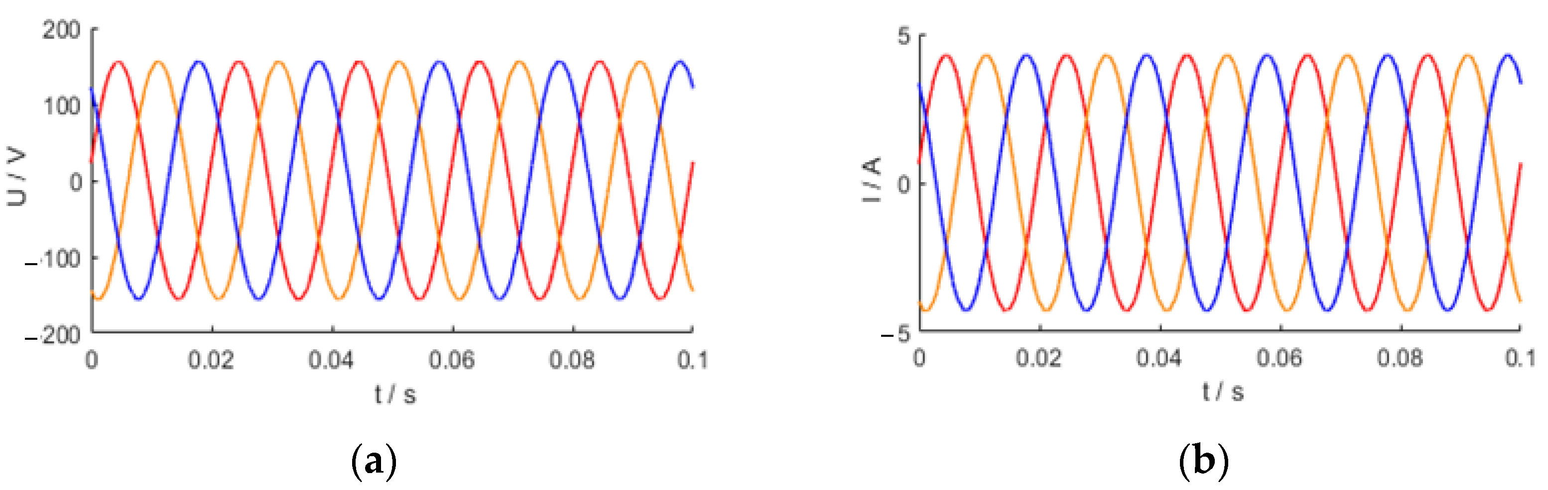
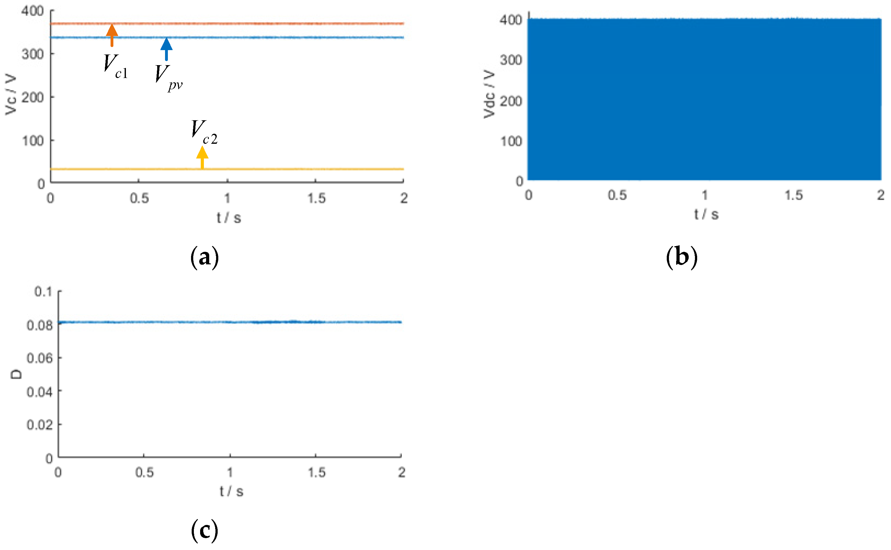
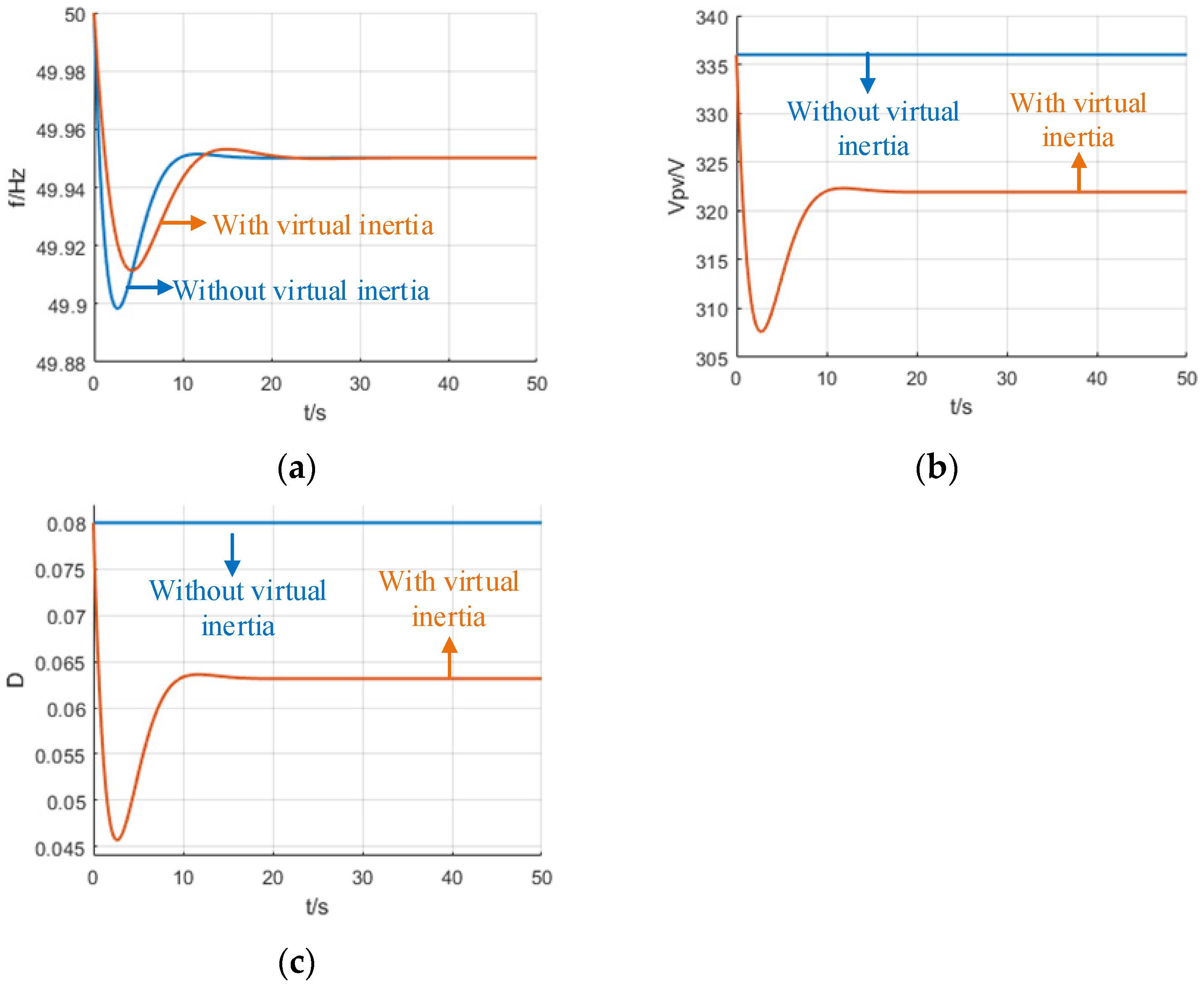
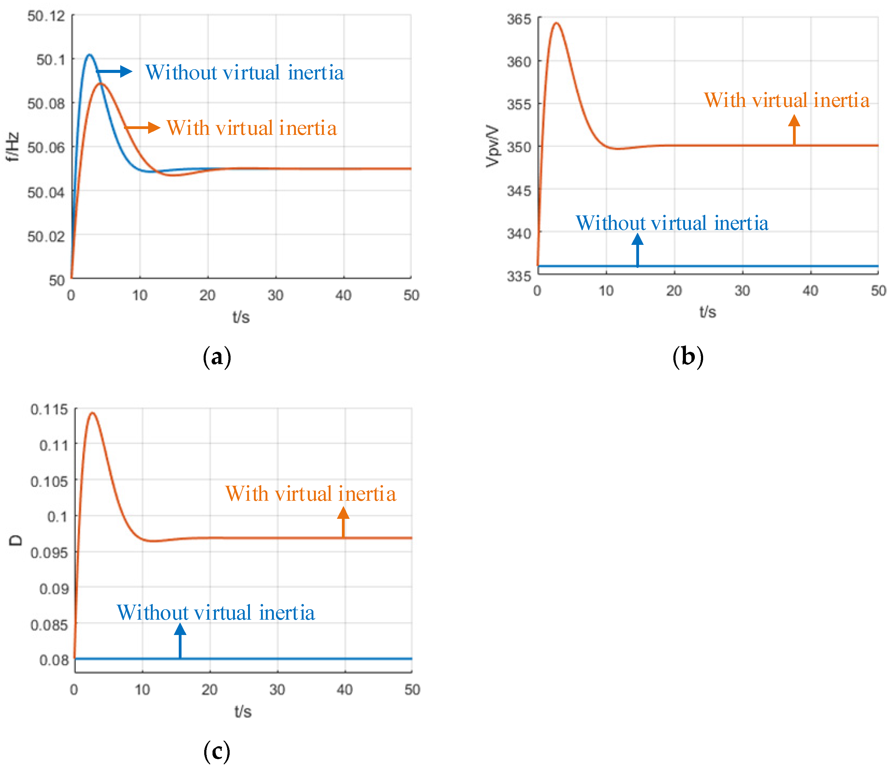
5.1. Simulation Results

The simulation of the proposed virtual inertia control strategy is first built in MATLAB/Simulink. The VSG-controlled inverter and the quasi-Z-source grid-connected power converter circuits were built separately, where the VSG-controlled inverter was used to simulate the AC grid to provide grid frequency support so that the virtual inertia could be reflected.
Some system parameters used in the VSG circuit are as follows: three-phase filter inductance Lf = 0.6 mH and moment of inertia J = 0.1 kg·m2, corresponding to the inertia time of a 1 kW power system. The constant H = 5.0 s and the AC output phase voltage is 110 V; other parameters are given in Table 1. The circuit parameters of the quasi-Z-source power converter are shown in Table 2.
The three-phase output voltage and current of the VSG obtained via simulation are shown in Figure 14, which indicates that the VSG can be used to simulate the AC power grid.
The quasi-Z-source power converter can operate in the grid-connected inverter mode when the proposed voltage-frequency controller Kfv(s) is not working. This mode differs from the QZSR circuit and is called the Quasi-Z-Source Inverter (QZSI) circuit. In this mode, the switch on the DC side is closed, and the photovoltaic array delivers active power to the grid. The output results of the circuit simulation in the inverter mode are shown in Figure 15. Figure 15a shows the quasi-Z-source capacitor voltage C1, C2, and Cpv; Figure 15b shows the input voltage of the QZSI; and Figure 15c shows the shoot-through duty cycle D. In the steady state, the voltages of capacitors C1, C2, and Cpv in the quasi-Z-source circuit and the input voltage to the inverter must satisfy the voltage relationship of the quasi-Z-source circuit when D = 0.08.
The simulation results of the grid frequency response are shown in Figure 16 when the load on the grid side increases by 5% and the voltage-frequency controller is active. Figure 16a shows that the maximum deviation of the grid frequency is about 0.1 Hz without the proposed voltage-frequency controller and about 0.08 Hz with the controller. This means that the proposed virtual inertia method can reduce the frequency deviation by 20%. Moreover, the RoCoF parameter can also be reduced from 0.150 Hz/s to 0.075 Hz/s, which indicates that the power system RoCoF can be decreased by 50% compared with the case without the virtual inertia controller. The proposed voltage-frequency controller allows the power system RoCoF to be determined by both the virtual inertia of the power converter and the power system inertia, and to be flexibly designed according to the virtual inertia coefficient Hp. Figure 16b shows that the quasi-steady-state voltage deviation of the power grid is about 13.5 V, which is proportional to the quasi-steady-state frequency deviation. This voltage deviation is within the maximum allowable voltage deviation of 54 V during frequency events on the grid. Figure 16c shows the variation of the quasi-Z-source direct duty cycle and the modulation ratio M, which satisfies (11).
Similar results can also be observed in Figure 17, but this time, the power system is subjected to a 5% load reduction change on the grid side, and the grid frequency also exceeds 50 Hz during the dynamic adjustment process.

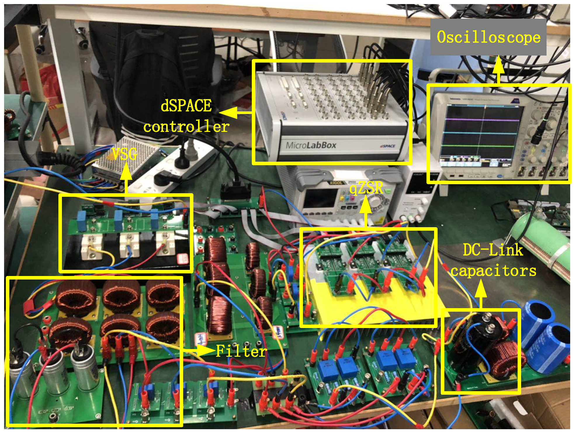
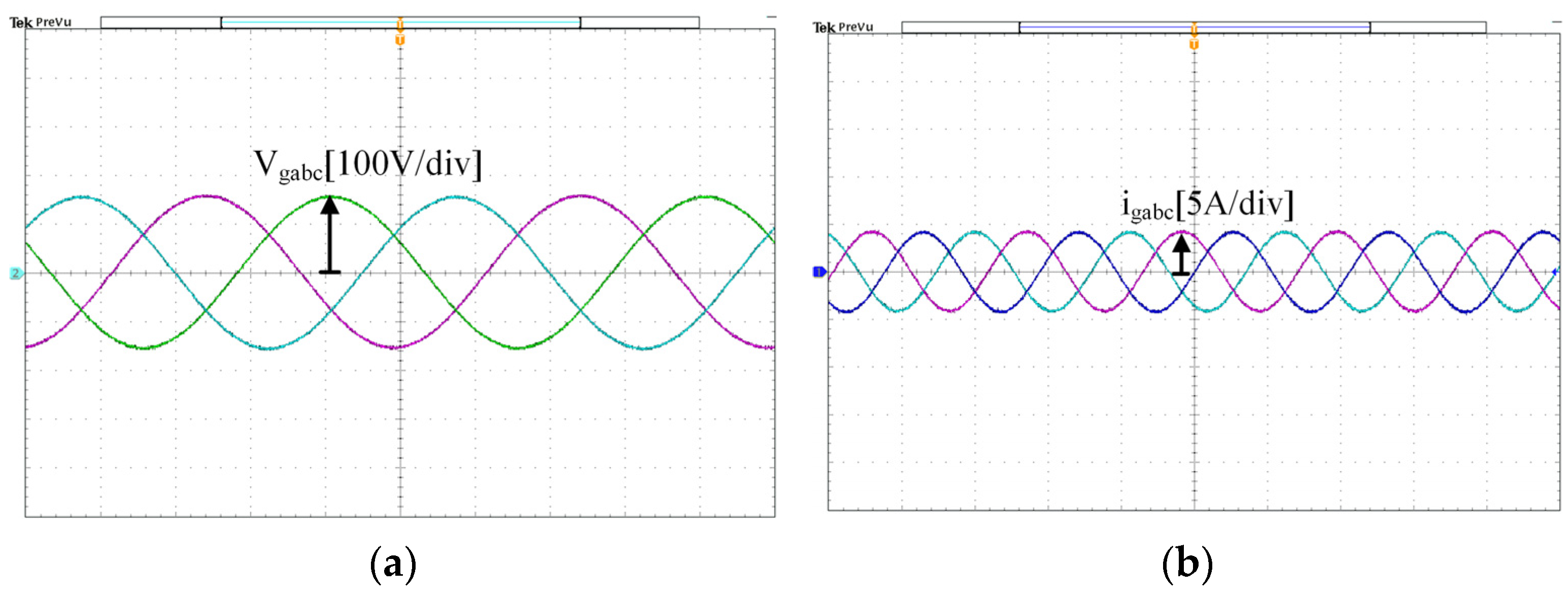
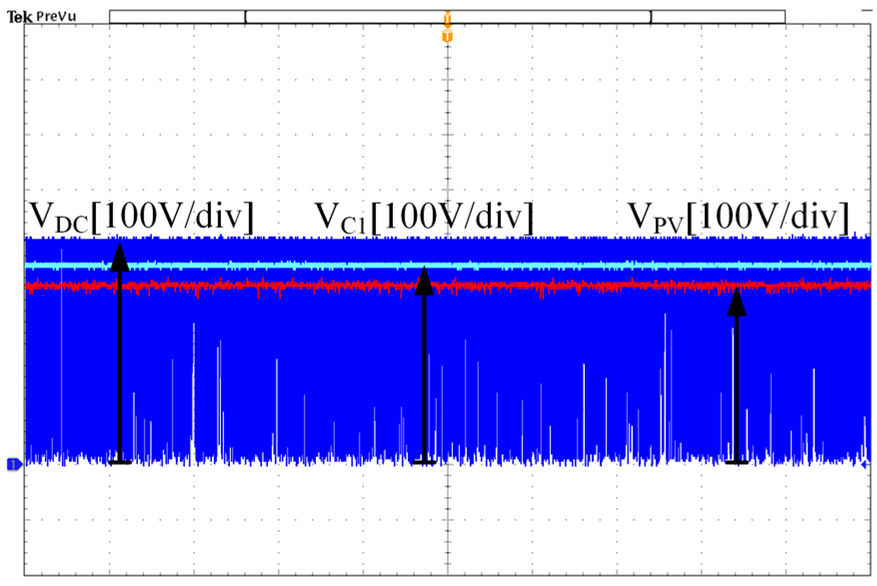
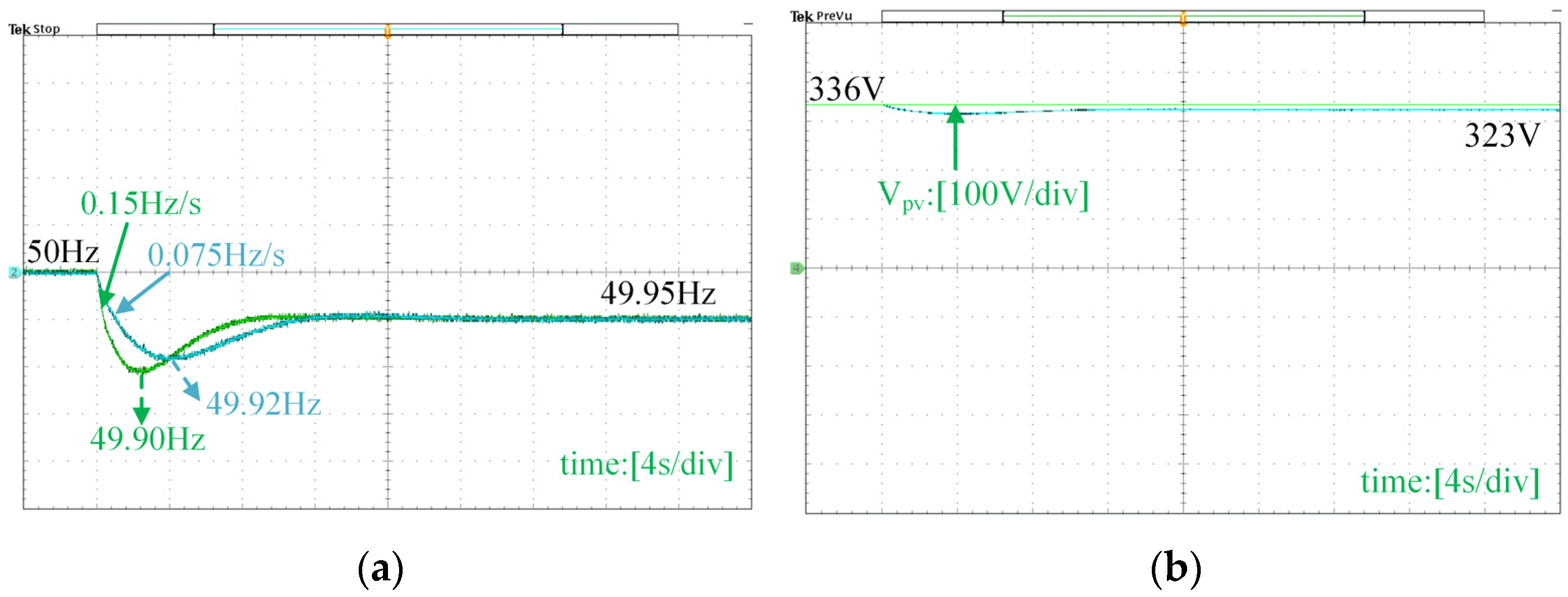
5.2. Experiment Verification

The experimental circuit built to verify the virtual inertia strategy is shown in Figure 18. In this circuit, the synchronous generator is replaced by a VSG, and the control algorithm of the VSG and quasi-Z-source grid-connected converter is implemented using the digital controller dSPACE hardware-in-the-loop simulation control platform. The VSG DC-link voltage vgdc is kept constant by using a constant voltage DC power supply, which then converts this voltage to AC voltage to simulate the grid voltage and provide a three-phase load bank with resistance RL.
The experiment was set up with a power of 1 kW, an AC output phase voltage of 110 V, a DC power supply output voltage of 335 V in normal operation, a switching tube operating frequency of 10 kHz, and a resistive load box. Sensors and AD acquisition were used to measure the grid-side voltage and current of the experimental prototype in real-time. Figure 19 shows the experimental waveform. vgabc in the figure represents the three-phase output voltage waveform of the VSG, with a peak voltage of 155.5 V and an effective voltage of 110 V. igabc is the three-phase output current, with a peak current of 4.28 A and an effective current of 3.03 A. The figure shows that the three-phase output voltage and current are smooth sinusoidal curves, which verifies that the VSG can provide stable three-phase AC power and simulate the power grid.
The quasi-Z-source power converter works in the inverted state when the voltage-frequency controller does not work, which is equivalent to the PV grid-connected experiment, and the experimental results are shown in Figure 20. The PV array in the experiment is simulated by using a DC power supply in series with a resistor, DC input voltage Vin = 336 V, and duty cycle D = 0.08. It can be seen from the figure that when the system is working stably, the voltage on capacitor C1 is VC1 = 368 V, while the voltage on capacitor C2 is VC2 = 32 V. The input inverter voltage is VDC = 400 V, which is the modulating waveform of the quasi-Z source, i.e., ZSVM2 modulated waveform. At this time, the PV array inputs 1 kW of active power to the grid.
The comparative experimental results of the two systems without and with virtual inertia under a 5% load addition are shown in Figure 21 when the proposed voltage-frequency controller is active. The quasi-Z-source power converter provides a virtual inertia of 5 s. Figure 21a shows that the system with virtual inertia has a lower RoCoF, changing from 0.15 Hz/s to 0.075 Hz/s under a 5% load change. This is a 50% improvement with virtual inertia. The maximum frequency deviation is also reduced from 0.12 Hz to 0.10 Hz, which is a 20% improvement. Figure 21b shows the voltage change on the capacitor Cpv during the load change. The DC-link voltage Vpv stays constant at 336 V without the proposed virtual inertia method. The voltage drops from 336 V to 323 V with the virtual inertia controller, and part of the energy released from the capacitor provides virtual inertia and buffers the frequency adjustment.
Similarly, the effect of virtual inertia under a different scenario of load reduction is shown in Figure 22. The comparative experimental results of the system without and with virtual inertia under a 5% load reduction are shown in the figure when the quasi-Z-source power converter provides 5 s of virtual inertia. Figure 22a shows that the system with virtual inertia has a lower RoCoF, changing from 0.15 Hz/s to 0.075 Hz/s. This is a 50% improvement with virtual inertia. The maximum frequency deviation is also reduced from 0.12 Hz to 0.10 Hz, which is a 20% improvement. However, the system frequency exceeds the nominal frequency of 50 Hz due to load reduction. Figure 22b shows the voltage change on the capacitor Cpv during the load reduction. Without the proposed method, the DC-link voltage Vpv stays constant at 336 V. With the virtual inertia controller, the voltage increases from 336 V to 349 V. The increased voltage on the quasi-Z-source capacitor is the energy absorbed from the grid, which reflects the same inertia boost and frequency support in the process.
The inertia analysis approach suggested in this study is substantiated by the experimental results, demonstrating its efficacy in accurately predicting key performance indicators of distributed power systems. These indicators include the rate of change of frequency (RoCoF), quasi-steady-state frequency, and DC-link voltage. It is important to acknowledge that the discrepancies observed between the projected values, simulation results, and experimental results may be attributed to model simplification and imprecise signal measurements. The virtual inertia model being presented is founded upon a quasi-Z-source power converter, which has the capability to be interconnected with either the low voltage grid or the medium voltage grid. The model has the capability to offer virtual inertia in both grid-connected and islanded operation modes, provided that the grid frequency can be measured at the point of common coupling (PCC). Hence, this method can be effectively employed in the context of the medium voltage grid, hence enhancing the frequency stability of power systems that possess a substantial integration of renewable energy sources.

6. Conclusions

This paper proposes and implements a novel virtual inertia scheme for distributed power systems using quasi-Z-source power converters. The scheme can enhance the frequency stability of the power system by utilizing the energy stored in the DC-link capacitors of the power converters. This paper also develops a virtual synchronous generator control strategy for the inverters to simulate the AC grid and provide grid support. The simulation and experimental results demonstrate that the proposed scheme can effectively improve the frequency response of the power system under different load scenarios, and the virtual synchronous generator can output a stable three-phase AC voltage. This paper contributes to the research and development of distributed power systems with high penetration of renewable energy sources, and provides a feasible and flexible solution for grid integration and grid support.

Author Contributions

Conceptualization, Y.L. and H.C.; methodology, R.F.; software, H.C.; validation, Y.L., H.C. and R.F.; formal analysis, H.C.; investigation, R.F.; resources, R.F.; data curation, Y.L.; writing—original draft preparation, Y.L.; writing—review and editing, Y.L.; visualization, H.C.; supervision, Y.L.; project administration, Y.L.; funding acquisition, Y.L. All authors have read and agreed to the published version of the manuscript.

Funding

This research was funded by [Shenzhen Science and Technology Program] grant number [JCYJ20200109105204077] and the APC was funded by [Shenzhen Science and Technology Program under Grant JCYJ20200109105204077].

Data Availability Statement

The data presented in this study are available per request from the corresponding author.

Conflicts of Interest

The authors declare no conflict of interest.

References

  1. Jurasz, J.; Canales, F.; Kies, A.; Guezgouz, M.; Beluco, A. A review on the complementarity of renewable energy sources: Concept, metrics, application and future research directions. Sol. Energy 2020, 195, 703–724. [Google Scholar] [CrossRef]
  2. Zongxiang, L.; Haiyan, T.; Ying, Q.; Xinshou, T.; Yongning, C. The impact of power electronics interfaces on power system frequency control: A review. Electr. Power 2018, 51, 51–58. [Google Scholar]
  3. Bera, A.; Chalamala, B.R.; Byrne, R.H.; Mitra, J. Sizing of energy storage for grid inertial support in presence of renewable energy. IEEE Trans. Power Syst. 2021, 37, 3769–3778. [Google Scholar] [CrossRef]
  4. Fang, J.; Li, H.; Tang, Y.; Blaabjerg, F. On the inertia of future more-electronics power systems. IEEE J. Emerg. Sel. Top. Power Electron. 2018, 7, 2130–2146. [Google Scholar] [CrossRef]
  5. Liu, F.; Liu, Z.; Mei, S.; Wei, W.; Yao, Y. ESO-based inertia emulation and rotor speed recovery control for DFIGs. IEEE Trans. Energy Convers. 2017, 32, 1209–1219. [Google Scholar] [CrossRef]
  6. Liu, R.; Wang, Z.; Xing, H. Virtual inertia control strategy for battery energy storage system in wind farm. In Proceedings of the 2019 IEEE PES Asia-Pacific Power and Energy Engineering Conference (APPEEC), Macao, China, 1–4 December 2019; pp. 1–5. [Google Scholar]
  7. Yan, W.; Wang, X.; Gao, W.; Gevorgian, V. Electro-mechanical modeling of wind turbine and energy storage systems with enhanced inertial response. J. Mod. Power Syst. Clean Energy 2020, 8, 820–830. [Google Scholar] [CrossRef]
  8. Martínez, J.C.; Gómez, S.A.; Amenedo, J.L.R.; Alonso-Martínez, J. Analysis of the frequency response of wind turbines with virtual inertia control. In Proceedings of the 2020 IEEE International Conference on Environment and Electrical Engineering and 2020 IEEE Industrial and Commercial Power Systems Europe (EEEIC/I&CPS Europe), Madrid, Spain, 6–9 June 2020; pp. 1–6. [Google Scholar]
  9. Zhang, X.; Yang, L.; Zhu, X. Virtual rotational inertia control of PV generation system with energy storage devices. Electr. Power Autom. Equip. 2017, 37, 109–115. [Google Scholar]
  10. You, F.; Si, X.; Dong, R.; Lin, D.; Xu, Y.; Xu, Y. A State-of-Charge-Based Flexible Synthetic Inertial Control Strategy of Battery Energy Storage Systems. Front. Energy Res. 2022, 10, 908361. [Google Scholar] [CrossRef]
  11. Fang, J.; Zhang, R.; Li, H.; Tang, Y. Frequency derivative-based inertia enhancement by grid-connected power converters with a frequency-locked-loop. IEEE Trans. Smart Grid 2018, 10, 4918–4927. [Google Scholar] [CrossRef]
  12. Karrari, S.; Baghaee, H.R.; Carne, G.D.; Noe, M.; Geisbuesch, J. Adaptive inertia emulation control for high-speed flywheel energy storage systems. IET Gener. Transm. Distrib. 2020, 14, 5047–5059. [Google Scholar] [CrossRef]
  13. Tian, B.; Gu, Y.; Wang, F.; Wang, X.; Yang, X. Virtual inertia dynamic control simulation model for renewable energy generation system. Renew. Energy 2018, 36, 1692–1696. [Google Scholar] [CrossRef]
  14. Fang, J.; Li, X.; Tang, Y.; Li, H. Design of virtual synchronous generators with enhanced frequency regulation and reduced voltage distortions. In Proceedings of the 2018 IEEE Applied Power Electronics Conference and Exposition (APEC), San Antonio, TX, USA, 4–8 March 2018; pp. 1412–1419. [Google Scholar]
  15. Shi, K.; Ye, H.; Song, W.; Zhou, G. Virtual inertia control strategy in microgrid based on virtual synchronous generator technology. IEEE Access 2018, 6, 27949–27957. [Google Scholar] [CrossRef]
  16. Wu, X.; Wei, Q. Virtual synchronous machine rotor angle droop control using virtual reactance. Electr. Technol. 2020, 21, 31–36. [Google Scholar]
  17. Chen, D.; Xu, Y.; Huang, A.Q. Integration of DC microgrids as virtual synchronous machines into the AC grid. IEEE Trans. Ind. Electron. 2017, 64, 7455–7466. [Google Scholar] [CrossRef]
  18. Shadoul, M.; Ahshan, R.; AlAbri, R.S.; Al-Badi, A.; Albadi, M.; Jamil, M. A comprehensive review on a virtual-synchronous generator: Topologies, control orders and techniques, energy storages, and applications. Energies 2022, 15, 8406. [Google Scholar] [CrossRef]
  19. Tamrakar, U.; Shrestha, D.; Maharjan, M.; Bhattarai, B.P.; Hansen, T.M.; Tonkoski, R. Virtual inertia: Current trends and future directions. Appl. Sci. 2017, 7, 654. [Google Scholar] [CrossRef]
  20. Zheng, X.; Liu, Y.; Pang, S.; Liu, Z.; Li, Y.; Wang, C. Sliding mode combined VSG control to microgrid inverters. In Proceedings of the IECON 2018-44th Annual Conference of the IEEE Industrial Electronics Society, Washington, DC, USA, 21–23 October 2018; pp. 2453–2456. [Google Scholar]
  21. Yan, X.; Wang, C.; Wang, Z.; Ma, H.; Liang, B.; Wei, X. A united control strategy of photovoltaic-battery energy storage system based on voltage-frequency controlled VSG. Electronics 2021, 10, 2047. [Google Scholar] [CrossRef]
  22. Babaei, E.; Abu-Rub, H.; Suryawanshi, H.M. Z-source converters: Topologies, modulation techniques, and application–part I. IEEE Trans. Ind. Electron. 2018, 65, 5092–5095. [Google Scholar] [CrossRef]
  23. Babae, E.; Suryawanshi, H.M.; Abu-Rub, H. Z-source converters: Topologies, modulation techniques, and applications—Part II. IEEE Trans. Ind. Electron. 2018, 65, 8274–8276. [Google Scholar] [CrossRef]
  24. Jeyasudha, S.; Geethalakshmi, B.; Saravanan, K.; Kumar, R.; Son, L.H.; Long, H.V. A novel Z-source boost derived hybrid converter for PV applications. Analog Integr. Circuits Signal Process. 2021, 109, 283–299. [Google Scholar] [CrossRef]
  25. Kundur, P.S.; Malik, O.P. Power System Stability and Control; McGraw-Hill Education: New York, NY, USA, 2022. [Google Scholar]
  26. Fang, J.; Li, H.; Tang, Y.; Blaabjerg, F. Distributed power system virtual inertia implemented by grid-connected power converters. IEEE Trans. Power Electron. 2017, 33, 8488–8499. [Google Scholar] [CrossRef]
  27. Konga, C.K.; Gitau, M. Three-phase quasi-Z-source rectifier modeling. In Proceedings of the 2012 Twenty-Seventh Annual IEEE Applied Power Electronics Conference and Exposition (APEC), Orlando, FL, USA, 5–9 February 2012; pp. 195–199. [Google Scholar]
  28. Liu, Y.; Ge, B.; Abu-Rub, H.; Peng, F.Z. Overview of space vector modulations for three-phase Z-source/quasi-Z-source inverters. IEEE Trans. Power Electron. 2013, 29, 2098–2108. [Google Scholar] [CrossRef]
Figure 1. Frequency response curve under a tripping of generator event.
Energies 16 06667 g001
Figure 2. Single-area power system structure.
Energies 16 06667 g002
Figure 3. Block diagram of power system frequency regulation.
Energies 16 06667 g003
Figure 4. Frequency response diagram under a 5% load addition. (a) Zero-pole diagram. (b) Frequency response graph.
Energies 16 06667 g004
Figure 5. Time-domain performance index of the system under a 5% load change (a) RoCoF, (b) frequency deviation, (c) overshoot, (d) adjustment time.
Energies 16 06667 g005
Figure 6. Three-phase QZSR topology.
Energies 16 06667 g006
Figure 7. Equivalent circuit of QZSR in two working states: (a) shoot-through state, (b) non-shoot-through state.
Energies 16 06667 g007
Figure 8. Inertia mapping from DC-link capacitors to a synchronous generator.
Energies 16 06667 g008
Figure 9. Quasi-Z-source grid-connected power converter with virtual inertia.
Energies 16 06667 g009
Figure 10. Three closed-loop control blocks of quasi-Z-source power converter.
Energies 16 06667 g010
Figure 11. The relationship between the maximum through duty cycle and the modulation ratio.
Energies 16 06667 g011
Figure 12. Block diagram of frequency adjustment with virtual inertia.
Energies 16 06667 g012
Figure 13. The relationship (a) between virtual inertia time constant, voltage, and maximum voltage deviation; (b) between virtual inertia time constant, voltage, and capacitance.
Energies 16 06667 g013
Figure 14. The three-phase output waveform of VSG: (a) output voltage, (b) output current.
Energies 16 06667 g014
Figure 15. Quasi-Z-source power converter output results: (a) quasi-Z-source capacitor voltage C1, C2, and Cpv; (b) input voltage of the QZSI; (c) shoot-through duty cycle D.
Energies 16 06667 g015
Figure 16. The frequency response curve of the system under a 5% load addition: (a) grid frequency, (b) DC-link capacitor voltage, (c) shoot-through duty cycle D.
Energies 16 06667 g016
Figure 17. The frequency response curve of the system under a 5% load reduction: (a) grid frequency, (b) DC-link capacitor voltage, (c) shoot-through duty cycle D.
Energies 16 06667 g017
Figure 18. Virtual inertia experiment platform diagram.
Energies 16 06667 g018
Figure 19. Three-phase output (a) voltage of VSG, (b) current of VSG.
Energies 16 06667 g019
Figure 20. Quasi-Z-source power converter output waveform.
Energies 16 06667 g020
Figure 21. Experimental results under a 5% load addition. (a) Frequency response, (b) voltage response.
Energies 16 06667 g021
Figure 22. Experimental results under a 5% load reduction. (a) Frequency response, (b) voltage response.
Energies 16 06667 g022
Table 1. Parameters’ value of power system.
DescriptionParameterValue
Droop coefficientR0.02
Rotor speed coefficientTG0.1 s
Turbine coefficientFHP0.3 s
Reheat engine time constantTRH7.0 s
Main inlet time constantTCH0.2 s
Inertia time constantH5 s
Rated frequencyfref50 Hz
Damping coefficientD1.0
Rated powerVArated1 kVA
Table 2. Parameters of quasi-Z-source power converter.
DescriptionParameterValue
Rated DC Chain VoltageVdc336 V
Max. DC Chain VoltageVpv_max390 V
Min. DC Chain VoltageVpv_min282 V
DC chain capacitanceCpv2.2 mF
Virtual inertia time constantHp5.0 s
Rated frequencyfref50 Hz
Max. frequency deviationΔfr_max0.2 Hz
Voltage-frequency controllerKfv270/40.2
Rated powerVArated1 kVA
Disclaimer/Publisher’s Note: The statements, opinions and data contained in all publications are solely those of the individual author(s) and contributor(s) and not of MDPI and/or the editor(s). MDPI and/or the editor(s) disclaim responsibility for any injury to people or property resulting from any ideas, methods, instructions or products referred to in the content.

