Narrow Band Frequency Response Analysis of Power Transformers with Deep Learning

Abstract

Frequency response analysis (FRA) is a standard technique for monitoring the integrity of the mechanical structure of power transformer windings. To date, however, there remains no suitable method for online testing using this technique. One of the main issues that persists is that any hardware designed to measure the frequencies in the range of interest would filter out frequency bands used for assessment by humans. The growth of pattern recognition capabilities in deep learning networks, however, now offers the possibility of detecting different types of faults in a narrow frequency band, which is simply not possible for human experts. This paper explores the ability of a selection of typical networks to classify common faults within different bands. The results show that networks are able to identify faults in bands where humans are unable to find them, which has implications for signal processing and electronics design in developing a system for online monitoring.

1. Introduction

Frequency Response Analysis (FRA) is considered to be one of the most reliable methods for assessing the mechanical integrity of power transformer windings [1]. The most common approach, Sweep Frequency Response Analysis (SFRA), involves applying a low-voltage reference signal V_in to one transformer terminal and measuring the response signal V_out at another terminal for a range of frequencies [2]. The result of this is the transformer’s frequency response (FR), which contains multiple resonances representing the relative magnitudes and couplings between the internal RLC components. Changes or faults in a transformer winding change the balance of R, L, and C components, causing the frequency response to change [3]. Typically, magnitude and phase measurements are taken during SFRA, and interpretation relies on experts who visually inspect FRs to determine the type and severity of any winding fault. However, this method is time-consuming, inconsistent, and dependent on experts who assess damage to the core, windings, and leads of the transformer by visually examining the frequency response, which ranges between 2 Hz and 2 MHz.

Usually, experts consider core issues to manifest in low frequency, windings in the mid-band range, and leads and bushing issues in the upper range. Tests are exclusively carried out with the transformer offline, and there has been little progress in advancing the field to online monitoring beyond the lab.

One of the major issues to contend with is the wide frequency range required. While studies [4,5] have found methods to inject high-frequency signals into transformers online, a usable measurement technique remains elusive. This is because the low frequency band typically extends power frequency below the 60 Hz, making it impossible or prohibitively expensive to extract readings in this range.

Deep learning (DL) is a subset of machine learning that involves the use of artificial neural networks with multiple layers to analyze and learn from complex data [6]. In recent years, there has been growing interest in the use of deep learning techniques in the field of transformer frequency response analysis (FRA), as these techniques can help to improve the accuracy and efficiency of analysis. One of the main applications of deep learning in transformer FRA is fault detection and diagnosis. This is where neural networks are trained on large datasets of transformer frequency response data to identify patterns and anomalies that may indicate the presence of faults or defects in the transformer. By analyzing the frequency response data in this way, deep learning models can help to identify faults much more quickly and accurately than traditional methods.

One common technique in Series Data Classification (SDC) is to convert series data into images, as seen in previous studies such as [7]. This approach is motivated by the impressive performance of 2D Convolutional Neural Networks (CNN) for image classification [8]. In this study, both image and series data representations were used to analyze different frequency ranges, allowing for a comparison of NN performance between the two formats. The aim was to identify differences in performance and ultimately determine which format is better to use for a given task.

Previous studies on transformer frequency response ranges have primarily focused on determining the impact of transformer model parameter variations on frequency response. For example, studies such as [9,10] have reported sensitivity studies to determine the effect of various model parameters on FRA signatures.

In this study, we first aimed to determine whether deep learning networks are able to identify faults using narrow frequency bands in the mid- and high-frequency regions of the SFRA response, and second to determine whether there is a particular range in which the distinguishing features of the plots are strongest. These studies are necessary precursors to the design and optimization of hardware capable of measuring online SFRA response bands with sufficient information to function effectively as monitoring devices. Additionally, different data representations such as image and series data and the magnitude, and phase of sweep frequency response analysis (SFRA) measurements were examined in order to gain insights into how deep learning techniques can be optimized for different frequency response ranges of transformers as a means of improving the accuracy of FRA and fault diagnosis.

The remainder of this paper is organized as follows: Section 2 outlines the overview of the system design and explains the proposed methodology; Section 3 presents performance metrics and the results of the designed models; finally, Section 4 summarises the main findings and suggests avenues for future work.

2. Methods

2.1. SFRA Data Generation

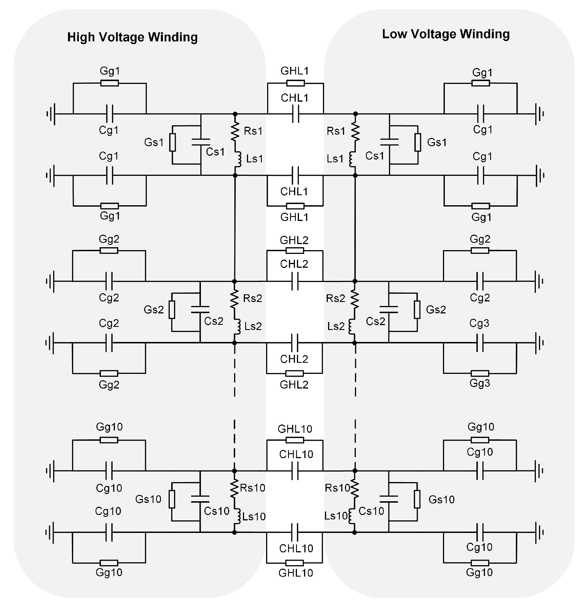
Deep neural networks rely on large datasets to perform well [6]. However, creating models of faults on an actual transformer can be costly and destructive. Hence, simulation studies must be conducted for exploration purposes. Transformer modelling involves creating mathematical models that simulate the behaviour of a physical transformer. The transformer model typically includes representations of the transformer winding as well as other components such as the insulation and tank. While various models have been developed to preserve geometric representation, in this we study utilize the well-established lumped ladder model with ten segments (as shown in Figure 1), as it has been demonstrated to produce good agreement with measured responses [11].

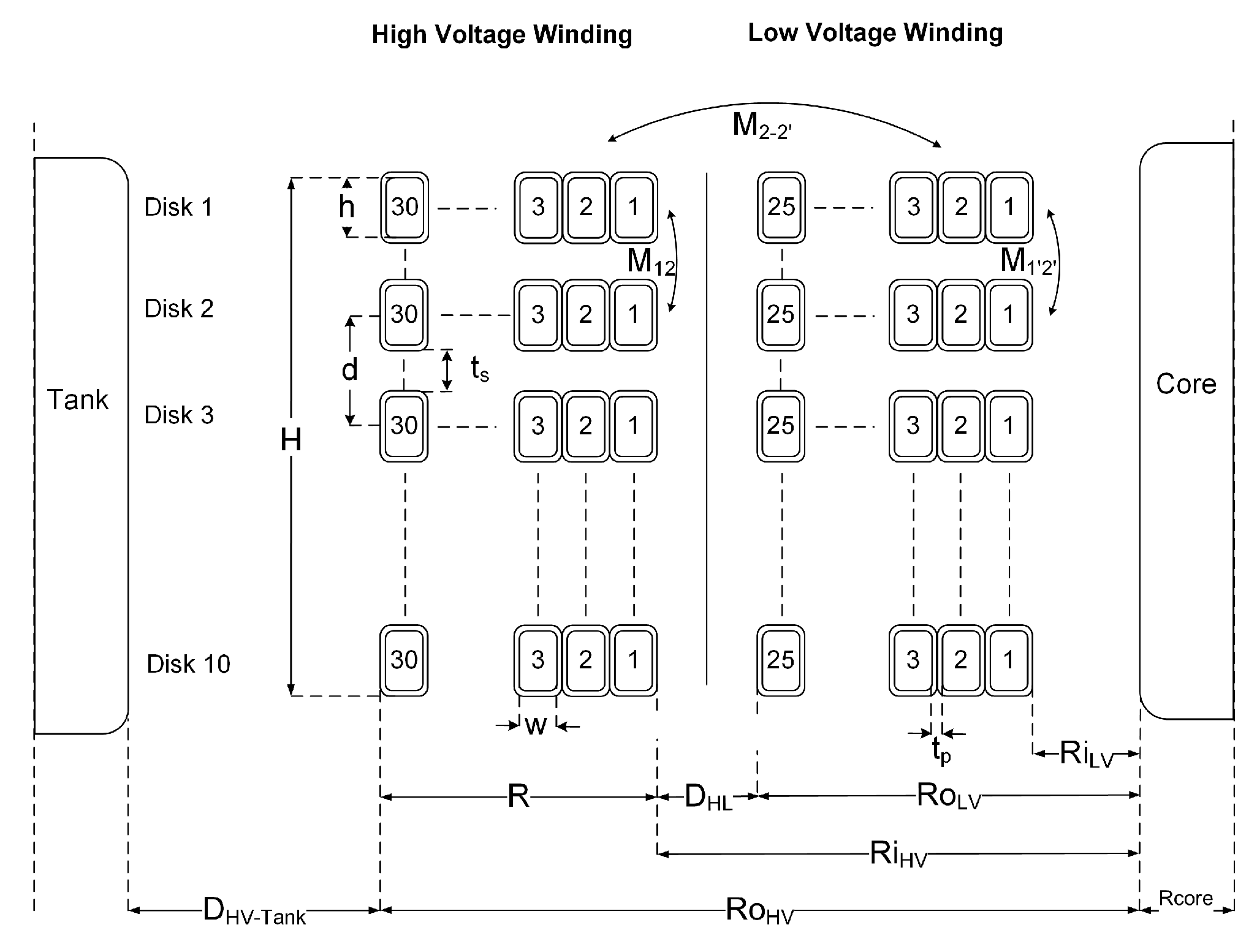
To calculate the parameters of the ladder model, the dimensions of a 33/11 kV 30 MVA power transformer were used, as presented in [9]. The spatial measurements can be found in

Table 1. Transformer winding measurements.

Measurement	Symbol	HV (mm)	LV (mm)
Conductor width	w	2.4	7.2
Conductor height	h	11.5	27.3
Insulation thickness	$t_p$	0.5	0.5
Distance between layers	$t_s$	5.0	5.0
Outer winding radius	$R_o$	466.5	355.5
Inner winding radius	$R_i$	374.5	275.5
Dist. between HV and LV winding	$D_{HV-LV}$	20.0
Dist. between LV and core	$D_{LV-Core}$	15.0
Dist. between HV and Tank	$D_{HV-Tank}$	92.0

, while a detailed cross-sectional view of the transformer winding is shown in Figure 2.

2.1.1. Calculating the Series Capacitance

According to the theory presented in [12], the total series capacitance of a continuous winding is determined by adding the inter-turn capacitance $C_{tt}$ and the inter-disk capacitance $C_{dd}$ as provided by Equations (1) and (2), respectively.

$$C_{tt}=\frac{{ϵ}_p{ϵ}_0{D}_m\pi (h+t_p)}{t_p}$$

(1)

$$C_{dd}={ϵ}_0\left(\frac{k}{\frac{t_p}{{ϵ}_p}+\frac{t_s}{{ϵ}_{oil}}}+\frac{1-k}{\frac{t_p}{{ϵ}_p}+\frac{t_s}{{ϵ}_s}}\right)\pi D_m(R+t_s)$$

(2)

where $D_m$ represents the mean diameter of the winding, h is the height of the conductor, R is the radial depth of the winding, $t_p$ denotes the thickness of the paper insulation on both sides, ${ϵ}_p$ represents the relative permittivity of the insulating paper, ${ϵ}_0$ is the permittivity of free space, ${ϵ}_s$ is the permittivity of the disk spacer, ${ϵ}_{oil}$ is the permittivity of the transformer oil, and k indicates the proportion of circumferential space occupied by oil.

The calculation of the inter-turn capacitance and inter-disk capacitance follows the sum of energy principle as described in [12]. According to this principle, the total energy of the disk coil is equal to the sum of the individual capacitances within the disk. For a pair of disks with N conductor turns, there will be $2N-2$ inter-turn capacitors. The total resultant inter-turn capacitance between conductors is provided by Equation (3), and the resultant inter-disk capacitance is provided by Equation (4).

$$C_T=\frac{1}{2}{C}_{tt}\left(\frac{N-1}{N^2}\right)$$

(3)

$$C_D=\frac{C_{dd}}{3}l$$

(4)

The series capacitance between a disk pair $C_s$ is a sum of the resultant inter-turn capacitance $C_T$, and the resultant inter-disc capacitance $C_D$ as shown in Equation (5).

$$C_s=C_T+C_D$$

(5)

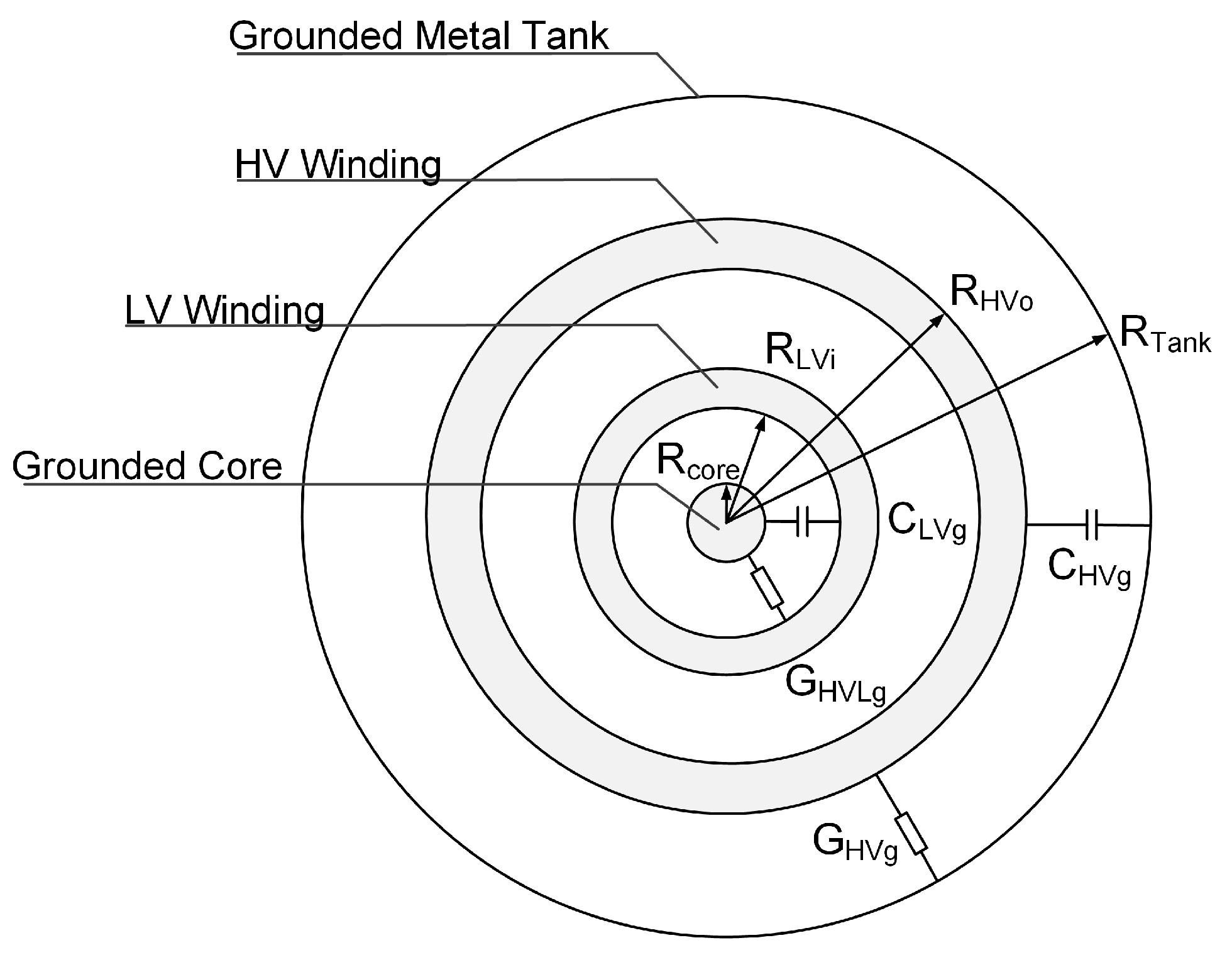
2.1.2. Calculating Ground Capacitance

To calculate the ground capacitance, the formula for capacitance between concentric cylinders was used. Referring to Figure 3, the ground capacitance between the HV winding can be calculated using (6), while the ground capacitance between the LV winding and the core can be calculated using (7), considering that the tank and the core are both grounded.

$$C_{HVg}=\frac{2\pi {ϵ}_r{ϵ}_{0}H}{ln\frac{R_{HVo}}{R_{Tank}}}$$

(6)

$$C_{LVg}=\frac{2\pi {ϵ}_r{ϵ}_{0}H}{ln\frac{R_{LVi}}{R_{Core}}}$$

(7)

2.1.3. Calculating Conductance

To calculate the ground conductance for the HV and LV windings, the ground capacitance was first determined and then used in Equations (8) and (9). The values for $tan\delta$ (the insulation dissipation factor) and f (the frequency) were taken into consideration.

$$G_{HVg}=2\pi f{C}_{HVg}tan\delta$$

(8)

$$G_{LVg}=2\pi f{C}_{LVg}tan\delta$$

(9)

Similarly, the HV and LV series conductance were calculated using Equations (10) and (11).

$$G_{HVs}=2\pi f{C}_{HVs}tan\delta$$

(10)

$$G_{LVs}=2\pi f{C}_{LVs}tan\delta$$

(11)

2.1.4. Calculating Series Resistance

The series resistance was calculated using Equations (12) and (13), which take the frequency and conductor permeability into consideration [9]:

$$R_{s1}^{\prime }=\frac{1}{2(h+w)\sqrt{\frac{\pi f\mu }{\sigma }}}$$

(12)

$$R_{s1}=R_{s1}^{\prime }\times l_{Cir}$$

(13)

where $l_{Cir}$ is the total circumference of the winding conductor, h is the conductor height, $\mu$ is the conductor permeability, and $\sigma$ is the conductivity.

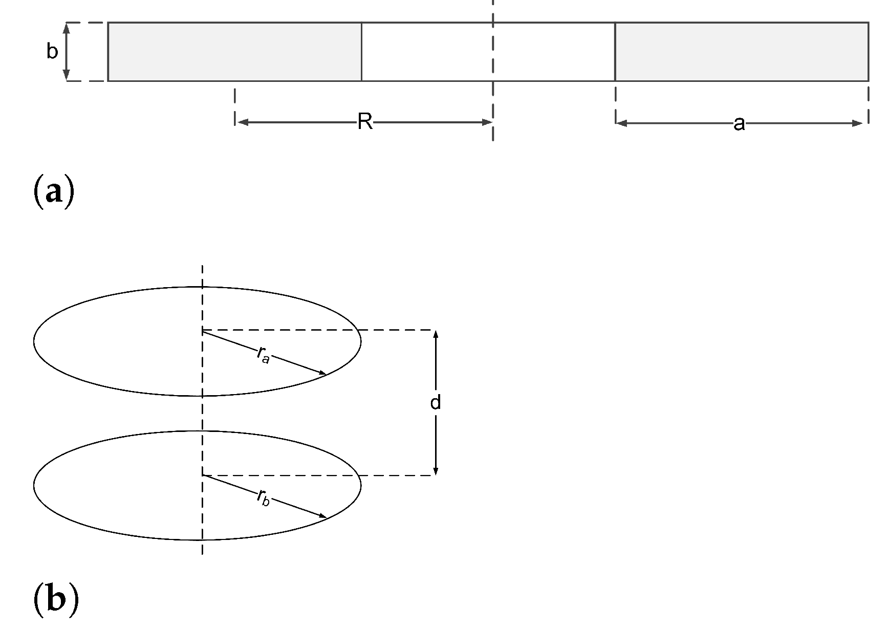
2.1.5. Calculating Self and Mutual Inductance

Figure 4a depicts a cross-sectional view of a single conductor loop. The self-inductance can be calculated using the formula provided in [13], as shown in (14), where a is the radial depth of the conductor, b is the axial length of the conductor, and R is the average radius of the winding. Additionally, the Geometric Mean Distance (GMD) can be determined using Equation (15).

$$L_s={\mu }_{0}R(ln\frac{8R}{GMD}-2)$$

(14)

$$GMD=\sqrt{a^2-b^2}{e}^{\left[\frac{2b}{3a}{tan}^{-1}\left(\frac{a}{b}\right)+\frac{2a}{3b}{tan}^{-1}\left(\frac{b}{a}\right)-\frac{b^2}{12a^2}ln(1+\frac{a^2}{b^2})\right]}$$

(15)

Figure 4b depicts two conductor loops with radii $r_a$ and $r_b$ separated by a distance of d. The mutual inductance between the winding disks was calculated using (17). This equation involves the complete elliptic integrals of the first and second kind, denoted as $K\left(k\right)$ and $E\left(k\right)$, respectively. The formula used to calculate the mutual inductance is derived from the expression for mutual inductance between two thin wire coaxial loops, as explained in [12].

$$M_{ab}=\frac{2{\mu }_0\sqrt{r_a{r}_b}}{\sqrt{k}}\left(E\left(k\right)-\left(K\right(k)\right)$$

(16)

$$k=\sqrt{\frac{4r_a{r}_b}{{(r_a+r_b)}^2+d^2}}$$

(17)

The ladder model was simulated using a custom written Frequency Domain Nodal Analysis Solution coded in MATLAB. This was preferred to using existing circuit simulation software to make it easier to automate the workflow of changing the model parameters, simulating, labelling, and then storing data for further processing.

2.2. Fault Modeling

Winding faults occur due to changes in a winding’s physical, structural, or material properties. Therefore, to simulate these faults, it is possible to change the base properties of the winding on the ladder model to mimic faulted conditions [14,15]. This change in the winding properties would result in a change in the winding parameters, and consequently the frequency response (FR). The simulation process was carried out for six different fault cases, including dielectric leakage current faults (DLFs), inter-disk displacement faults (IDFs), radial displacement faults (RDFs), short-circuit faults (SCFs), loss of clamping pressure faults (LCFs), and non-faults (NFs). This section describes the simulation process for each of the fault cases.

Radial displacement faults (RDFs) refer to cases in which parts of a winding are shifted in the radial direction. To simulate this type of fault, the mean radius of the disks in the HV winding, denoted as $R_m$, was varied by ±10%. The original value of $R_m$ was 420 mm; thus, the maximum expansion or contraction was ±42 mm. This range was considered practical in light of the transformer’s surrounding geometry.

An IDF happens when there is an increase in the space between winding sections. In this study, these fault were simulated by adjusting the inter-disk distance $d_{pb}$ by 0–100%. Although previous studies [16,17] have simulated IDFs with disk spaces increasing beyond 300%, the range used in this study was limited to 0–100% (3 mm–6 mm) to account for less severe IDFs.

LCFs are caused by mechanical hysteresis in the pressboard, which increases the conductivity between the winding disks. To simulate this fault, the insulation dissipation factor $tan\delta$ was increased, thereby increasing the series conductance $G_s$.

Similarly, DLFs occur due to an increase in leakage current to the earth. This fault was simulated by increasing the ground conductance $G_g$ by increasing the $tan\delta$. In this study, $tan\delta$ was increased up to 80% for both LCFs and DLFs, as previous studies [18] have shown that $tan\delta$ can reach up to 80% when the winding paper insulation becomes moist.

To simulate SCFs, short-circuit connections were inserted between the affected disks. These faults can occur with different short circuit impedance. To simulate this, the value of $R_{sc}$ was varied between 10–1000 $\Omega$.

To train the NNs, data for non-fault (NF) cases were required. The frequency response (FR) for these cases needed to be sufficiently different to avoid generating duplicate sweep frequency response analysis (SFRA) data while remaining within an acceptable range of the base FR. The statistical index known as the correlation coefficient (CC), which is recommended in the IEEE standard C57.149 [2], was used to achieve this. The calculated parameters were varied until the CC values for the low, middle, and high frequency bands of all the NF fault cases were above the specified threshold value of 0.9998.

To simulate the fault location, each possible disk on the winding was iterated through while changing the number of affected surrounding disks. The frequency response for each case had a resolution of 5000 points between the frequency range of 1 KHz–2 MHZ, which is in accordance with IEEE standard C57.149 [2]. The entire fault simulation process generated 24,000 fault cases. For a summary of this process, refer to

Table 2. Summary of fault simulation.

Fault Case	Changed Property	Symbol	Variation	No. Cases
RDF	Mean radius	$R_s$	±10%	4400
IDF	Inter-disk distance	d	100%	9000
LCF	Insulation dissipation factor	$tan\delta$	0–80%	4400
DLF	Insulation dissipation factor	$tan\delta$	0–80%	4400
SCF	Short circuit impedance	$R_{sc}$	10–1000 $\mathrm{\Omega }$	5500
NF	-	-	$0.0005$%	4400

.

2.3. Data Preprocessing

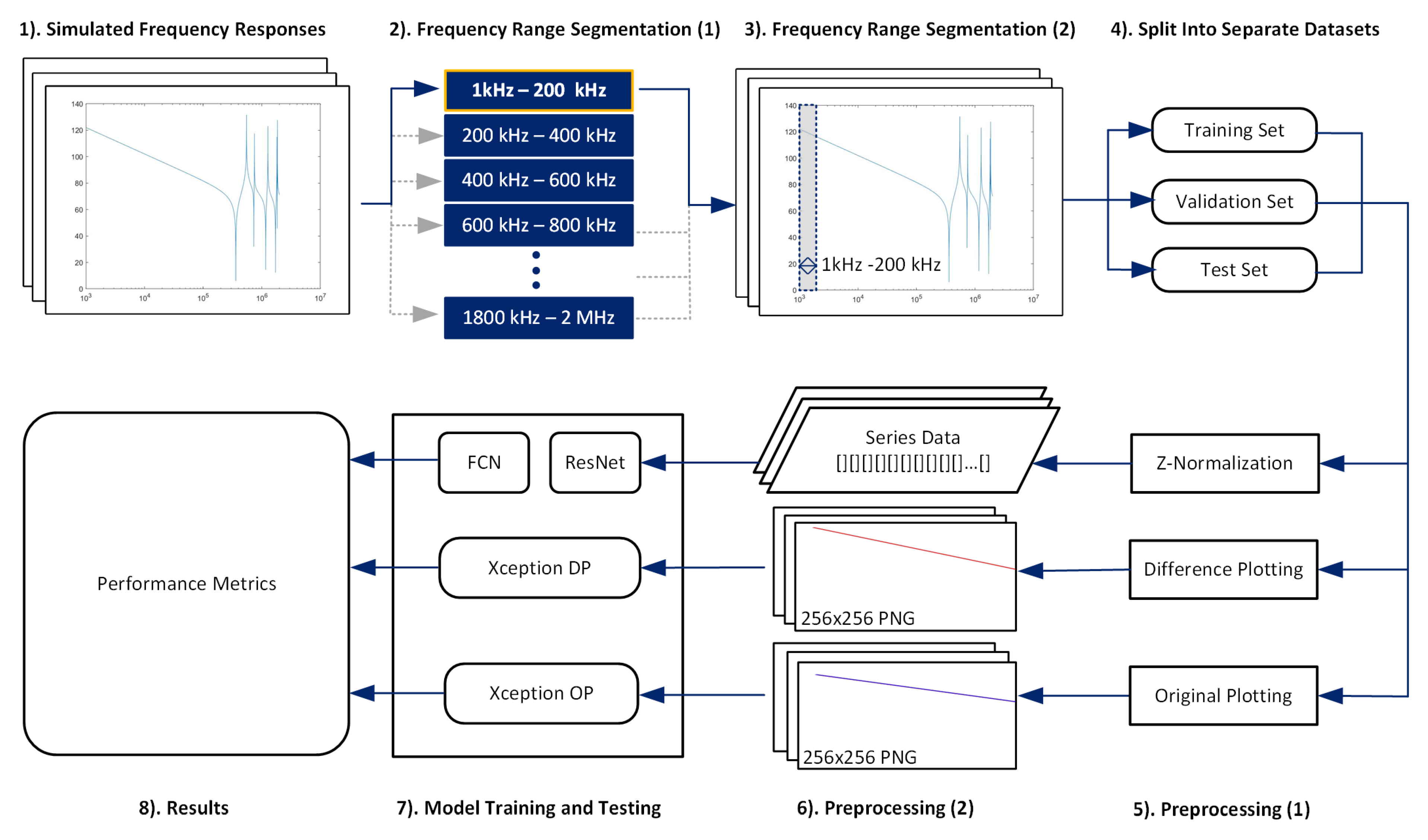
To investigate the performance of the neural networks over different frequency ranges, each frequency response (FR) was divided into 200 kHz intervals, as illustrated in Figure 5. After segmentation, the FRs were split randomly, with 80% used for training, 10% for validation, and 10% for testing. Because the datasets were sufficiently large, this random split resulted in an even class distribution. This study explored both series and image data representations of the FRA data. For the series data, only z-normalization was applied, which is a typical preprocessing step. Two types of image representations were used: Original Plot (OP) and Difference Plot (DP) images. The OPs were a reconstruction of the FRA bode plot with only a single plot on the axes. This type of analysis would be virtually impossible for humans, as there is no baseline plot for comparison on the graph. Neural networks, however, are able to use the axis limits themselves as a frame of reference, and do not need to “see” the reference plot on the same axes. The DPs were produced by plotting both the reference trace and the faulted trace, then shading the difference between them to be closer to what a human expert is able to analyze. The image data had a resolution of 256 × 256 in Portable Network Graphics (PNG) format, as lossless compression was used. The preprocessing and NN training were implemented in Python 3.8 and TensorFlow 2.5.

2.4. NN Training

In this study, we investigated three neural network architectures: Xception was trained with image FRA data, while ResNet and FCN were both trained using series FRA data. At its core, fault classification using SFRA data is a Series Data Classification (SDC) task. There have been many NNs proposed over the years for SDC. In [19], nine NNs were compared for SDC, and it was concluded that the Residual Neural Network (ResNet) performed the best, followed by the Fully Convolutional Neural Network (FCN). However, these findings contradicted earlier research in [20] which suggested that FCN outperformed ResNet. For this reason, this study tested ResNet and FCN using series FRA data. This section briefly describes the architecture of each NN.

2.4.1. FCN

FCN stands for Fully Convolutional Network, which is a type of neural network designed specifically for semantic segmentation tasks. The architecture of FCN is based on a modified VGG-16 architecture. However, instead of using fully connected layers at the end of the network to produce a single output, FCN replaces those layers with convolutional layers. This architecture contains three convolution blocks, each followed by batch normalization to enhance generalization and speed up convergence. We used a global average pooling layer before the final SoftMax layer to reduce the number of weights [20].

2.4.2. ResNet

ResNet is a deep neural network architecture that was introduced by Microsoft Research Asia in 2015. It is designed to address the vanishing gradient problem that occurs in very deep neural networks. ResNet uses skip connections to allow information to flow directly from the input to the output, bypassing intermediate layers. This helps to mitigate the problem of gradients becoming very small and allows for the training of very deep networks. The version we used contained three residual blocks followed by a global average pooling layer and a SoftMax classifier [20]. Each residual block contains three convolutions, after which the output is added to the residual bock’s input and fed to the next layer, followed by a ReLU activation function and a batch normalization operation [19].

2.4.3. Xception

Xception is a deep convolutional neural network proposed in [21] as an extension of the Inception architecture. It comprises 36 hidden layers and up to 22.6 M parameters. The Xception architecture employs depthwise separable convolution layers that separate the spatial and channel-wise filtering, reducing the number of parameters needed to train the model and improving efficiency [22]. This architecture includes skip and residual connections to mitigate the vanishing gradient problem and improve performance. Xception is modular and flexible, making it adaptable to different tasks and datasets, and has achieved state-of-the-art results in computer vision tasks such as image classification, object detection, and semantic segmentation. In this study, we used a version of Xception pretrained on the ImageNet dataset [23].

The hyperparameters of each NN were tuned using the Hyperband tuning algorithm from the Keras Tuner library [24]. The Hyperband tuning algorithm uses a principled early-stopping strategy that allocates more resources to promising hyperparameter configurations while eliminating poor ones. This makes Hyperband more efficient than alternative approaches such as Random Search and Bayesian optimization. The search space for the tuner included the learning rate, dropout rate, and batch size, as well as the hidden layers for Xception. The Hyperband operation ran on each model for a total of 75 trials, allowing a sufficient number of hyperparameter combinations to be tested.

Table 3. Tuned NN Hyperparameters.

Architecture	FRA Measurement	Learning Rate	Dropout Rate	Batch Size	No. of Hidden Layers	Layer1 Node No.	Layer2 Node No.	Layer3 Node No.
Xception-DP	Mag.	0.005	0.7	32	2	288	480	NA
	Phase	0.003	0.5	48	2	480	352	NA
Xception-OP	Mag.	0.05	0.45	48	3	160	96	416
	Phase	0.003	0.65	48	3	449	160	384
FCN	Mag.	0.001	0.75	32	NA	NA	NA	NA
	Phase	0.001	0.8	32	NA	NA	NA	NA
ResNet	Mag.	0.007	0.8	32	NA	NA	NA	NA
	Phase	0.009	0.55	32	NA	NA	NA	NA

shows the tuned hyperparameter values for each model. All models evaluated in this study used the adaptive learning rate through the adaptive moment estimation (Adam) optimizer.

2.5. Performance Metrics

To assess the performance of the networks, Precision and Recall were calculated as follows (Figure 6):

$$P=\frac{TP}{TP+FP}$$

(18)

$$R=\frac{TP}{TP+FN}$$

(19)

where P and R are the Precision and Recall, respectively, $TP$ is the number of True Positives, $FP$ is the number of False Positives, and $FN$ is the number of False Negatives. These categories were all known a priori for the entire data set, as it was generated via simulation.

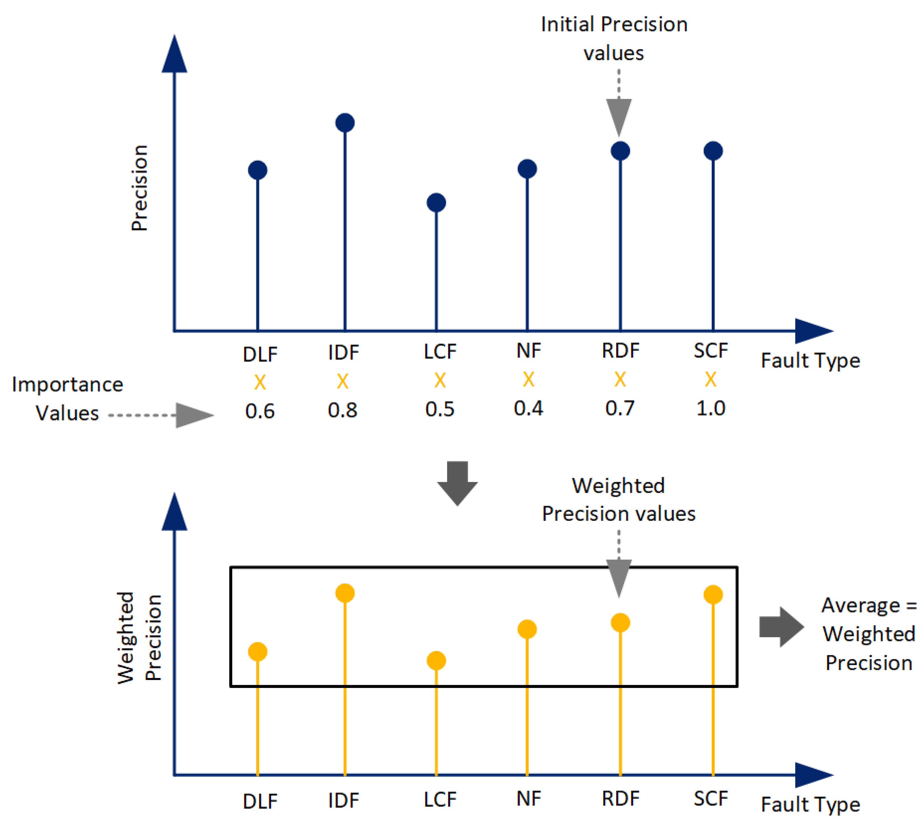
A low Precision indicates that the network is detecting instances of faults where there are none (false alarms), while a low Recall indicates that the network is not detecting faults as it should (missed detections).

Typically, both metrics are combined. However, because missed detections have more severe consequences than false alarms when dealing with faults, it is preferable to keep the metrics separate, using Recall as the primary measure and examining the Precision afterwards. Additionally, when assessing the performance of a neural network all classes are usually given equal importance. However, in this case, certain winding faults are more critical than others. For instance, an SCF is considered the most severe winding fault, and can have catastrophic consequences if not addressed; on the other hand, a DLF is not considered as severe an occurrence. To compensate for this disparity between the severity of different faults, the average weighted Precision and Recall scores (Equations (20) and (21)) were calculated as follows:

$$P_{w,avg}=\frac{1}{N}\sum _{F=0}^N{P}_F{I}_F$$

(20)

$$R_{w,avg}=\frac{1}{N}\sum _{F=0}^N{R}_F{I}_F$$

(21)

where $P_{w,avg}$ and $R_{w,avg}$ are the average weighted Precision and Recall values, N is the number of faults, F is the fault number from

Table 4. Assigned importance values.

Fault Number	Fault Type	Abbreviation	Importance
1	Short Circuit Fault	SCF	1
2	Inter-Disk displacement Fault	IDF	0.8
3	Radial displacement Fault	RDF	0.7
4	Dielectric leakage current Fault	DLF	0.6
5	Loss of Clamping Pressure	LCF	0.5
6	No-Fault	NF	0.4

, $P_F$ is the precision of fault F, and $I_F$ is the importance of fault F from Table 4.

The importance value ascribed to each fault is subjective, and was determined through consultation with testing personnel in the field. The values of $P_{w,avg}$ and $R_{w,avg}$ were calculated for each network in each frequency band.

3. Results

When a new FR band is input to any of the networks, the network classifies it into one of the fault (or no fault) categories.

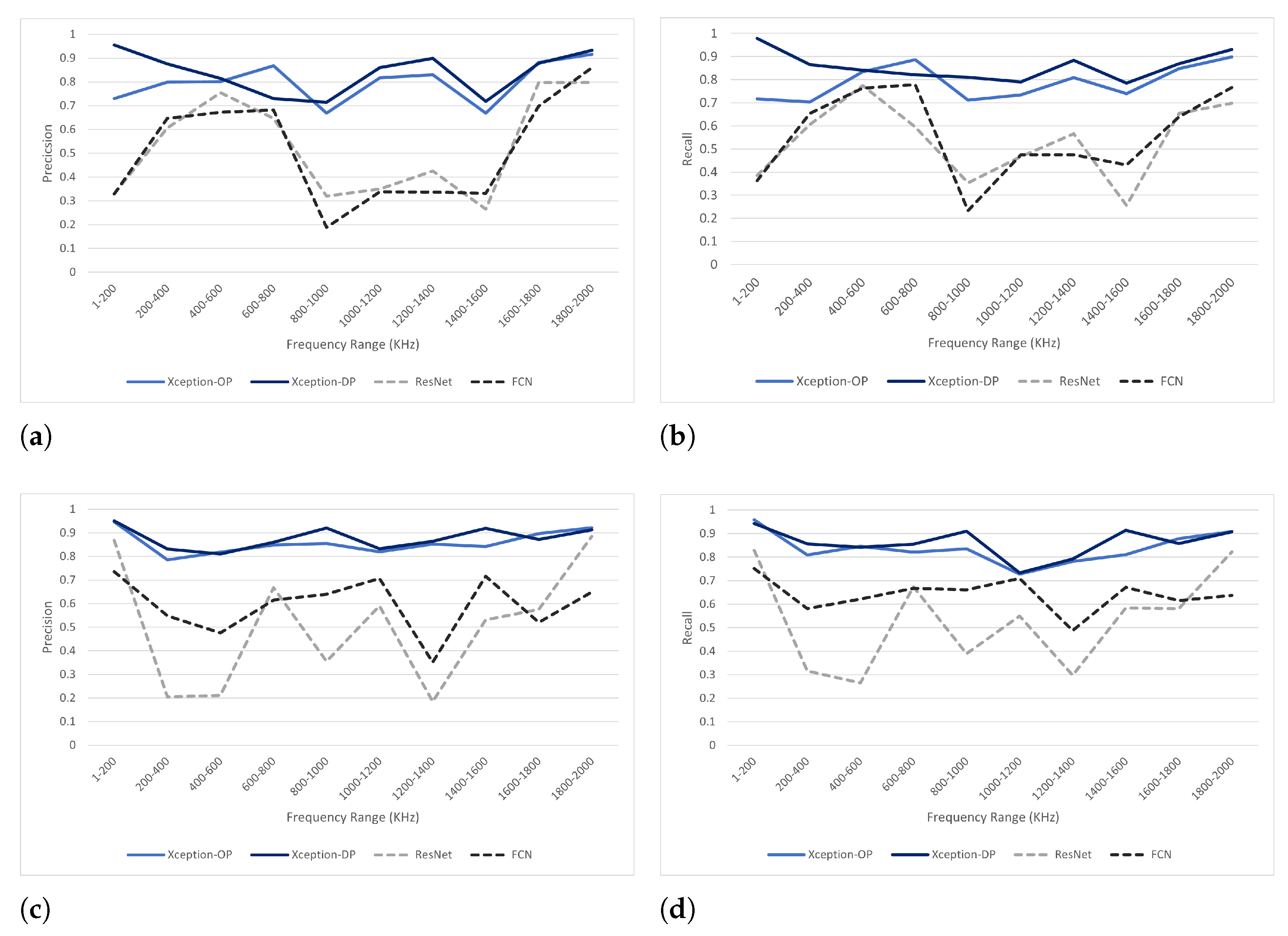
The performance of the neural networks across different frequency response ranges is illustrated in Figure 7. Surprisingly, the networks achieved relatively high performance even when trained on significantly reduced frequency response range data. The precision and recall values for some frequency response ranges were almost as high as those obtained when using the entire frequency response (100 KHz–2 MHz).

These findings indicate that although faults are typically looked at in particular frequency ranges by humans, their effects result in distinguishable features throughout the frequency spectrum of the impedance plots. This is a significant finding, as a robust online monitoring technique would be required to filter out power, harmonic, and noise frequencies. If the fault features were not distinguishable throughout the spectrum, this would render online techniques blind to faults which manifest predominantly in those ranges. The ability of deep learning classifiers to distinguish features in ranges where they may not be most prominent allows the use of band-limited measurement devices without sacrificing the ability to detect any faults, as opposed requiring to the wide ranges recommended by various expert bodies such as the IEC [25] and CIGRE [26].

Our results indicate that the neural networks (NNs) trained using images (Xception OP and Xception DP) performed better than those trained using series data (FCN and Resnet) for all frequency response ranges, achieving higher precision and recall values. This aligns with the findings of a previous study [7], which suggested that 2D CNN architectures trained using image-encoded series data outperformed 1D CNN architectures trained using traditional series data. Nonetheless, there may be other factors that influenced this difference in performance.

One possible reason why the neural networks trained with images (Xception OP and Xception DP) outperformed those trained with series data (FCN and Resnet) is because of the architecture depth. Xception has a significantly deeper architecture compared to FCN and ResNet, which can be an advantage when dealing with complex learning problems, as shown in [22]. This is because deeper neural networks have more layers, making them capable of learning more complex features and representations of the input data. In contrast, shallow networks with fewer layers may not have enough capacity to learn these complex features, and can be limited in their ability to accurately model the input-output mapping.

Furthermore, among the three models analyzed in the study only Xception employed pretrained weights. These Pretrained weights may have allowed Xception to learn pertinent features from the vast number of images in the ImageNet database, improving the model’s generalization and performance. This finding is consistent with the research conducted in [27], which emphasized the advantages of transfer learning in deep neural networks.

Another notable observation is that the neural networks achieved the highest precision and recall scores in the 100 kHz–200 kHz and 1.8 MHz–2 MHz ranges, which correspond to the lowest and highest regions of the frequency response, respectively. This is interesting because it suggests that although artefacts may show up visually in different frequency bands, there are features across the entire range of frequencies that can be extracted.

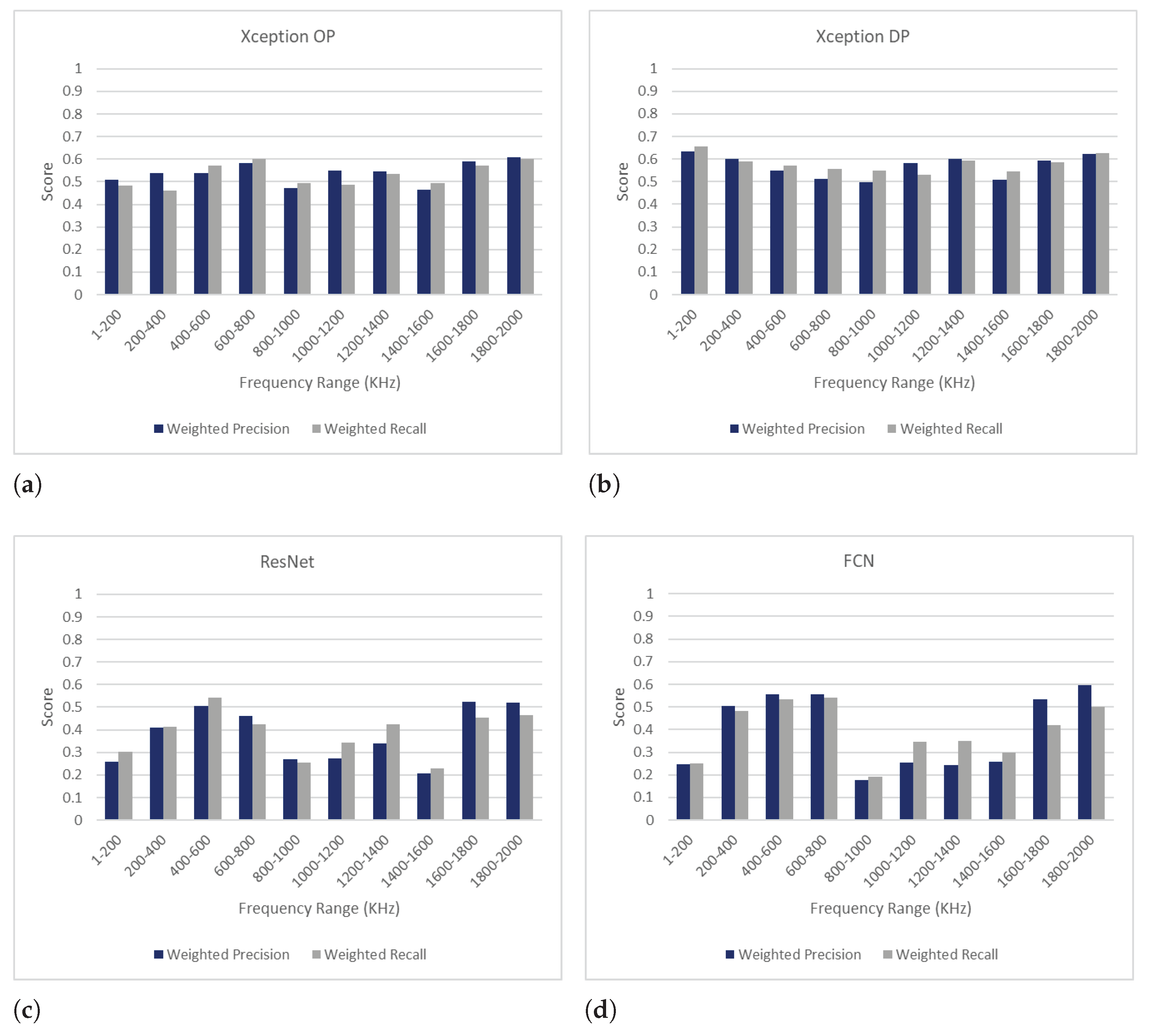
Figure 8 displays the results obtained after the application of the weighted importance transformation procedure. In this transformed scenario, Xception-DP continued to have the highest precision and recall values in the 100 kHz–200 kHz and 1.8 MHz–2 MHz regions, while the 400 kHz–600 KHz region produced the best precision and recall scores for both ResNet and FCN. The higher recall value in this region makes it a more practical option. Recall is generally more important than precision in fault classification studies. This is because while a false positive may lead to additional time spent manually double-checking FRs for faults or transformer inspection, a false negative may result in serious damage if left unchecked, compromising the security of the system [28].

There was no clear pattern suggesting whether phase or magnitude data performed better for the neural networks. However, an interesting finding emerged in the 100 kHz–200 kHz range, where the phase measurements led to significantly higher precision and recall values for all models. While the cause of this difference is unclear, it suggests that the models were better at extracting relevant features from the phase measurements in this specific frequency range than from the magnitude measurements.

It should be noted that phase measurements are typically not used in practical FRA due to the sensitivity of real-world phase measurements, which can introduce noise into the measured response [2]. This is a limitation of this study, as we only used simulated frequency responses, which do not have this issue. Therefore, further research is required into whether the performance of these neural networks on phase measurements translates to real-world frequency responses.

Additionally, several simplifications in modeling were made due to the high computational load, such as the number of ladder segments and the choice of a circuit model as opposed to a Finite Element Model. These were necessary simplifications due to available computational resources, and it is expected that higher-fidelity models could be used as digital twins to generate synthetic data specific to their physical counterparts as computational power and simulation methods continue to improve.

4. Conclusions

Deep learning holds tremendous promise as an enabler of online transformer monitoring in cases where measurable frequency bands may be limited. The findings of this study show that neural networks can achieve promising precision and recall scores even with just 200 kHz fractions of the frequency response. It is expected that as networks become larger and more advanced and as more data become available, their classification performance will continue to improve.

This study takes the first steps in exploring this research area, and proposes an approach for evaluating the performance of neural networks trained for FRA fault classification while taking into account the varying importance of each fault type. Future work should include testing on a physical transformer in order to determine the minimum data requirements for developing a training set as well as the utility of high fidelity simulation models, particularly 3D Finite element models, as digital twins for generating synthetic data to use in network training.